Solving the Multi-Depot Green Vehicle Routing Problem by a Hybrid Evolutionary Algorithm

Abstract
1. Introduction
1.1. Literature Review
1.2. Motivations and Contributions
- We first present a hybrid evolutionary algorithm by incorporating a variable neighborhood search method into the framework of an evolutionary algorithm to solve MDGVRP;
- We propose several dedicated neighborhood operators extending the previous search operators in ACO method [19] for search intensification, and the route-based crossover operator for search diversification;
- We present a distance- and quality-based replacement strategy to update the population;
- Extensive experimental results demonstrate the proposed HEA method can obtain a better trade-off in terms of the computational efficiency and solution quality in comparison with the previous ACO method in literature;
- These ideas of the proposed combined evolutionary-based framework and the variable neighborhood search suitable for solving MDGVRP are general and can be employed as a reference for other related GVRPS.
2. Problem Description and Mathematic Model
3. A Hybrid Evolutionary Algorithm for MDGVRP
3.1. The Main Framework of HEA for MDGVRP
3.2. Initial Population Phase
- Step 1: Each route of S is initialized by generating a randomly selected depot Rc as the first node and a randomly customer node as the second node.
Algorithm 1. The framework of the proposed HEA for MDGVRP. 1: Input: Problem instance , size of population
2: Output: Best found solution
3: , …,
4: for {1, …, } do
5:
6: end for
7: while the maximum running time is not met do
8: Choose two random individuals and from population P
9:
10:
11: if then
12: ,
13: end if
14:
15: end while
16: return - Step 2: As for each route, a nearest node to the last node of the current route Rc is iteratively selected and inserted into the current route Rc until the current vehicle cannot serve the remaining customers.
3.3. Variable Neighborhood Search Procedure
Neighborhood Structure
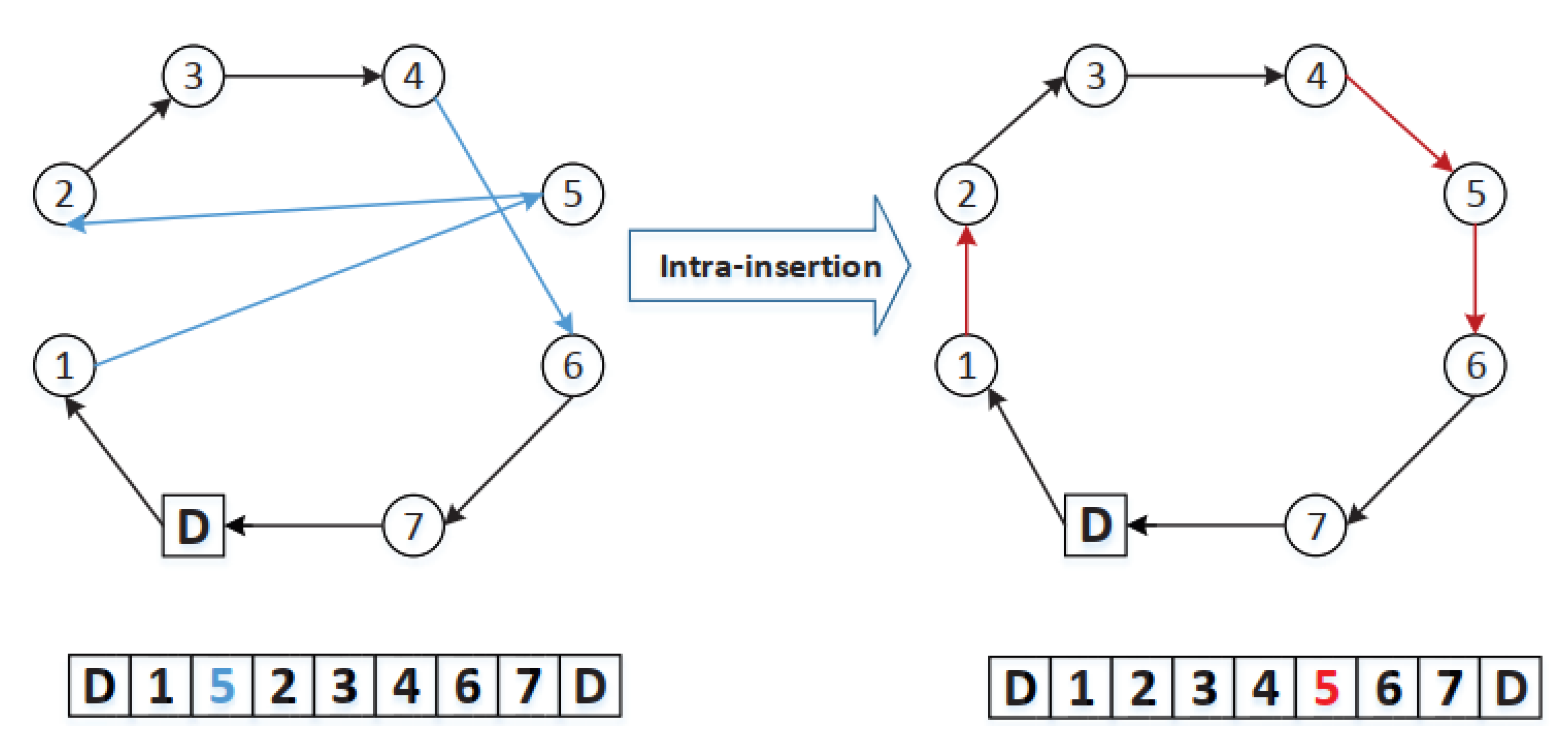
- Intra-insertion ( ): The operator chooses a customer in a route and relocates it in the current route (Figure 1);
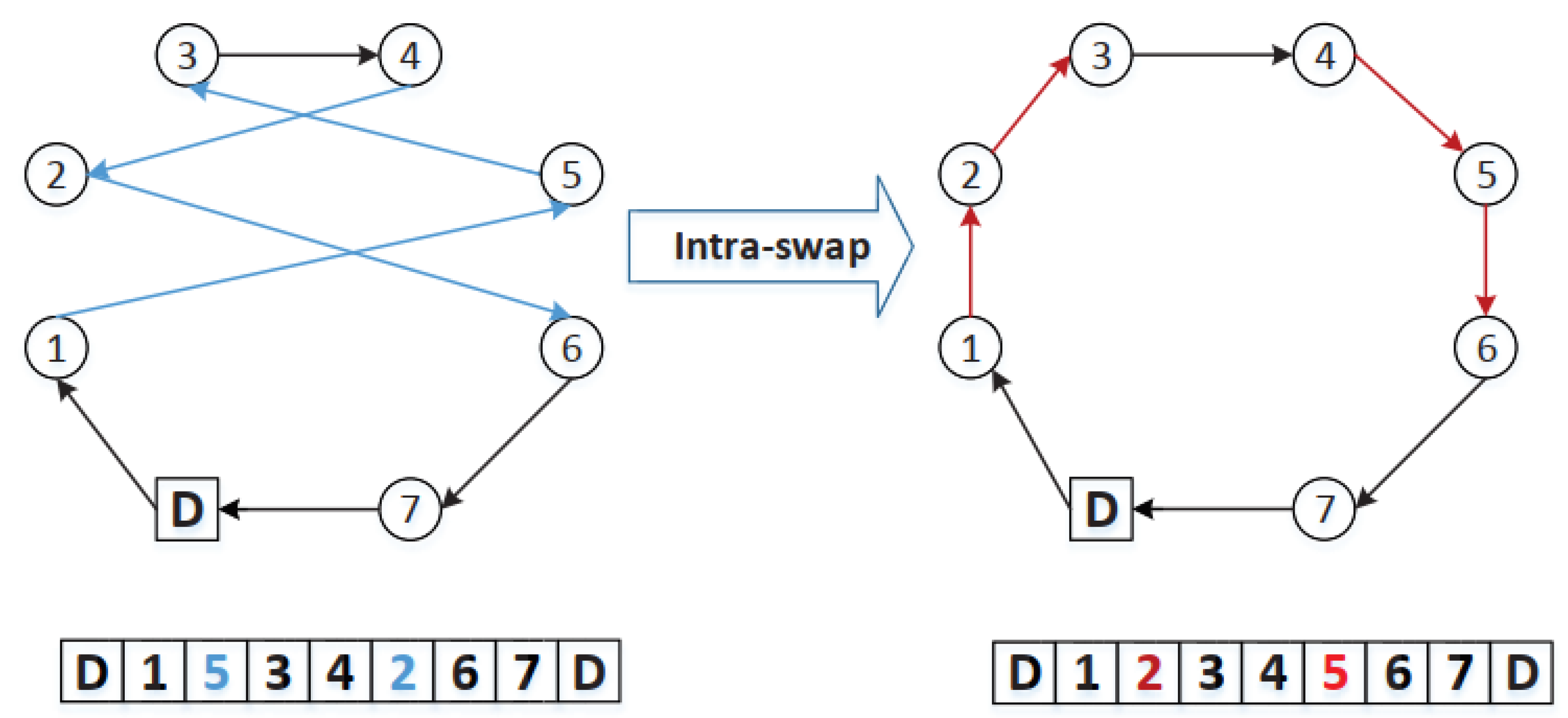
- Intra-swap (): The operator exchanges the positions of two customers in the same route (Figure 2);
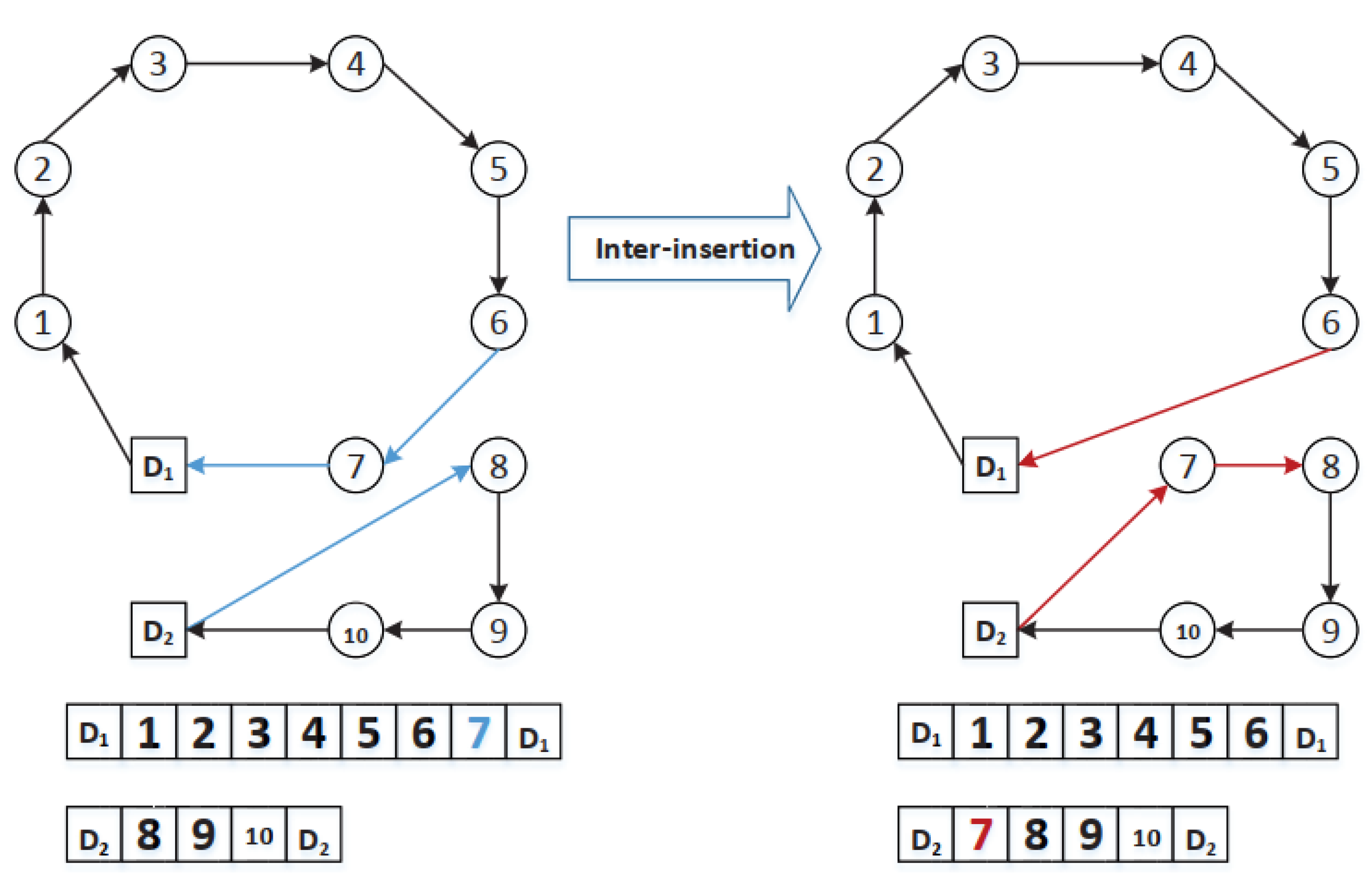
- Inter-insertion (): Unlike the intra-insertion operator (), the operator chooses a customer node from a given route and relocates it in another different route (Figure 3);
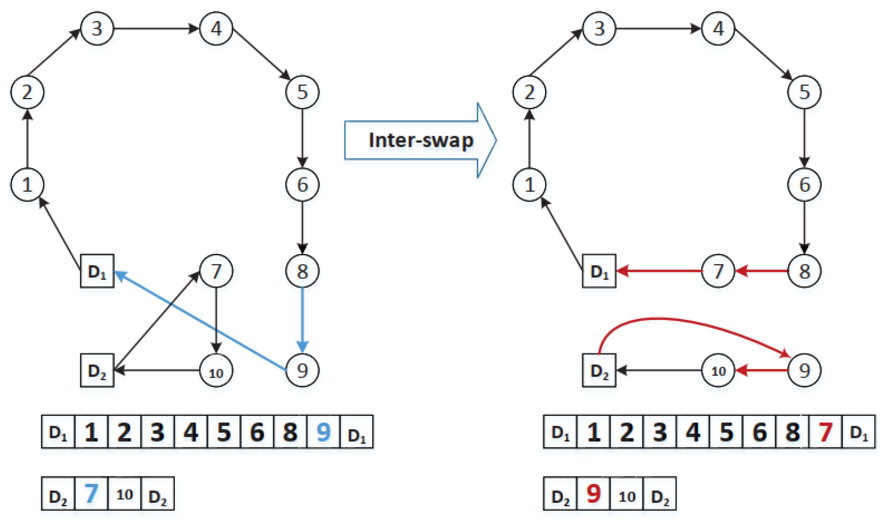
- Inter-swap (): Unlike the intra-swap operator (), the operator exchanges the positions of two customers in different routes (Figure 4);
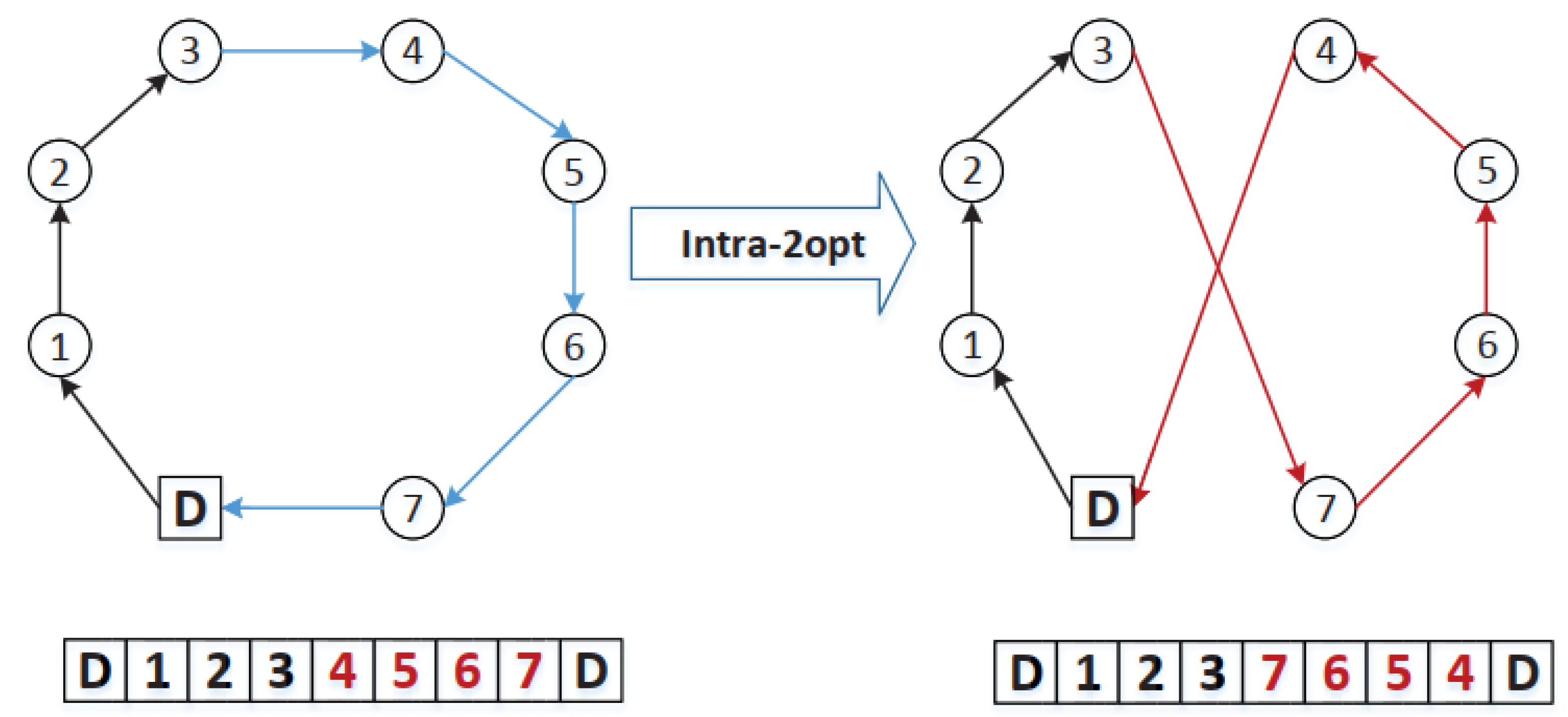
- Intra-2opt (): The operator deletes two non-adjacent edges, reverses the intermediate customer nodes in the route, and relinks the route by adding two new edges (Figure 5);
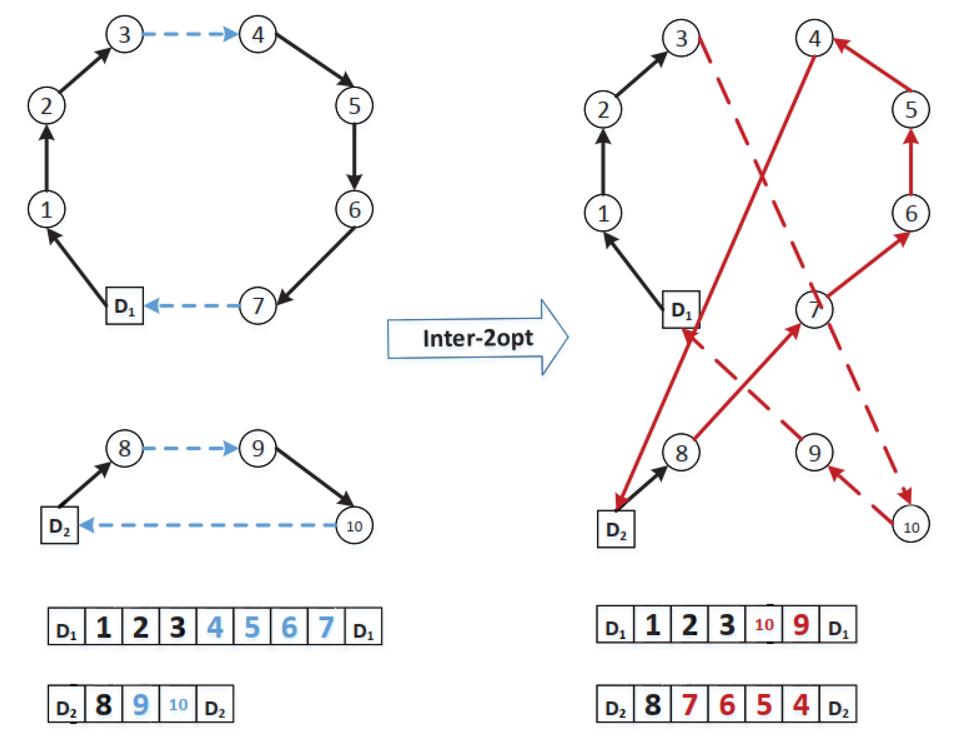
- Inter-2opt (): The operator eliminates two edges in different routes. Then, each route is cut into two parts, respectively. After that, it reverses two middle customer nodes in two routes and relinks each first part of a route with the last part of the other route to obtain two new routes (Figure 6).
| Algorithm 2. Variable neighborhood search |
| 1: Input: Initial solution ; maximum iterations without improvement 2: Output: Local optimum 3: 4: 5: 6: while Number of move operator does not exceed the maximum number (i.e., 4) of move operators (i.e., ) do 7: by using the neighborhood operator 8: if then 9: 10: 11: else 12: 13: end if 14: { , } 15: ( , ) 16: end while 17: return |
| Algorithm 3. The shaking procedure |
| 1: Input: Current solution , local optimum , the shaking strength , the interval of threshold |
| 2: Output: Perturbed solution |
| 3: |
| 4: while do |
| 5: Randomly pick a neighboring solution |
| 6: |
| 7: if then |
| 8: |
| 9: |
| 10: end if |
| 11: end while |
| 12: return |
3.4. Route-Based Crossover Operator
- Step 1: Copy one route Ri (1≤i≤K1 or K2) based on the iterated greedy strategy from two parent solutions S1 and S2 to the offspring solution. Specifically, the route with maximum value of ∆ f (Ri)/| Ri | is obtained from the parents, where ∆ f (Ri) denotes the incremental objective value after inserting the route, and | Ri | represents the number of customer nodes in route Ri.
- Step 2: Remove the customer nodes in route Ri from both two parent solutions S1 and S2.
3.5. The Distance- and Quality-Based Population Updating Mechanism
| Algorithm 4. The distance- and quality-based population updating mechanism |
| 1: Input: Population , offspring solution , distance factor parameter 2: Output: The new population after population updating strategy 3: { : ,…, } 4: the closest solution to the offspring solution according to the Hamming distance 5: the Hamming distance between the offspring solution and the closest solution 6: if and then 7: 8: else if and then 9: 10: end if 11: return |
4. Experiment Results
4.1. Benchmark Instances and Experiment Setting
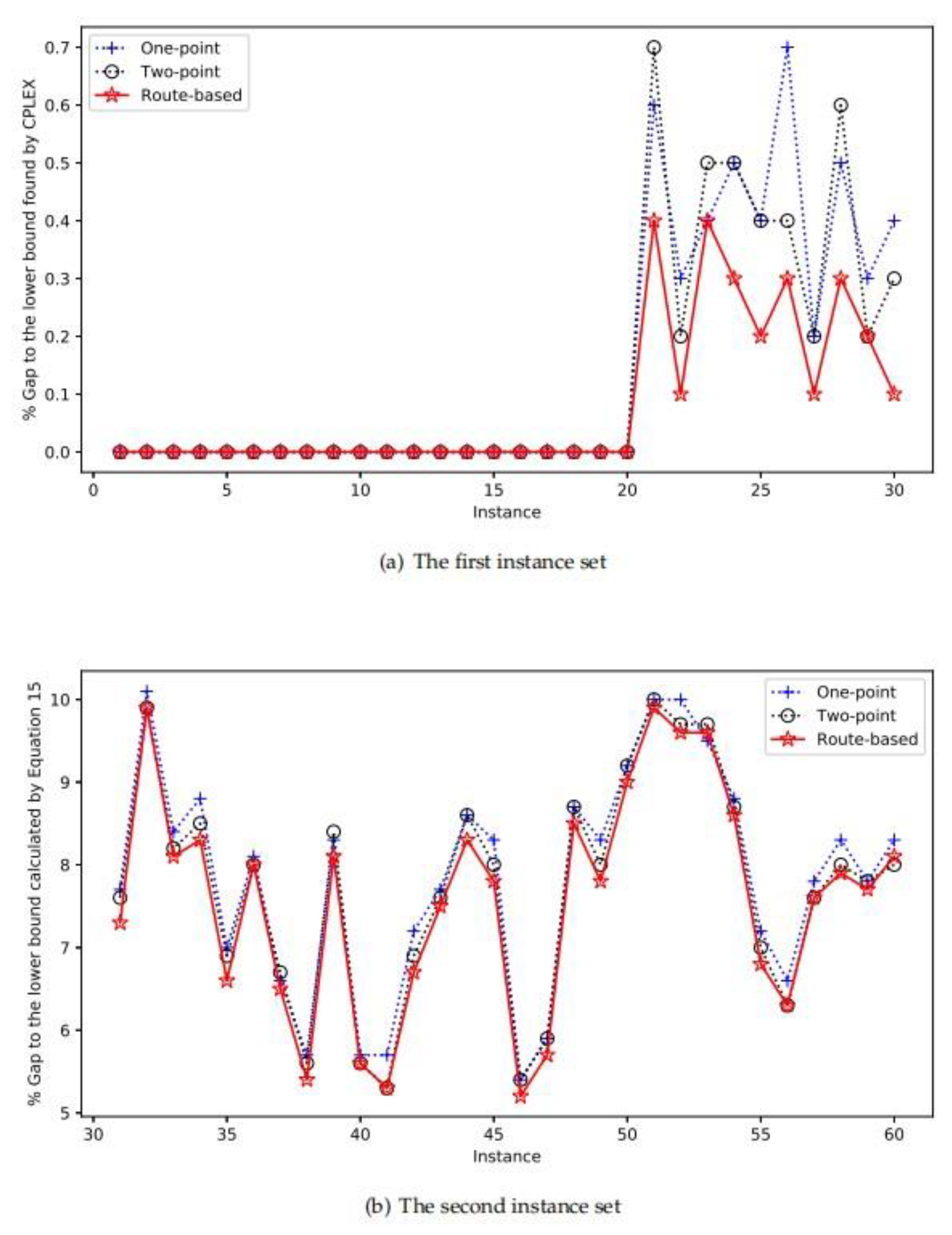
- The first instance set—The small-scale instance set with two depots and the number of customer nodes that ranged from 9 to 14 are given as follows:{The number of depots , The number of customers } = {(2,9), (2,10), (2,11), (2,12), (2,13),(2,14)};The solver CPLEX and the previous best-performing ACO procedure and the proposed HEA algorithm are used for solving the mathematical model proposed in Section 2;
- The second instance set—The large-scale instance set with the number of depots ranging from 3 to 5 and the number of customer nodes ranging from 20 to 40 are considered as follows:{The number of depots , The number of customers } = {(3,20), (3,30), (4,20), (4,30), (5,20),(5,40)};The proposed HEA algorithm and the previous best-performing ACO procedure are used for solving the mathematical model presented in Section 2.
4.2. Lower Bound
4.3. Experimental Results on the First Instance Set
4.4. Experimental Results on the Second Instance Set
5. Analysis for the Route-Based Crossover Operator
6. Discussion
7. Conclusions and Future Research
Author Contributions
Funding
Conflicts of Interest
References
- Zhou, Y.; Lee, G. A Lagrangian relaxation-based solution method for a green vehicle routing problem to minimize greenhouse gas emissions. Sustainability 2017, 9, 776. [Google Scholar] [CrossRef]
- Ubeda, S.; Arcelus, F.J.; Faulin, J. Green logistics at Eroski: A case study. Int. J. Prod. Econ. 2011, 131, 44–51. [Google Scholar] [CrossRef]
- Guo, J.X.; Tan, X.; Gu, B. The impacts of uncertainties on the carbon mitigation design: Perspective from abatement cost and emission rate. J. Clean. Prod. 2019, 232, 213–223. [Google Scholar] [CrossRef]
- Nocera, S.; Galati, O.I.; Cavallaro, F. On the uncertainty in the economic valuation of carbon emissions from transport. J. Transp. Econ. Policy 2018, 52, 68–94. [Google Scholar]
- Li, J.; Guo, H.; Zhou, Q.; Yang, B. Vehicle Routing and Scheduling Optimization of Ship Steel Distribution Center under Green Shipbuilding Mode. Sustainability 2019, 11, 4248. [Google Scholar] [CrossRef]
- Eun, J.; Song, B.D.; Lee, S.; Lim, D.E. Mathematical Investigation on the Sustainability of UAV Logistics. Sustainability 2019, 11, 5932. [Google Scholar] [CrossRef]
- Lin, C.; Choy, K.L.; Ho, G.T.; Chung, S.H.; Lam, H. Survey of green vehicle routing problem: Past and future trends. Expert Syst. Appl. 2014, 41, 1118–1138. [Google Scholar] [CrossRef]
- Braekers, K.; Ramaekers, K.; Van Nieuwenhuyse, I. The vehicle routing problem: State of the art classification and review. Comput. Ind. Eng. 2016, 99, 300–313. [Google Scholar] [CrossRef]
- Palmer, A. The Development of an Integrated Routing and Carbon Dioxide Emissions Model for Goods Vehicles. Available online: https://dspace.lib.cranfield.ac.uk/handle/1826/2547 (accessed on 7 March 2020).
- Kara, I.; Kara, B.Y.; Yetis, M.K. Energy minimizing vehicle routing problem. In International Conference on Combinatorial Optimization and Applications; Springer: Berlin/Heidelberg, Germany, 2007. [Google Scholar]
- Demir, E.; Bektas, T.; Laporte, G. A comparative analysis of several vehicle emission models for road freight transportation. Transp. Res. Part D Transp. Environ. 2011, 16, 347–357. [Google Scholar] [CrossRef]
- Kopfer, H.W.; Schönberger, J.; Kopfer, H. Reducing greenhouse gas emissions of a heterogeneous vehicle fleet. Flex. Serv. Manuf. J. 2014, 26, 221–248. [Google Scholar] [CrossRef]
- Bektas, T.; Laporte, G. The pollution-routing problem. Transp. Res. Part B Methodol. 2011, 45, 1232–1250. [Google Scholar] [CrossRef]
- Demir, E.; Bektas, T.; Laporte, G. An adaptive large neighborhood search heuristic for the pollution-routing problem. Eur. J. Oper. Res. 2012, 223, 346–359. [Google Scholar] [CrossRef]
- Demir, E.; Bektas¸, T.; Laporte, G. The bi-objective pollution-routing problem. Eur. J. Oper. Res. 2014, 232, 464–478. [Google Scholar] [CrossRef]
- Gajanand, M.; Narendran, T. Green route planning to reduce the environmental impact of distribution. Int. J. Logist. Res. Appl. 2013, 16, 410–432. [Google Scholar] [CrossRef]
- Tiwari, A.; Chang, P.C. A block recombination approach to solve green vehicle routing problem. Int. J. Prod. Econ. 2015, 164, 379–387. [Google Scholar] [CrossRef]
- Suzuki, Y. A dual-objective metaheuristic approach to solve practical pollution routing problem. Int. J. Prod. Econ. 2016, 176, 143–153. [Google Scholar] [CrossRef]
- Jabir, E.; Panicker, V.V.; Sridharan, R. Design and development of a hybrid ant colony-variable neighbourhood search algorithm for a multi-depot green vehicle routing problem. Transp. Res. Part D Transp. Environ. 2017, 57, 422–457. [Google Scholar] [CrossRef]
- Cheng, T.; Peng, B.; Lü, Z. A hybrid evolutionary algorithm to solve the job shop scheduling problem. Ann. Oper. Res. 2016, 242, 223–237. [Google Scholar] [CrossRef]
- Bansal, R.; Srivastava, K.; Srivastava, S. A hybrid evolutionary algorithm for the cutwidth minimization problem. In Proceedings of the 2012 IEEE Congress on Evolutionary Computation, Brisbane, Australia, 10–15 June 2012. [Google Scholar]
- Abdullah, S.; Burke, E.K.; McCollum, B. A hybrid evolutionary approach to the university course timetabling problem. In Proceedings of the 2007 IEEE Congress on Evolutionary Computation, Singapore, 25–28 September 2007. [Google Scholar]
- Wang, Y.; Cai, Z.; Guo, G.; Zhou, Y. Multiobjective optimization and hybrid evolutionary algorithm to solve constrained optimization problems. IEEE Trans. Syst. Man Cybern. Part B 2007, 37, 560–575. [Google Scholar] [CrossRef]
- Karabulut, K.; Tasgetiren, M.F. A variable iterated greedy algorithm for the traveling salesman problem with time windows. Inf. Sci. 2014, 279, 383–395. [Google Scholar] [CrossRef]
- Birattari, M.; Yuan, Z.; Balaprakash, P.; Stützle, T. F-Race and Iterated F-Race: An Overview. In Experimental Methods for the Analysis of Optimization Algorithms; Springer: Berlin/Heidelberg, Germany, 2010; pp. 311–336. [Google Scholar]
- Kellegöz, T.; Toklu, B.; Wilson, J. Comparing efficiencies of genetic crossover operators for one machine total weighted tardiness problem. Appl. Math. Comput. 2008, 199, 590–598. [Google Scholar] [CrossRef]
- Lu, Y.; Hao, J.K.; Wu, Q. Hybrid evolutionary search for the traveling repairman problem with profits. Inf. Sci. 2019, 502, 91–108. [Google Scholar] [CrossRef]
- Zhou, R.; Liao, Y.; Shen, W. Channel selection and fulfillment service contracts in the presence of asymmetric service information. Int. J. Prod. Econ. 2019, 107504. [Google Scholar] [CrossRef]


| Symbols | Definitions |
|---|---|
| Maximum number of customer nodes | |
| Maximum number of depots | |
| Maximum number of vehicles | |
| 1, if vehicle travels from customer node to customer node , | |
| , , | Customer index and vehicle index, respectively |
| Driving distance from customer node to customer node | |
| Fixed vehicle cost | |
| Variable vehicle cost per unit distance | |
| Volume of fuel consumption per unit vehicle weight per unit distance | |
| CO2 emissions cost per vehicle weight per unit distance | |
| Weight of every transportation product | |
| Average cost per unit weight of CO2 | |
| CO2 emission weight per liter fuel consumption | |
| Average gross weight per vehicle on each route | |
| Requirement of customer node | |
| Ratio of vehicle volume to curb weight | |
| Depot capacity | |
| Vehicle capacity |
| Parameters | Description | Candidate Values | Final Value |
|---|---|---|---|
| The number of individual solutions in the population | {5, 10, 20} | 5 | |
| The threshold of shaking strength in the shaking procedure | 3, 6, 9 | 3 | |
| Interval of threshold ratio values in the shaking procedure | (0,1) | [0.1, 0.2] | |
| Distance factor parameter in the population updating strategy | 0.05,0.1,0.2 | 0.1 |
| Instance | m | n | CPLEXLB | CPLEXUB | Gap (%) | ACO | HEA | ||||||
|---|---|---|---|---|---|---|---|---|---|---|---|---|---|
| Gap % | Gap % | ||||||||||||
| 1 | 2 | 9 | 1246.7 | 1246.7 | 0 | 1246.7 | 1246.7 | 1.1 | 0 | 1246.7 | 1246.7 | 0.1 | 0 |
| 2 | 2 | 9 | 1481.6 | 1481.6 | 0 | 1481.6 | 1481.6 | 1.3 | 0 | 1481.6 | 1481.6 | 0.9 | 0 |
| 3 | 2 | 9 | 1434.9 | 1434.9 | 0 | 1434.9 | 1434.9 | 1.5 | 0 | 1434.9 | 1434.9 | 0.2 | 0 |
| 4 | 2 | 9 | 1222.6 | 1222.6 | 0 | 1222.6 | 1222.6 | 0.9 | 0 | 1222.6 | 1222.6 | 0.6 | 0 |
| 5 | 2 | 9 | 1285.7 | 1285.7 | 0 | 1285.7 | 1285.7 | 2.3 | 0 | 1285.7 | 1285.7 | 1.1 | 0 |
| 6 | 2 | 10 | 1688.3 | 1688.3 | 0 | 1688.3 | 1688.3 | 2.8 | 0 | 1688.3 | 1688.3 | 1.1 | 0 |
| 7 | 2 | 10 | 1553.8 | 1553.8 | 0 | 1553.8 | 1553.8 | 1.7 | 0 | 1553.8 | 1553.8 | 0.8 | 0 |
| 8 | 2 | 10 | 1341.8 | 1341.8 | 0 | 1341.8 | 1341.8 | 2.1 | 0 | 1341.8 | 1341.8 | 0.9 | 0 |
| 9 | 2 | 10 | 1464.6 | 1464.6 | 0 | 1464.6 | 1464.6 | 2.8 | 0 | 1464.6 | 1464.6 | 0.5 | 0 |
| 10 | 2 | 10 | 1416.2 | 1416.2 | 0 | 1416.2 | 1416.2 | 2.2 | 0 | 1416.2 | 1416.2 | 0.9 | 0 |
| 11 | 2 | 11 | 1581.8 | 1581.8 | 0 | 1581.8 | 1581.8 | 1.2 | 0 | 1581.8 | 1581.8 | 1.2 | 0 |
| 12 | 2 | 11 | 1769.3 | 1769.3 | 0 | 1769.3 | 1769.3 | 2.9 | 0 | 1769.3 | 1769.3 | 1.9 | 0 |
| 13 | 2 | 11 | 1792.3 | 1792.3 | 0 | 1792.3 | 1792.3 | 1.5 | 0 | 1792.3 | 1792.3 | 2 | 0 |
| 14 | 2 | 11 | 1667.6 | 1667.6 | 0 | 1667.6 | 1667.6 | 1.7 | 0 | 1667.6 | 1667.6 | 0.9 | 0 |
| 15 | 2 | 11 | 1807.9 | 1807.9 | 0 | 1807.9 | 1807.9 | 1.9 | 0 | 1807.9 | 1807.9 | 0.6 | 0 |
| 16 | 2 | 12 | 1807.7 | 1846.2 | 2.1 | 1807.7 | 1892 | 1.8 | 0 | 1807.7 | 1849.4 | 0.3 | 0 |
| 17 | 2 | 12 | 1995 | 2053.7 | 2.9 | 1995 | 2013.1 | 2.1 | 0 | 1995 | 2013.3 | 0.5 | 0 |
| 18 | 2 | 12 | 1839.6 | 1940.2 | 5.5 | 1839.6 | 1861 | 1.6 | 0 | 1839.6 | 1881.6 | 1.9 | 0 |
| 19 | 2 | 12 | 1779 | 1851 | 4.1 | 1779 | 1838.8 | 2.3 | 0 | 1779 | 1780.2 | 1.7 | 0 |
| 20 | 2 | 12 | 1799.7 | 1853.3 | 2.9 | 1799.7 | 1851.1 | 3.5 | 0 | 1799.7 | 1838.7 | 1.6 | 0 |
| 21 | 2 | 13 | 1710.8 | 1765.5 | 3.2 | 1722.8 | 1765.3 | 1.3 | 0.7 | 1717.6 | 1752.2 | 1 | 0.4 |
| 22 | 2 | 13 | 1876.9 | 1928.7 | 2.8 | 1884.4 | 1976 | 3.4 | 0.4 | 1878.8 | 1931.4 | 0.7 | 0.2 |
| 23 | 2 | 13 | 1809.5 | 1916.6 | 5.9 | 1814.9 | 1850.3 | 3.9 | 0.3 | 1816.7 | 1837.9 | 1.4 | 0.5 |
| 24 | 2 | 13 | 1716 | 1802.1 | 5.0 | 1738.3 | 1804.7 | 2 | 1.3 | 1721.1 | 1782.2 | 1.4 | 0.3 |
| 25 | 2 | 13 | 1996.5 | 2097.1 | 5.0 | 2008.5 | 2080.3 | 2.1 | 0.6 | 2000.5 | 2040.5 | 1.1 | 0.2 |
| 26 | 2 | 14 | 1902.2 | 2101.9 | 10.5 | 1921.2 | 1988.7 | 2.3 | 1.2 | 1907.9 | 1943.6 | 1.3 | 0.4 |
| 27 | 2 | 14 | 1718.4 | 1908.6 | 11.1 | 1739 | 1823.3 | 3.9 | 1.2 | 1720.1 | 1764.4 | 2.5 | 0.2 |
| 28 | 2 | 14 | 1759.3 | 2035.5 | 15.8 | 1778.7 | 1794 | 3.8 | 1.1 | 1764.6 | 1807 | 1.1 | 0.4 |
| 29 | 2 | 14 | 1824.3 | 2081 | 14.1 | 1837.1 | 1917.3 | 2.9 | 0.8 | 1827.9 | 1840 | 1.5 | 0.3 |
| 30 | 2 | 14 | 1784 | 2099.4 | 17.7 | 1803.6 | 1833.6 | 2.8 | 1.2 | 1785.8 | 1812.6 | 2.2 | 0.2 |
| #Avg | 1669.1 | 1734.5 | 7.2 | 1674.2 | 1701.5 | 2.3 | 0.8 | 1670.6 | 1687.7 | 1.1 | 0.2 | ||
| #Best | 20 | 21 | 29 | ||||||||||
| Instance | m | n | LB | ACO | HEA | ||||||
|---|---|---|---|---|---|---|---|---|---|---|---|
| Gap % | Gap % | ||||||||||
| 31 | 3 | 20 | 4069.9 | 4688.5 | 4719.7 | 6.3 | 15.2 | 4367 | 4372.3 | 5.7 | 7.3 |
| 32 | 3 | 20 | 4793.2 | 5564.9 | 5638 | 6 | 16.1 | 5267.7 | 5269.7 | 4.9 | 9.9 |
| 33 | 3 | 20 | 3203.6 | 3780.2 | 3832.2 | 5.3 | 18 | 3463.1 | 3490.4 | 2.5 | 8.1 |
| 34 | 3 | 20 | 3972.6 | 4457.3 | 4532.4 | 6.9 | 12.2 | 4302.3 | 4302.7 | 5.8 | 8.3 |
| 35 | 3 | 20 | 3279.2 | 3656.3 | 3686.1 | 7 | 11.5 | 3495.6 | 3507.6 | 2.5 | 6.6 |
| 36 | 3 | 30 | 9361.6 | 11,215.2 | 11,315 | 26.1 | 19.8 | 10,110.5 | 10,139 | 9.6 | 8 |
| 37 | 3 | 30 | 7422.4 | 8172.1 | 8336.9 | 24.2 | 10.1 | 7904.9 | 7924.2 | 7.5 | 6.5 |
| 38 | 3 | 30 | 7160.4 | 8470.8 | 8622.7 | 29.2 | 18.3 | 7547.1 | 7581.8 | 10 | 5.4 |
| 39 | 3 | 30 | 7702.9 | 8935.4 | 8997 | 24.6 | 16 | 8326.8 | 8336.9 | 13.6 | 8.1 |
| 40 | 3 | 30 | 8056.4 | 9506.6 | 9703.6 | 27.6 | 18 | 8507.6 | 8514.9 | 18.7 | 5.6 |
| 41 | 4 | 20 | 3990.3 | 4417.3 | 4499.5 | 6.8 | 10.7 | 4201.8 | 4221.8 | 4.5 | 5.3 |
| 42 | 4 | 20 | 4082.4 | 4535.5 | 4642.9 | 5 | 11.1 | 4355.9 | 4382.8 | 3.1 | 6.7 |
| 43 | 4 | 20 | 6181.6 | 6972.8 | 7063.9 | 8.1 | 12.8 | 6645.2 | 6650.1 | 3.6 | 7.5 |
| 44 | 4 | 20 | 5476.2 | 6127.9 | 6156.8 | 7 | 11.9 | 5930.7 | 5979.6 | 5.1 | 8.3 |
| 45 | 4 | 20 | 6633.6 | 7641.9 | 7754.9 | 5.7 | 15.2 | 7151.3 | 7157.9 | 2 | 7.8 |
| 46 | 4 | 30 | 6239.5 | 7075.6 | 7202.8 | 44.5 | 13.4 | 6564.2 | 6597.9 | 19.2 | 5.2 |
| 47 | 4 | 30 | 6195.4 | 6969.8 | 7067.9 | 40.5 | 12.5 | 6548.5 | 6566.9 | 24.2 | 5.7 |
| 48 | 4 | 30 | 5792.3 | 6881.3 | 7026.6 | 38.9 | 18.8 | 6284.6 | 6346.7 | 23.4 | 8.5 |
| 49 | 4 | 30 | 6537.8 | 7505.4 | 7675.8 | 39.8 | 14.8 | 7047.7 | 7099.2 | 42.9 | 7.8 |
| 50 | 4 | 30 | 6761.8 | 7749 | 7821.1 | 41.6 | 14.6 | 7370.4 | 7376.5 | 36.8 | 9 |
| 51 | 5 | 20 | 5007.4 | 6003.9 | 6147.4 | 12.4 | 19.9 | 5503.1 | 5522.9 | 6.4 | 9.9 |
| 52 | 5 | 20 | 6779 | 7680.6 | 7696.3 | 9.8 | 13.3 | 7429.8 | 7479.1 | 4.2 | 9.6 |
| 53 | 5 | 20 | 3871.4 | 4363.1 | 4442.6 | 8.4 | 12.7 | 4243.1 | 4274.4 | 9.1 | 9.6 |
| 54 | 5 | 20 | 4035.1 | 4600 | 4623.7 | 9.2 | 14 | 4382.1 | 4384 | 3.5 | 8.6 |
| 55 | 5 | 20 | 3057.9 | 3458.5 | 3534.1 | 12.3 | 13.1 | 3265.8 | 3273.1 | 12.5 | 6.8 |
| 56 | 5 | 40 | 6774.6 | 7865.3 | 7931.8 | 32.1 | 16.1 | 7201.4 | 7201.5 | 27.6 | 6.3 |
| 57 | 5 | 40 | 6140 | 6809.3 | 6856.1 | 57 | 10.9 | 6606.6 | 6650.4 | 33.6 | 7.6 |
| 58 | 5 | 40 | 10,628.1 | 11,999.1 | 12,258.4 | 50 | 12.9 | 11,467.7 | 11482 | 38.7 | 7.9 |
| 59 | 5 | 40 | 9201.7 | 10,858.4 | 10,926.1 | 55.7 | 18 | 9910.2 | 9987.8 | 30.9 | 7.7 |
| 60 | 5 | 40 | 8614.4 | 10,268.4 | 10,280.1 | 40.5 | 19.2 | 9312.2 | 9356.1 | 42.7 | 8.1 |
| #Avg | 6034.1 | 6805.9 | 7033.1 | 23 | 14.7 | 6490.5 | 6514.3 | 15.1 | 7.6 | ||
| #Best | 0 | 30 | |||||||||
© 2020 by the authors. Licensee MDPI, Basel, Switzerland. This article is an open access article distributed under the terms and conditions of the Creative Commons Attribution (CC BY) license (http://creativecommons.org/licenses/by/4.0/).
Share and Cite
Peng, B.; Wu, L.; Yi, Y.; Chen, X. Solving the Multi-Depot Green Vehicle Routing Problem by a Hybrid Evolutionary Algorithm. Sustainability 2020, 12, 2127. https://doi.org/10.3390/su12052127
Peng B, Wu L, Yi Y, Chen X. Solving the Multi-Depot Green Vehicle Routing Problem by a Hybrid Evolutionary Algorithm. Sustainability. 2020; 12(5):2127. https://doi.org/10.3390/su12052127
Chicago/Turabian StylePeng, Bo, Lifan Wu, Yuxin Yi, and Xiding Chen. 2020. "Solving the Multi-Depot Green Vehicle Routing Problem by a Hybrid Evolutionary Algorithm" Sustainability 12, no. 5: 2127. https://doi.org/10.3390/su12052127
APA StylePeng, B., Wu, L., Yi, Y., & Chen, X. (2020). Solving the Multi-Depot Green Vehicle Routing Problem by a Hybrid Evolutionary Algorithm. Sustainability, 12(5), 2127. https://doi.org/10.3390/su12052127