Risk Management Opportunities between Socially Responsible Investments and Selected Commodities


Abstract
1. Introduction
2. Literature Review
3. Materials and Methods
- -
- normal—multivariate Student’s t,
- -
- Student’s t—multivariate normal,
- -
- Student’s t—multivariate Student’s t,
- -
- normal—multivariate Laplace,
- -
- Student’s t—multivariate Laplace.
4. Results
4.1. Dataset
- -
- 2 ESG indices for the global market—Stoxx Global ESG Impact, Dow Jones Sustainability World Index;
- -
- 3 ESG indices for the European market—Stoxx Europe Industry Neutral, Stoxx Europe ESG Leaders Select 30, Dow Jones Sustainability Europe;
- -
- 2 ESG indices for the US market—Dow Jones Sustainability US Composite Index, S&P 500 ESG Index;
- -
- 2 non-ESG indices—Euro Stoxx Select Dividend 30, SP 500;
- -
- 3 commodity indices (Dow Jones Commodity Index Industrial Metals, Dow Jones Precious Metals Index, Dow Jones Commodity Grains Index).
- -
- Stationary;
- -
- For most indices, autocorrelation exists in returns and in squared returns—only for commodity indices is the null hypothesis not rejected (there is no autocorrelation in returns and in squared returns present);
- -
- For most indices, the ARCH effect is present—only for metals is the null hypothesis not rejected (there is no ARCH effect).
4.2. Volatility and Dynamic Conditional Correlation
- January 2010–July 2011 (economic growth);
- August 2011–December 2015 (a collapse in the metals market);
- January 2016–December 2017 (economic growth in metals and financial markets).
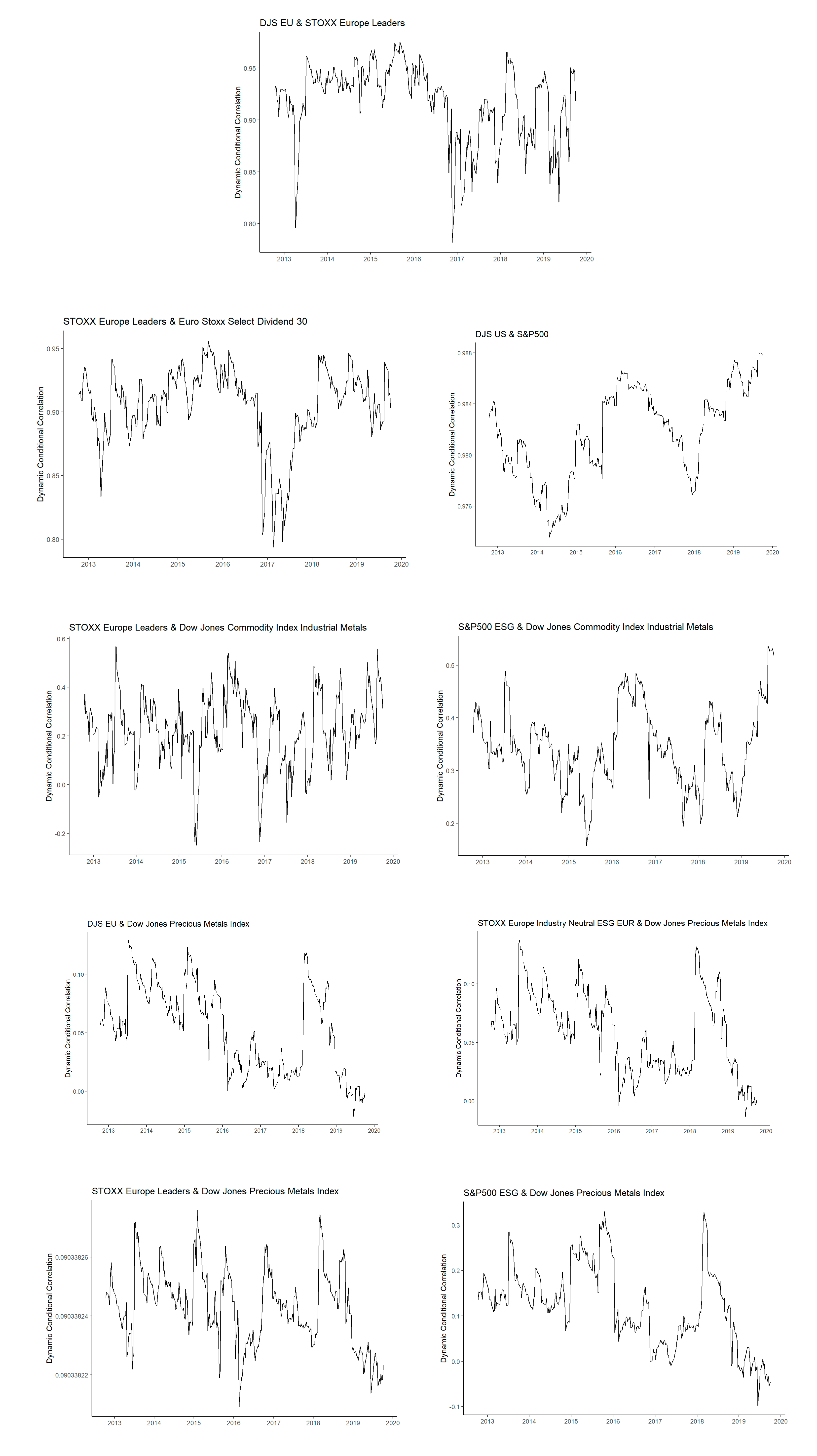
- For the ESG–ESG relationship, one pair of indices (out of 5) showed statistically significant high conditional correlation. In the last year, this correlation has been weakening, but still remains close to 1.
- In the case of the ESG–non-ESG relationship, two pairs of indices (out of 5) show statistically significant high conditional correlation (close to 1). For the European market, we observed two periods where the correlation was weakening considerably, mainly in the years 2013—a drop to 0.4 (the problem of the banking sector in the EU)—and in 2016/2017, a drop by −0.2 (the start of economic growth). For the American market, there were few periods where correlation was weakening but still remained high. The level of correlation is higher for the American market comparing to the European one.
- Eight pairs of indices (out of a total of 21) for the ESG–commodities relationship showed statistically significant low and medium (lower than 0.5) conditional correlation.
- The ESG—precious metals relationship is characterized by low correlation (less than 0.15). Four pairs of indices (out of seven) showed a growth in correlation in 2013–2015 (the beginning and the end of the downturn period on the metals market) and also in 2018, but of not more than around 0.1. The evolution of conditional correlations for the European market as represented by three indices looks very similar. For the American market, the level of correlation is higher—even more than 0.3.
- For the ESG—industrial metals relationship, two pairs of indices (out of seven) behave similarly for the European and American markets, but there are substantial differences. For the European indices, we observed three periods where the correlation is higher than 0.5, mainly in 2013 (the collapse period of the metals market), 2016 (the economic growth period in the metals and financial markets), and 2019, and also lower than 0 (−0.5) in 2015 and 2016–2017 (two drops). For the American indices, we observed one period where the correlation is higher than 0.5, mainly in 2019. Moreover, the volatility is higher in the case of European market.
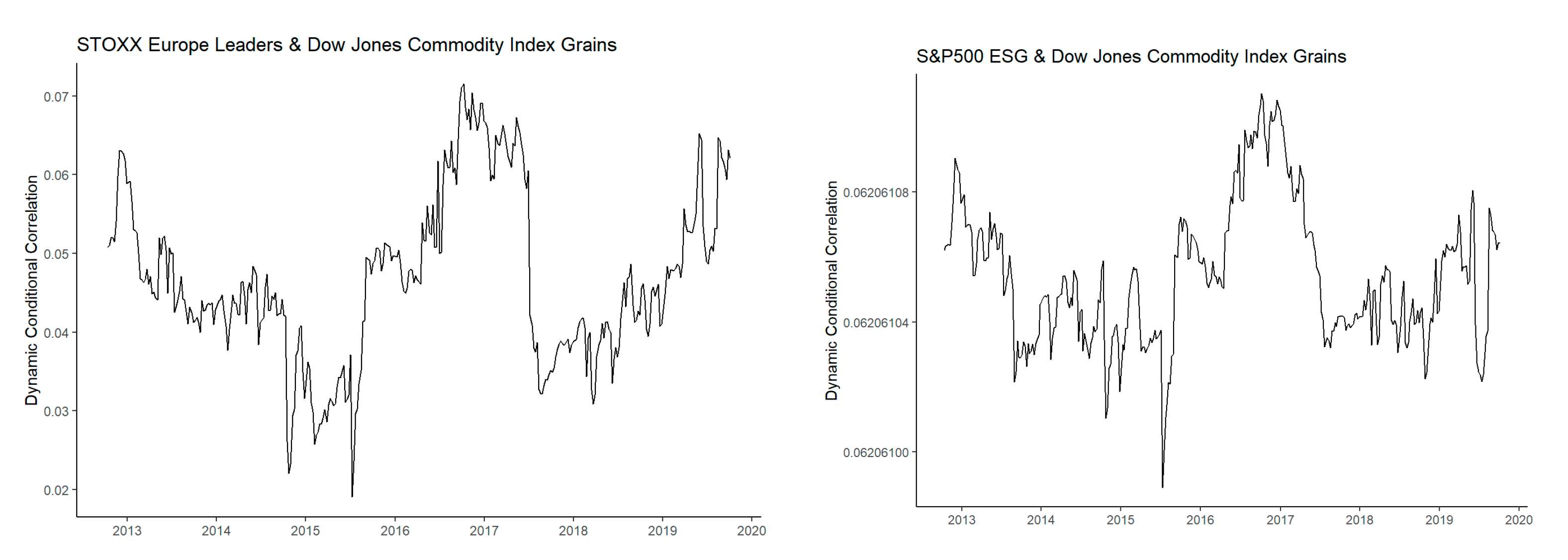
- The ESG—grains relationship is weaker compared to two earlier described relationships, around 0.06. Two pairs of indices out of seven behave similarly for the European and American markets, but there are substantial differences in some subperiods. For both markets, we observed one period where the correlation is higher than 0.06, mainly in 2013 (one pick) and 2016–2017 (the economic growth period on metals market and financial markets), and also lower than 0.02 in 2015 (the collapse period on metals market). Moreover, volatility is considerably lower in the case of the American market.
5. Discussion
- -
- -
- -
6. Conclusions
Author Contributions
Funding
Conflicts of Interest
Appendix A

| Index | Ticker | Number of Constituents | Criteria | Sectors | Weights | First Value | |
|---|---|---|---|---|---|---|---|
| Stoxx Global ESG Impact | SXEIMGGR | 889 | Stoxx Global 1800 without excluded sectors and high ESG score in every sector | 1. Technology 2. Banks 3. Health Care | Free-float | Sep 17, 2010 | |
| Stoxx Europe Industry Neutral | SXESEN | 471 | Stoxx Global 1800 without excluded sectors, and Sustainability score above 50 | 1. Health Care 2. Industrial Goods and Services 3. Banks | Free-float | Sep 24, 2012 | |
| Stoxx Europe ESG Leaders Select 30 | SEESGSEG | 30 | Dividend-paying, high liquidity European companies included in Global ESG Index | 1. Utilities 2. Insurance 3. Telecommunications | Inverted volatility | Jun 21, 2004 | |
| Euro Stoxx Select Dividend 30 | SD3E | 30 | High-dividend-yielding companies across the 11 Eurozone countries | Insurance Banks | Annual net dividend yield | Dec 30, 1998 | |
| Global Sustainability Leader Index | GSLI | Top 100 representative group of companies | Companies selected on the basis of their ESG performance. excluding companies involved in tobacco | x | Free Float Market Cap | Oct 1st, 2012 | |
| Dow Jones Sustainability US Composite Index | AASGI | 126 | The top 20% of 600 largest in the Dow Jones Sustainability North America Index | x | Modified market cap | Dec 31, 1998 | |
| Dow Jones Sustainability Europe | DJSEUR | 126 | The top 20% of the largest 600 European companies in the S&P Global BMI based on long-term economic, environmental and social criteria | Health care Consumer staples Financials | float-adjusted market capitalization | Aug 4, 2010 | |
| S&P 500 ESG Index | SPXESUP | 315 | S&P 500 companies without excluded sectors, without low 5% in terms of UNCG score and without 25% of ESG score | 1. Information technology 2. Health Care 3. Financials | Float-adjusted market cap | April 30, 2010 | |
| Dow Jones Commodity Index Industrial Metals | DJCIIM | x | Industrial Metals based through futures contracts | x | Capped | July 1, 2014 | |
| Dow Jones Precious Metals Index | DJGSP | 30 | US companies engaged in the exploration and production of gold, silver and platinum-group metals | x | Float-adjusted market cap | December 30, 2000 | |
| Dow Jones Commodity Index Grains | DJCIGR | - | Grains sector through futures contracts | x | Capped | Jan 17, 2006 | |
| Index | ADF Stat and (p-Value) | Ljung–Box r Stat and (p-Value) | Ljung–Box r2 Stat and (p-Value) | ARCH-LM Test and (p-Value) |
|---|---|---|---|---|
| DJS Europe | −7.564 (0.01) | 6.979 (0.0082) | 14.32 (0.0002) | 45.09 (0) |
| DJS US | −7.495 (0.01) | 8.532 (0.0035) | 7.559 (0.006) | 27.44 (0.0067) |
| DJ Commodity Index Grains | −7.423 (0.01) | 0.1851 (0.6671) | 1.141 (0.2855) | 26.47 (0.0092) |
| DJ Commodity Index Industrial Metals | −6.892 (0.01) | 1.114 (0.2911) | 2.011 (0.1562) | 18.29 (0.1071) |
| DJ Commodity Index Precious Metals | −6.629 (0.01) | 0 (0.9975) | 1.28 (0.258) | 30.98 (0.002) |
| GSLI | −7.74 (0.01) | 6.436 (0.0112) | 3.468 (0.0626) | 17.88 (0.1193 |
| S&P500 | −7.738 (0.01) | 6.78 8 (0.0092) | 7.72 (0.0055) | 25.3 (0.0135 |
| S&P500 ESG | −7.605 (0.01) | 7.7 (0.0055) | 7.578 (0.0059) | 24.52 (0.0173 |
| Stoxx Europe IN | −7.7 (0.01) | 6.415 (0.0113) | 16.05 (0.0001) | 42.16 (0) |
| Stoxx Europe ESG Leaders | −8.135 (0.01) | −4.619 (0.0316) | 18.97 (0) | 38.41 (0.0001) |
| Euro Stoxx Select Dividend 30 | −8.297 (0.0)1 | 7.859 (0.0051) | 18.01 (0) | 37.02 (0.0002) |
| Stoxx Global ESG Impact | −7.828 (0.01) | 6.796 (0.0091) | 5.492 (0.0191) | 22.62 (0.0311) |
| JB Test Stat | JB Test p-value | JB Test Stat (Squared Residuals) | JB Test p-VALUE (Squared Residuals) | |
|---|---|---|---|---|
| DJS Europe and Stoxx Europe ESG Leaders | ||||
| DJS Europe | 8.715 | 0.0175 | 1212 | 0 |
| Stoxx Europe ESG Leaders | 25.14 | 0.002 | 14,072 | 0 |
| Stoxx Europe ESG Leaders and Euro Stoxx Select Dividend 30 | ||||
| Stoxx Europe ESG Leaders | 44.22 | 0 | 26,708 | 0 |
| Euro Stoxx Select Dividend 30 | 0.4084 | 0.81 | 1399 | 0 |
| DJS US and S&P 500 | ||||
| DJS US | 3.611 | 0.142 | 2386 | 0 |
| S&P 500 | 27.83 | 0.0005 | 5921 | 0 |
| Stoxx Europe ESG Leaders and DJ Commodity Index Industrial Metals | ||||
| Stoxx Europe ESG Leaders | 45 | 0 | 6131 | 0 |
| DJ Commodity Index Industrial Metals | 4.912 | 0.0805 | 6465 | 0 |
| S&P500 ESG and DJ Commodity Index Industrial Metals | ||||
| S&P500 ESG | 157.6 | 0 | 38,957 | 0 |
| DJ Commodity Index Industrial Metals | 4.316 | 0.0975 | 4121 | 0 |
| DJS Europe and DJ Commodity Index Precious Metals | ||||
| DJS Europe | 40.66 | 0 | 3628 | 0 |
| DJ Commodity Index Precious Metals | 38.42 | 0 | 8879 | 0 |
| Stoxx Europe Industry Neutral and DJ Index Precious Metals | ||||
| Stoxx Europe Industry Neutral | 41.13 | 0.0005 | 5657 | 0 |
| DJ Index Precious Metals | 38.26 | 0 | 8919 | 0 |
| Stoxx Europe Leaders and DJ Index Precious Metals | ||||
| Stoxx Europe Leaders | 37.59 | 0 | 7340 | 0 |
| DJ Index Precious Metals | 29.23 | 0.0005 | 9142 | 0 |
| S&P500 ESG and DJ Index Precious Metals | ||||
| S&P500 ESG | 184.1 | 0 | 23,099 | 0 |
| DJ Index Precious Metals | 37.51 | 0.0005 | 8839 | 0 |
| Stoxx Europe Leaders and DJ Commodity Index Grains | ||||
| Stoxx Europe Leaders | 48.51 | 0 | 6892 | 0 |
| DJ Commodity Index Grains | 16.53 | 0.0025 | 9747 | 0 |
| S&P500 ESG and DJ Commodity Index Grains | ||||
| S&P500 ESG | 184.4 | 0 | 30,952 | 0 |
| DJ Commodity Index Grains | 17.1 | 0.002 | 9933 | 0 |
| JB Test Stat | JB Test p-value | JB test Stat (Squared Residuals) | JB Test p-value (Squared Residuals) | |
|---|---|---|---|---|
| DJS Europe and Stoxx Europe ESG Leaders | ||||
| DJS Europe | 8.752 | 0.018 | 1216 | 0 |
| Stoxx Europe ESG Leaders | 25.16 | 0 | 14,128 | 0 |
| Stoxx Europe ESG Leaders and Euro Stoxx Select Dividend 30 | ||||
| Stoxx Europe ESG Leaders | 44.26 | 0.001 | 26,716 | 0 |
| Euro Stoxx Select Dividend 30 | 0.4151 | 0.7995 | 1402 | 0 |
| DJS US and S&P 500 | ||||
| DJS US | 3.643 | 0.148 | 2396 | 0 |
| S&P 500 | 27.99 | 0.0005 | 5954 | 0 |
| Stoxx Europe ESG Leaders and DJ Commodity Index Industrial Metals | ||||
| Stoxx Europe ESG Leaders | 44.89 | 0.0005 | 6135 | 0 |
| DJ Commodity Index Industrial Metals | 4.924 | 0.072 | 6463 | 0 |
| S&P500 ESG and DJ Commodity Index Industrial Metals | ||||
| S&P500 ESG | 157.8 | 0 | 38975 | 0 |
| DJ Commodity Index Industrial Metals | 4.321 | 0.0905 | 4123 | 0 |
| DJS Europe and DJ Commodity Index Precious Metals | ||||
| DJS Europe | 40.7 | 0 | 3637 | 0 |
| DJ Commodity Index Precious Metals | 38.41 | 0 | 8865 | 0 |
| Stoxx Europe Industry Neutral and DJ Index Precious Metals | ||||
| Stoxx Europe Industry Neutral | 41.15 | 0 | 5660 | 0 |
| DJ Index Precious Metals | 38.25 | 0 | 8906 | 0 |
| Stoxx Europe Leaders and DJ Index Precious Metals | ||||
| Stoxx Europe Leaders | 74.35 | 0 | 13,870 | 0 |
| DJ Index Precious Metals | 29.23 | 0.0005 | 2673 | 0 |
| S&P500 ESG and DJ Index Precious Metals | ||||
| S&P500 ESG | 184.1 | 0 | 23,089 | 0 |
| DJ Index Precious Metals | 37.5 | 0.0005 | 8832 | 0 |
| Stoxx Europe Leaders and DJ Commodity Index Grains | ||||
| Stoxx Europe Leaders | 48.5 | 0 | 6891 | 0 |
| DJ Commodity Index Grains | 16.52 | 0.0055 | 9748 | 0 |
| S&P500 ESG and DJ Commodity Index Grains | ||||
| S&P500 ESG | 184.4 | 0 | 30,952 | 0 |
| DJ Commodity Index Grains | 17.1 | 0.0035 | 9933 | 0 |
| JB Test Stat | JB Test p-Value | JB Test Stat (Squared Residuals) | JB Test p-Value (Squared Residuals) | |
|---|---|---|---|---|
| DJS Europe and Stoxx Europe ESG Leaders | ||||
| DJS Europe | 8.607 | 0.019 | 1192 | 0 |
| Stoxx Europe ESG Leaders | 24.24 | 0 | 14,448 | 0 |
| Stoxx Europe ESG Leaders and Euro Stoxx Select Dividend 30 | ||||
| Stoxx Europe ESG Leaders | 43.69 | 0 | 27,212 | 0 |
| Euro Stoxx Select Dividend 30 | 0.4202 | 0.8155 | 1437 | 0 |
| DJS US and S&P 500 | ||||
| DJS US | 2.998 | 0.1885 | 2058 | 0 |
| S&P 500 | 25.56 | 0 | 5475 | 0 |
| Stoxx Europe ESG Leaders and DJ Commodity Index Industrial Metals | ||||
| Stoxx Europe ESG Leaders | 44.99 | 0 | 6143 | 0 |
| DJ Commodity Index Industrial Metals | 5.004 | 0.081 | 6429 | 0 |
| S&P500 ESG and DJ Commodity Index Industrial Metals | ||||
| S&P500 ESG | 157.8 | 0 | 38,991 | 0 |
| DJ Commodity Index Industrial Metals | 4.39 | 0.097 | 4160 | 0 |
| DJS Europe and DJ Commodity Index Precious Metals | ||||
| DJS Europe | 41.47 | 0 | 3692 | 0 |
| DJ Commodity Index Precious Metals | 38.32 | 0 | 9018 | 0 |
| Stoxx Europe Industry Neutral and DJ Index Precious Metals | ||||
| Stoxx Europe Industry Neutral | 41.75 | 0 | 5617 | 0 |
| DJ Index Precious Metals | 38.13 | 0.0005 | 9050 | 0 |
| Stoxx Europe Leaders and DJ Index Precious Metals | ||||
| Stoxx Europe Leaders | 46.19 | 0 | 7400 | 0 |
| DJ Index Precious Metals | 37.42 | 0.0005 | 9218 | 0 |
| S&P500 ESG and DJ Index Precious Metals | ||||
| S&P500 ESG | 191.1 | 0 | 22,555 | 0 |
| DJ Index Precious Metals | 37.36 | 0 | 8814 | 0 |
| S&P500 ESG and DJ Commodity Index Grains | ||||
| S&P500 ESG | 184.5 | 0 | 30,978 | 0 |
| DJ Commodity Index Grains | 17.08 | 0.0035 | 9927 | 0 |
Appendix B
| Europe—ESG Indices | ||
| DJS Europe | Stoxx Europe ESG Leaders | Insignificant |
| DJS Europe | Stoxx Europe IN | Significant |
| Stoxx Europe IN | Stoxx Europe ESG Leaders | Insignificant |
| ESG indices and non-ESG indices | ||
| DJS Europe | Euro Stoxx Select Dividend 30 | Insignificant |
| Stoxx Europe IN | Euro Stoxx Select Dividend 30 | Insignificant |
| Stoxx Europe ESG Leaders | Euro Stoxx Select Dividend 30 | Significant |
| ESG Indices and Commodity indices | ||
| DJS Europe | Dow Jones Commodity Index Industrial Metals | Insignificant |
| DJS Europe | Dow Jones Commodity Index Precious Metals | Significant |
| DJS Europe | Dow Jones Commodity Index Grains | Insignificant |
| Stoxx Europe IN | Dow Jones Commodity Index Industrial Metals | Insignificant |
| Stoxx Europe IN | Dow Jones Commodity Index Precious Metals | Significant at 0.1 |
| Stoxx Europe IN | Dow Jones Commodity Index Grains | Insignificant |
| Stoxx Europe ESG Leaders | Dow Jones Commodity Industrial Index Metals | Significant |
| Stoxx Europe ESG Leaders | Dow Jones Commodity Index Precious Metals | Significant |
| Stoxx Europe ESG Leaders | Dow Jones Commodity Index Grains | Significant |
| USA—ESG indices | ||
| DJS US | S&P 500 ESG | Insignificant |
| ESG indices and non-ESG indices | ||
| DJS US | S&P 500 | Significant |
| S&P 500 ESG | S&P 500 | Insignificant |
| ESG Indices and Commodity indices | ||
| DJS US | Dow Jones Commodity Index Industrial Metals | Insignificant |
| DJS US | Dow Jones Commodity Index Precious Metals | Insignificant |
| DJS US | Dow Jones Commodity Index Grains | Insignificant |
| SP 500 ESG | Dow Jones Commodity Index Industrial Metals | Significant |
| SP 500 ESG | Dow Jones Commodity Index Precious Metals | Significant at 0.06 |
| SP 500 ESG | Dow Jones Commodity Index Grains | Significant |
| Global—ESG indices | ||
| GSLI | Stoxx Global ESG Impact | Insignificant |
| ESG Indices and Commodity indices | ||
| Stoxx Global ESG Impact | Dow Jones Commodity Index Industrial Metals | Insignificant |
| Stoxx Global ESG Impact | Dow Jones Commodity Index Precious Metals | Insignificant |
| Stoxx Global ESG Impact | Dow Jones Commodity Index Grains | Insignificant |
| GSLI | Dow Jones Commodity Index Industrial Metals | Insignificant |
| GSLI | Dow Jones Commodity Index Precious Metals | Insignificant |
| GSLI | Dow Jones Commodity Index Grains | Insignificant |
References
- Report on US Sustainable Responsible and Impact Investing Trends 2018, US SIF Foundation. Available online: https://www.ussif.org/files/Trends/Trends%202018%20executive%20summary%20FINAL.pdf (accessed on 3 November 2019).
- Schueth, S. Socially Responsible Investing in the United States. J. Bus. Ethics 2003, 43, 189–194. [Google Scholar] [CrossRef]
- Kempf, A.; Osthoff, P. The Effect of Socially Responsible Investing on Portfolio Performance. Centre for Financial Research (CFR), Working Paper, No. 06-10, University of Cologne. 2007. Available online: http://hdl.handle.net/10419/57725 (accessed on 3 November 2019).
- Mackey, A.; Mackey, T.B.; Barney, J.B. Corporate Social Responsibility and Firm Performance: Investor Preferences and Corporate Strategies. Acad. Manag. Rev. 2007, 32, 817–835. [Google Scholar] [CrossRef]
- Auer, B.R.; Schuhmacher, F. Do socially (ir)responsible investments pay? New evidence from international ESG data. Q. Rev. Econ. Financ. 2016, 59, 51–62. [Google Scholar] [CrossRef]
- Fritz, T.M.; von Schnurbein, G. Beyond Socially Responsible Investing: Effects of Mission-Driven Portfolio Selection. Sustainability 2019, 11, 6812. [Google Scholar] [CrossRef]
- Biasin, M.; Cerqueti, R.; Giacomini, E.; Marinelli, N.; Quaranta, A.G.; Riccetti, L. Macro Asset Allocation with Social Impact Investments. Sustainability 2019, 11, 3140. [Google Scholar] [CrossRef]
- Markowitz, H. Portfolio Selection. J. Financ. 1952, 7, 77–91. [Google Scholar]
- Engle, R.F. Autoregressive Conditional Heteroscedasticity with Estimates of the Variance of United Kingdom Inflation. Econometrica 1982, 50, 987–1007. [Google Scholar] [CrossRef]
- Bollerslev, T. Generalized autoregressive conditional heteroscedasticity. J. Econom. 1986, 31, 307–327. [Google Scholar] [CrossRef]
- Engle, R.F. Dynamic conditional correlation: A simple class of multivariate generalized autoregressive conditional heteroskedasticity models. J. Bus. Econ. Stat. 2002, 20, 339–350. [Google Scholar] [CrossRef]
- Ibbotson Associates. Strategic Asset Allocation and Commodities; Ibbotson Associates: Chicago, IL, USA, 2006. [Google Scholar]
- Global Sustainable Investment Alliance. Global Sustainable Investment Review; Global Sustainable Investment Alliance: Washington, DC, USA, 2014. [Google Scholar]
- Webley, P.; Lewis, A.; Mackenzie, C. Commitment among Ethical Investors: An Experimental Approach. J. Econ. Psychol. 2001, 22, 27–42. [Google Scholar] [CrossRef]
- Ariely, D.; Bracha, A.; Meier, S. Doing Good or Doing Well? Image Motivation and Monetary Incentives in Behaving Prosocially. Am. Econ. Rev. 2009, 99, 544–555. [Google Scholar] [CrossRef]
- Ortas, E.; Burritt, R.L.; Moneva, J.M. Socially responsible investment and cleaner production in the Asia Pacific: Does it pay to be good? J. Clean. Prod. 2013, 52, 272–280. [Google Scholar] [CrossRef]
- Goyal, M.M.; Aggarwal, K. ESG Index is Good for Socially Responsible Investor in India. Asian J. Multidiscip. Stud. 2014, 2, 92–96. [Google Scholar]
- Sudha, S. Risk-Return and Volatility Analysis of Sustainability Index in India. Environ. Dev. Sustain. 2015, 17, 1329–1342. [Google Scholar] [CrossRef]
- Fatemi, A.; Glaum, M.; Kaiser, S. ESG Performance and Firm Value: The Moderating Role of Disclosure. Glob. Financ. J. 2017, 38, 45–64. [Google Scholar] [CrossRef]
- Beal, D.J.; Goyen, M.; Phillips, P. Why Do We Invest Ethically? J. Invest. 2005, 14, 66–77. [Google Scholar] [CrossRef]
- Bello, Z. Socially responsible investing and portfolio diversification. J. Financ. Res. 2005, 28, 41–57. [Google Scholar] [CrossRef]
- Benson, K.L.; Brailsford, T.J.; Humphrey, J.E. Do socially responsible fund managers really invest differently? J. Bus. Ethics 2006, 65, 337–357. [Google Scholar] [CrossRef]
- Cortez, M.C.; Silva, F.; Areal, N. Socially responsible investing in the global market: The performance of US and European funds. Int. J. Financ. Econ. 2012, 17, 254–271. [Google Scholar] [CrossRef]
- Bauer, R.; Otten, R.; Rad, A. Ethical investing in Australia: Is there a financial penalty? Pac. Basin Financ. J. 2006, 14, 33–48. [Google Scholar] [CrossRef]
- Statman, M. Socially responsible indexes: Composition, performance, and tracking error. J. Portf. Manag. 2006, 32, 100–109. [Google Scholar] [CrossRef]
- Skiadopoulos, G. Advances in the commodity futures literature: A review. J. Deriv. 2013, 20, 85–96. [Google Scholar] [CrossRef]
- Cheung, C.S.; Miu, P. Diversification benefits of commodity futures. J. Int. Financ. Mark. Inst. Money 2010, 20, 451–474. [Google Scholar] [CrossRef]
- Belousova, J.; Dorfleitner, G. On the diversification benefits of commodities from the perspective of euro investors. J. Bank. Financ. 2012, 36, 2455–2472. [Google Scholar] [CrossRef]
- Daskalaki, C.; Skiadopoulos, G.; Topaloglou, N. Diversification benefits of commodities: A stochastic dominance efficiency approach. J. Empir. Financ. 2017, 44, 250–269. [Google Scholar] [CrossRef]
- Cao, B.; Jayasuriya, S.; Shambora, W. Holding a commodity futures index fund in a globally diversified portfolio: A place effect? Econ. Bull. 2010, 30, 1842–1851. [Google Scholar]
- Daskalaki, C.; Skiadopoulos, G. Should investors include commodities in their portfolios after all? New evidence. J. Bank. Financ. 2011, 25, 2606–2626. [Google Scholar] [CrossRef]
- Bessler, W.; Wolff, D. Do Commodities add Value in Multi-Asset Portfolios? An Out-of-Sample Analysis for different Investment Strategies. J. Bank. Financ. 2015, 60, 1–20. [Google Scholar] [CrossRef]
- Lombardi, M.J.; Ravazzolo, F. On the correlation between commodity and equity returns: Implications for portfolio allocation. J. Commod. Market. 2016, 2, 45–57. [Google Scholar] [CrossRef]
- Sadorsky, P. Modeling volatility and conditional correlations between socially responsible investments, gold and oil. Econ. Model. 2014, 38, 609–618. [Google Scholar] [CrossRef]
- Hoti, S.; McAleer, M.; Pauwels, L. Modelling environmental risk. Environ. Model. Softw. 2005, 20, 1289–1298. [Google Scholar] [CrossRef]
- Hoti, S.; McAleer, M.; Pauwels, L.L. Measuring risk in environmental finance. J. Econ. Surv. 2007, 21, 970–998. [Google Scholar] [CrossRef]
- Engle, R.F.; Sheppard, K. Theoretical and Empirical Properties of Dynamic Conditional Correlation Multivariate GARCH. NBER Working Paper No. 8554. 2001. Available online: https://www.researchgate.net/publication/46441088_Theoretical_and_Empirical_Properties_of_Dynamic_Conditional_Correlation_Multivariate_GARCH (accessed on 3 November 2019).
- Tse, Y.K.; Tsui, A. A Multivariate Generalized Autoregressive Conditional Heteroscedasticity Model with Time-Varying Correlations. J. Bus. Econ. Stat. 2002, 20, 351–362. [Google Scholar] [CrossRef]
- Patton, A.J. Modelling Asymmetric Exchange Rate. Int. Econ. Rev. 2006, 47, 527–556. [Google Scholar] [CrossRef]
- Patton, A.J. A Review of Copula Models for Economic Time Series. J. Multivar. Anal. 2012, 110, 4–18. [Google Scholar] [CrossRef]
- IMF. Global Financial Stability Report. 2015. Available online: https://www.imf.org/en/Publications/GFSR/Issues/2016/12/31/Global-Financial-Stability-Report-April-2015-Navigating-Monetary-Policy-Challenges-and-42422 (accessed on 3 November 2019).
- Rogers, J.; Scotti, C.; Wright, J. Evaluating Asset Market Effects of Unconventional Market Policy: A Cross Country Comparison, Board of Governors of the Federal Reserve System. International Finance Discussion Papers No 1101; 2014. Available online: https://www.federalreserve.gov/PUBS/ifdp/2014/1101/ifdp1101.pdf (accessed on 3 November 2019).
- Bank of International Settlements. Available online: https://www.bis.org/publ/arpdf/ar2017e.pdf (accessed on 15 February 2020).
- Tang, K.; Xiong, W. Index investment and the financialization of commodities. Financ. Anal. J. 2012, 68, 54–74. [Google Scholar] [CrossRef]
- Lombardi, M.; Ravazzolo, F. On the correlation between commodity and equity returns: Implications for portfolio allocation. BIS Working Papers No 420. Available online: https://www.bis.org/publ/work420.pdf (accessed on 3 November 2019).
- Bicchetti, D.; Maystre, N. The Synchronized and Long-Lasting Structural Change on Commodity Markets: Evidence from High-Frequency Data; United Nations Conference on Trade and Development (UNCTAD): Geneva, Switzerland, 2012; Available online: https://unctad.org/en/PublicationsLibrary/osgdp2012d2_en.pdf (accessed on 3 November 2019).
- Paul, K. The effect of business cycle, market return and momentum on financial performance of socially responsible investing mutual funds. Soc. Responsib. J. 2017, 13, 513–528. [Google Scholar] [CrossRef]
- Talan, G.; Deep Sharma, G. Doing Well by Doing Good: A Systematic Review and Research Agenda for Sustainable Investment. Sustainability 2019, 11, 353. [Google Scholar] [CrossRef]


| Mean | Std. Dev. | Skewness | Kurtosis | Jarque–Bera stat. (p-Value) | |
|---|---|---|---|---|---|
| DJS Europe | 0.0011 | 0.0206 | −0.3496 | 2.4 | 96.05 (0) |
| DJS US | 0.0019 | 0.0179 | −0.6971 | 2.462 | 123 (0) |
| DJ Commodity Index Grains | −0.0015 | 0.0251 | −0.047 | 1.098 | 18.66 (0.0025) |
| DJ Commodity Index Industrial Metals | −0.0005 | 0.0221 | 0.1484 | 0.4838 | 4.954 (0.0745) |
| DJ Commodity Index Precious Metals | −0.0017 | 0.0474 | −0.1853 | 1.402 | 32.35 (0.0005) |
| GSLI | 0.0012 | 0.0183 | −0.4127 | 1.231 | 33.79 (0) |
| S&P500 | 0.0019 | 0.0176 | −0.7726 | 2.619 | 142.2 (0) |
| S&P500 ESG | 0.0019 | 0.0175 | −0.7964 | 2.773 | 157.3 (0) |
| Stoxx Europe IN | 0.0009 | 0.0209 | −0.33 | 2.241 | 83.94 (0) |
| Stoxx Europe ESG Leaders | 0.0006 | 0.0189 | −0.3271 | 2.253 | 84.66 (0) |
| Euro Stoxx Select Dividend 30 | 0.0008 | 0.022 | −0.1131 | 1.369 | 29.6 (0) |
| Stoxx Global ESG Impact | 0.0013 | 0.0174 | −0.6521 | 1.772 | 74.45 (0) |
| Estimate | Std. Error | t Value | Pr (>|t|) | |
|---|---|---|---|---|
| DJS Europe | ||||
| μ | 0.001355 | 0.000923 | 1.4688 | 0.141900 |
| ω | 0.000025 | 0.000016 | 1.5587 | 0.119068 |
| α | 0.128621 | 0.052574 | 2.4465 | 0.014427 |
| β | 0.813363 | 0.076869 | 10.5812 | 0.000000 |
| DJS US | ||||
| μ | 0.002344 | 0.000964 | 2.43118 | 0.015050 |
| ω | 0.000056 | 0.000075 | 0.75441 | 0.450604 |
| α | 0.186019 | 0.160194 | 1.16121 | 0.245556 |
| β | 0.646293 | 0.365139 | 1.76999 | 0.076729 |
| Euro Stoxx Select Dividend 30 | ||||
| μ | 0.000902 | 0.001049 | 0.86019 | 0.389684 |
| ω | 0.000024 | 0.000019 | 1.26074 | 0.207403 |
| α | 0.079084 | 0.038602 | 2.04869 | 0.040492 |
| β | 0.870998 | 0.068637 | 12.68989 | 0.000000 |
| Stoxx Europe Industry Neutral | ||||
| μ | 0.001219 | 0.000940 | 1.2976 | 0.194438 |
| ω | 0.000031 | 0.000020 | 1.4955 | 0.134774 |
| α | 0.138452 | 0.057707 | 2.3992 | 0.016431 |
| β | 0.794510 | 0.088570 | 8.9704 | 0.000000 |
| Stoxx Europe ESG Leaders | ||||
| μ | 0.001032 | 0.000890 | 1.1599 | 0.246087 |
| ω | 0.000051 | 0.000030 | 1.6804 | 0.092889 |
| α | 0.187059 | 0.071726 | 2.6080 | 0.009108 |
| β | 0.681275 | 0.126732 | 5.3757 | 0.000000 |
| S&P 500 ESG | ||||
| μ | 0.002266 | 0.000879 | 2.57832 | 0.009928 |
| ω | 0.000047 | 0.000044 | 1.07133 | 0.284021 |
| α | 0.154973 | 0.084964 | 1.82399 | 0.068154 |
| β | 0.696988 | 0.204795 | 3.40335 | 0.000666 |
| Dow Jones Commodity Index Precious Metals | ||||
| μ | −0.002108 | 0.002130 | −0.98957 | 19.82116 |
| ω | 0.000082 | 0.000058 | 1.40912 | 0.158798 |
| α | 0.079973 | 0.033522 | 2.38567 | 0.017048 |
| β | 0.887014 | 0.044751 | 19.82116 | 0.000000 |
| Dow Jones Commodity Index Industrial Metals | ||||
| μ | −0.000455 | 0.001146 | −0.39734 | 0.691118 |
| ω | 0.000024 | 0.000030 | 0.80580 | 0.420360 |
| α | 0.034342 | 0.027151 | 1.26486 | 0.205923 |
| β | 0.917218 | 0.072335 | 12.68016 | 0.000000 |
| Dow Jones Commodity Index Grains | ||||
| μ | −0.001260 | 0.001358 | −0.928406 | 0.353197 |
| ω | 0.000005 | 0.000000 | 182.297927 | 0.000000 |
| α | 0.000024 | 0.001117 | 0.021198 | 0.983088 |
| β | 0.992316 | 0.000829 | 1196.821063 | 0.000000 |
| Estimate | Std. Error | t Value | Pr (>|t|) | |
|---|---|---|---|---|
| DJS Europe and Stoxx Europe ESG Leaders | ||||
| Dcca | 0.092053 | 0.024236 | 3.7982 | 0.000146 |
| Dccb | 0.820905 | 0.046229 | 17.7574 | 0.000000 |
| Stoxx Europe ESG Leaders and Euro Stoxx Select Dividend 30 | ||||
| Dcca | 0.060171 | 0.018470 | 3.25775 | 0.001123 |
| Dccb | 0.849697 | 0.039364 | 21.58559 | 0.000000 |
| DJS US and S&P 500 | ||||
| Dcca | 0.013889 | 0.006376 | 2.1782 | 0.029388 |
| Dccb | 0.974591 | 0.017620 | 55.3116 | 0.000000 |
| Stoxx Europe ESG Leaders and DJ Commodity Index Industrial Metals | ||||
| Dcca | 0.098396 | 0.033519 | 2.93555 | 0.003330 |
| Dccb | 0.713455 | 0.067294 | 10.60204 | 0.000000 |
| S&P500 ESG and DJ Commodity Index Industrial Metals | ||||
| Dcca | 0.030847 | 0.022086 | 1.39668 | 0.162511 |
| Dccb | 0.929136 | 0.033460 | 27.76848 | 0.000000 |
| DJS Europe and DJ Commodity Index Precious Metals | ||||
| Dcca | 0.008395 | 0.019347 | 0.43394 | 0.664332 |
| Dccb | 0.958185 | 0.063344 | 15.12664 | 0.000000 |
| Stoxx Europe Industry Neutral and DJ Index Precious Metals | ||||
| Dcca | 0.008955 | 0.021058 | 0.42525 | 0.670653 |
| Dccb | 0.948135 | 0.061708 | 15.36486 | 0.000000 |
| Stoxx Europe Leaders and DJ Index Precious Metals | ||||
| Dcca | 0.000000 | 0.000059 | 0.000075 | 0.999940 |
| Dccb | 0.918458 | 0.357601 | 2.568391 | 0.010217 |
| S&P500 ESG and DJ Index Precious Metals | ||||
| Dcca | 0.022400 | 0.017380 | 1.28885 | 0.197449 |
| Dccb | 0.932937 | 0.065525 | 14.23785 | 0.000000 |
| Stoxx Europe Leaders and DJ Commodity Index Grains | ||||
| Dcca | 0.003321 | 0.018948 | 0.175273 | 0.860865 |
| Dccb | 0.953796 | 0.020143 | 47.351902 | 0.000000 |
| S&P500 ESG and DJ Commodity Index Grains | ||||
| Dcca | 0.000000 | 0.000202 | 0.000043 | 0.999966 |
| Dccb | 0.946848 | 0.759758 | 1.246250 | 0.212673 |
| Estimate | Std. Error | t Value | Pr (>|t|) | |
|---|---|---|---|---|
| DJS Europe and Stoxx Europe ESG Leaders | ||||
| Dcca | 0.092053 | 0.024227 | 3.7996 | 0.000145 |
| Dccb | 0.820905 | 0.046120 | 17.7992 | 0.000000 |
| Stoxx Europe ESG Leaders and Euro Stoxx Select Dividend 30 | ||||
| Dcca | 0.060171 | 0.018632 | 3.22950 | 0.001240 |
| Dccb | 0.849697 | 0.039899 | 21.29618 | 0.000000 |
| DJS US and S&P 500 | ||||
| Dcca | 0.013889 | 0.006312 | 2.20026 | 0.027789 |
| Dccb | 0.974591 | 0.017345 | 56.18803 | 0.000000 |
| Stoxx Europe ESG Leaders and DJ Commodity Index Industrial Metals | ||||
| Dcca | 0.098396 | 0.033597 | 2.92869 | 0.003404 |
| Dccb | 0.713455 | 0.067675 | 10.54240 | 0.000000 |
| S&P500 ESG and DJ Commodity Index Industrial Metals | ||||
| Dcca | 0.030847 | 0.022175 | 1.39109 | 0.164198 |
| Dccb | 0.929136 | 0.033097 | 28.07300 | 0.000000 |
| DJS Europe and DJ Commodity Index Precious Metals | ||||
| Dcca | 0.008395 | 0.020666 | 0.40625 | 0.684559 |
| Dccb | 0.958185 | 0.058471 | 16.38735 | 0.000000 |
| Stoxx Europe Industry Neutral and DJ Index Precious Metals | ||||
| Dcca | 0.008955 | 0.021913 | 0.40866 | 0.682792 |
| Dccb | 0.948135 | 0.055833 | 16.98148 | 0.000000 |
| Stoxx Europe Leaders and DJ Index Precious Metals | ||||
| Dcca | 0.000000 | 0.000000 | 0.39360 | 0.693875 |
| Dccb | 0.918457 | 0.350274 | 2.62211 | 0.008739 |
| S&P500 ESG and DJ Index Precious Metals | ||||
| Dcca | 0.022400 | 0.017505 | 1.27968 | 0.200658 |
| Dccb | 0.932936 | 0.063356 | 14.72519 | 0.000000 |
| Stoxx Europe Leaders and DJ Commodity Index Grains | ||||
| Dcca | 0.003321 | 0.018598 | 0.178575 | 0.858271 |
| Dccb | 0.953796 | 0.019704 | 48.405075 | 0.000000 |
| S&P500 ESG and DJ Commodity Index Grains | ||||
| Dcca | 0.000000 | 0.000059 | 0.000003 | 0.999997 |
| Dccb | 0.946849 | 0.597310 | 1.585190 | 0.112923 |
| Estimate | Std. Error | t Value | Pr (>|t|) | |
|---|---|---|---|---|
| DJS Europe and Stoxx Europe ESG Leaders | ||||
| Dcca | 0.089614 | 0.028287 | 3.1680 | 0.001535 |
| Dccb | 0.833153 | 0.064187 | 12.9802 | 0.000000 |
| shape | 10.291252 | 7.848614 | 1.3112 | 0.189784 |
| Stoxx Europe ESG Leaders and Euro Stoxx Select Dividend 30 | ||||
| Dcca | 0.060536 | 0.020564 | 2.94381 | 0.003242 |
| Dccb | 0.851205 | 0.046137 | 18.44954 | 0.000000 |
| shape | 21.961475 | 16.823304 | 1.30542 | 0.191750 |
| DJS US and S&P 500 | ||||
| Dcca | 0.012786 | 0.005962 | 2.14477 | 0.031971 |
| Dccb | 0.981967 | 0.012947 | 75.84782 | 0.000000 |
| shape | 21.060808 | 8.035996 | 2.62081 | 0.008772 |
| Stoxx Europe ESG Leaders and DJ Commodity Index Industrial Metals | ||||
| Dcca | 0.102885 | 0.035039 | 2.93633 | 0.003321 |
| Dccb | 0.720513 | 0.064630 | 11.14828 | 0.000000 |
| shape | 14.396227 | 7.333689 | 1.96303 | 0.049643 |
| S&P500 ESG and DJ Commodity Index Industrial Metals | ||||
| Dcca | 0.034528 | 0.023747 | 1.45402 | 0.145942 |
| Dccb | 0.924289 | 0.036495 | 25.32642 | 0.000000 |
| shape | 49.999997 | 39.914116 | 1.25269 | 0.210319 |
| DJS Europe and DJ Commodity Index Precious Metals | ||||
| Dcca | 0.016588 | 0.020351 | 30.93940 | 0.415015 |
| Dccb | 0.955769 | 0.030892 | 2.57255 | 0.000000 |
| shape | 7.765412 | 3.018562 | 2.57255 | 0.010095 |
| Stoxx Europe Industry Neutral and DJ Index Precious Metals | ||||
| Dcca | 0.016491 | 0.022330 | 0.73851 | 0.460207 |
| Dccb | 0.948290 | 0.034365 | 27.59473 | 0.000000 |
| shape | 7.833953 | 3.175421 | 2.46706 | 0.013623 |
| Stoxx Europe Leaders and DJ Index Precious Metals | ||||
| Dcca | 0.000604 | 0.025593 | 0.023594 | 0.981176 |
| Dccb | 0.935939 | 0.072982 | 12.824212 | 0.000000 |
| shape | 7.547719 | 2.674170 | 2.822453 | 0.004766 |
| S&P500 ESG and DJ Index Precious Metals | ||||
| Dcca | 0.029924 | 0.018557 | 1.61250 | 0.106854 |
| Dccb | 0.940486 | 0.025153 | 37.39083 | 0.000000 |
| shape | 8.268864 | 3.516566 | 2.35140 | 0.018703 |
| S&P500 ESG and DJ Commodity Index Grains | ||||
| Dcca | 0.000000 | 0.000000 | 0.040853 | 0.967413 |
| Dccb | 0.998961 | 0.010566 | 94.546781 | 0.000000 |
| shape | 49.999924 | 6.762795 | 7.393381 | 0.000000 |
© 2020 by the authors. Licensee MDPI, Basel, Switzerland. This article is an open access article distributed under the terms and conditions of the Creative Commons Attribution (CC BY) license (http://creativecommons.org/licenses/by/4.0/).
Share and Cite
Cupriak, D.; Kuziak, K.; Popczyk, T. Risk Management Opportunities between Socially Responsible Investments and Selected Commodities. Sustainability 2020, 12, 2003. https://doi.org/10.3390/su12052003
Cupriak D, Kuziak K, Popczyk T. Risk Management Opportunities between Socially Responsible Investments and Selected Commodities. Sustainability. 2020; 12(5):2003. https://doi.org/10.3390/su12052003
Chicago/Turabian StyleCupriak, Daniel, Katarzyna Kuziak, and Tomasz Popczyk. 2020. "Risk Management Opportunities between Socially Responsible Investments and Selected Commodities" Sustainability 12, no. 5: 2003. https://doi.org/10.3390/su12052003
APA StyleCupriak, D., Kuziak, K., & Popczyk, T. (2020). Risk Management Opportunities between Socially Responsible Investments and Selected Commodities. Sustainability, 12(5), 2003. https://doi.org/10.3390/su12052003