Article

Research on Transmission Network Expansion Planning Considering Splitting Control

School of Electrical Engineering and Automation, Wuhan University, Wuhan 430072, China
*
Author to whom correspondence should be addressed.
Sustainability 2020, 12(5), 1769; https://doi.org/10.3390/su12051769
Submission received: 7 January 2020 / Revised: 17 February 2020 / Accepted: 24 February 2020 / Published: 27 February 2020
(This article belongs to the Special Issue Smart Electric Power Systems and Smart Grids)

Abstract

:
A robust and reliable grid is one of the core elements for power network planning. Specifically, splitting is an effective way for power grid out-of-step oscillation. Since the cross-section of system out-of-step is mostly found on the weak connection lines, reducing the number of those lines can be conducive to the system partition, save the finding time of the optimal splitting cross-section, and improve the performance of the splitting control. This paper proposed an enhanced method based on slow coherence theory for weak connection lines’ identification and monitoring. The ratio of the number of weak connection lines to the number of all the lines, called weak connection coefficient, is considered as a crucial factor. A bi-level programming model, which perceives the minimum connection coefficient as the optimization goal, is built for the transmission network. Additionally, a fused algorithm, consisting of Boruvka algorithm and particle swarm optimization with adaptive mutation and inertia weight, is employed to solve the proposed method in the instances of an 18-node IEEE Graver system and a practical power grid in East China. Simulation results in PSD-BPA are conducted to verify the effectiveness of the weak connection monitoring method and transmission network planning model.

1. Introduction

A proper power network structure is the prerequisite for the safe operation of the power system and a reliable smart grid [1,2]. With the advent of the ultimate high voltage power transmission era in China, the power system is expanding to an unprecedented scale. In this way, the intricated operation characteristics and cross-section out-of-step oscillations have placed challenges for the interconnected power grid [3,4]. For example, the 2018 southern Brazil and the 2019 Venezuela blackout caused industry stagnation and thus, innumerable economic loss [5,6]. Splitting is the last defense line of the power grid to avoid voltage collapse as it can effectively eliminate the out-of-step oscillation [7,8]. Therefore, in the early transmission planning stage, if the latent oscillation pattern caused by large disturbances and corresponding splitting control procedures could be recognized and researched, possibly, some of the major disasters could be avoided.
Approximately, power network planning has been clustered into three categories:
  • The requirement for reliability is added to the optimization problem as constraints, usually including the overload constraints under N, N-1, even N-2, and N-K contingency-constrained grid operations [9,10]. However, most of the time, the economic operation of the power grid is the main optimization goal, which leads to the postponement of the safety analysis and complexity of computations.
  • The requirement for reliability is converted into the economic cost in the objective function to obtain the least expensive plan. The cut-off load when the branch is overloaded is quantified as the load shedding compensation cost, and the expected amount of system power shortage is quantified as the power shortage cost. According to the load shedding compensation cost, and the power shortage cost, the level of power supply reliability is reflected [11,12].
  • From the perspective of both reliability and economics, the planning is attained through multiobject programming. To be specific, it can be divided into two kinds. First, the benchmark could be the weighted sum of the requirement for reliability and economics. The weight could be determined by the theory of rough set, fuzzy set, credibility, and so forth [13,14]. Second, hierarchical planning theory could be used to construct a multiobject optimization model, thus, to find the optimal global solution by integrating modern heuristic algorithms and through iterations [15,16].
The planning approaches above tend to exclusively consider the role of the first two defense lines in system protection, and only a few of them take the role of the third defense line into account. After a large disturbance, the grid with complicated operation modes might yield relatively complex oscillation patterns. Simple relay protection actions and load cutting may not be able to cope with the above complex scenarios. To fill in the research gap, this paper proposes a transmission network planning Figure considering splitting control.
One of the key points of splitting control is the selection of splitting sections. When out-of-step oscillations occur in power systems, the splitting sections are mostly concentrated near certain specific lines, which are defined as weak connection lines of the system [17,18]. Accurately identifying and screening the weak connection lines of the system can narrow the monitoring scope during the line monitoring, provide important reference for the selection of the splitting section during the splitting control, reduce the search time, enable the splitting devices installed in the system to better cooperate with the splitting control, and further enhance the effectiveness of the implementation of the splitting control. Starting from the slow coherence theory, through the decomposition and aggregation of the system area, the strong correlation between the weak connection lines and the slow mode eigenvalues of the system is derived, and the weak correlation between the lines inside the coherence cluster and the slow mode eigenvalues is derived [17]. Based on this conclusion, the weak connection lines are screened according to the sensitivity by solving the sensitivity of the lines to the slow mode eigenvalues. This method does not need to divide the node mode of the system, and the calculation is simpler, but there is a problem that the weak connection lines in the system cannot be accurately screened, which depends on the judgment of the network topology manually. Based on previous studies, combined with the modified cosine similarity factor clustering method and graph theory, this paper proposes an improved system of weak connection identification and screening method, which can automatically and accurately screen weak connection lines without artificial experience [19,20].
Based on the multi-timescale slow coherence theory, this paper first analyzes the feasibility of splitting the weak connection lines in the system and proposes an improved method to identify and screen the weak connection lines in the system and a bi-level planning model of transmission network considering splitting control. Finally, the hybrid algorithm, consisting of the topology connection repair strategy based on Boruvka algorithm and PSO with adaptive mutation and inertia weight, is applied to solve the model in IEEE 18 node system and a real power grid in East China. The resulting planning Figure is verified in PSD-BPA, which proves the feasibility and effectiveness of this method.

2. Weak Connection Lines

2.1. Slow Coherency Theory for Power System

In the actual operation process of power grid, a large-scale interconnected power grid will appear in the phenomenon of coherency and cluster instability after a specific disturbance, where coherency refers to the group of generator sets with the same or similar movement change trend of generator rotor after the disturbance, and cluster instability denotes loss of synchronism between this group of units and other clusters [21]. The slow coherence theory has two-time scale properties, which can be divided into slow mode and fast mode. A large number of actual operation and simulation examples show that the slow mode between the grouped generators can reflect the inherent unit oscillation mode of the system [22]. Through the analysis of the slow mode eigenvalue of the state matrix of the linear system, the coherency identification of the generating units in the system can be effectively carried out.
According to the definition of coherence in slow coherence theory [23,24,25,26], for a linear system x ¨ = Ax, let x(t) be the state variable of the system. If λi is the eigenvalue of A, then the eigenvalue of the second-order system is ± σi, as shown in Equation (1):
σ i = λ i
Let μm = {λ1, λ2, …, λm} be a set of eigenvalues of matrix A. If the two-state variables xi(t) and xj(t) in the system state variables x(t) satisfy xi(t) − xj(t) = zij(t), and zij(t) does not contain the corresponding eigenvalues {± σ1, ± σ2 for any one of ± σm}, xi(t), and xj(t) are defined as coherent variables to the eigenvalue group μm. In this regard, if the state variables of matrix A are divided into groups, any two-state variables in the group are all coherent to the eigenvalue group μm, and μm = {λ1, λ2, …, λm} is a group of eigenvalues with the lowest absolute value, then the system is deemed to be slow coherent to the eigenvalue group μm. Precisely, λ1, λ2, …, λm is called the slow mode eigenvalue of the system.

2.2. Feasibility Analysis for Splitting the Weak Connection Lines

When the power system is unstable, the core problem of the feasibility of splitting the weak connection lines includes: first, whether the splitting at the weak connection can effectively isolate the fault; second, whether the weak connection lines obtained in the steady-state are still applicable after the system is disturbed.
When the system is disturbed, there are two kinds of transient instability; one is a single machine out-of-step, the other is asynchronous generator group out of stability [27], because the main goal of the splitting control is to physically isolate the asynchronous cluster after the system is disturbed, reconstruct the power balance as much as possible, and prevent the further expansion of the fault. Hence, this paper mainly considers the asynchronous generator group instability phenomenon that may occur in the system, because the weak connection lines are distributed among the slow mode areas, the cut-off of weak connection lines can effectively isolate each area and avoid fault propagation.
The topological structure, operation mode, unit parameters, and disturbance of the power grid all affect the coherency grouping of generators to varying degrees. Among them, the topological structure of the power grid, the power flow distribution in steady-state, and unit parameters determine the internal oscillation mode of the system, because the disturbance of the system only sparks one or several of the inherent oscillation modes of the excitation system. The oscillation modes and the weak connection lines between the modes can be independently determined without the fault location and the type of fault, which lays the foundation of this study.
There are two kinds of system faults, one is an erasable fault, and the other is permanent fault [20]. When the system has a fault that can be cleared, because the topology of the system has not changed, the weak connection lines obtained in the steady-state can still be used when the system is disturbed; whereas when the system has a permanent fault, the part of the fault lines needs to be cut off. However, since only part of the lines inside a slow mode area has been changed, other slow mode areas have not been significantly affected, so in other regions, splitting can still be carried out at the weak connection lines obtained in the steady-state to isolate the fault area in time to prevent more complex changes in the oscillation mode.
In Figure 1, it is assumed that the system can be divided into three slow mode areas R1, R2, and R3. The weak connection lines between slow modes are L1, L2, and L3. The gray circle represents the generator node, and the white circle represents the load node. When the fault location and type change, it may cause grouping of R1, R2, and R3; R1 and R2, R3; or R1, R2, and R3, respectively. However, no matter how the fault mode is changed, the weak connection lines L1, L2, and L3 can be used as the pre-selected lines for splitting to isolate the fault effectively. To sum up, the weak connection lines of the system can be used as the splitting lines to be selected to avoid the spread of blackout caused by the migration of the oscillation center between regions.

2.3. Identification and Screening of Weak Connection Lines in the System

Identification and screening of weak connection lines is the key to consider splitting control in the initial stage of grid planning. The specific steps of improving identification and screening of weak connection links are as follows.

2.3.1. Solving State Matrix A

The slow coherence theory adopts a linearized power system model for coherency clustering [28]. For this reason, a classical second-order synchronous generator model ignoring the salient pole effect and transient effect of the excitation winding is adopted in this paper. The rotor motion equation of the generator can be expressed as Equation (2):
{ d δ i d t = Ω ( ω i 1 ) 2 H i d ω i d t = D i ( ω i 1 ) + ( P m i P e i )
The mechanical input power Pmi of those mentioned above in the classical second-order synchronous generator model is usually assumed to be a constant, and its electromagnetic output power Pei can be expressed as Equation (3):
P e i = j = 1 j i n E i E j ( B i j sin δ i j + G i j cos δ i j ) + E i 2 G i j
Neglecting the influence of damping winding of the synchronous motor, Equation (4) can be obtained by linearizing Equation (3) near the steady value of generator power Pei0 and the steady value of power angle δi0.
x = ( 1 / 2 ) Ω H 1 K x = Δ A x
The calculation formula of system state matrix K is as follows (Equation (5)):
{ K i j = P e i δ j = E i E j [ G i j sin δ i j + B i j cos δ i j ] K i i = j = 1 j i n K i j

2.3.2. Screening System Slow Mode Eigenvalues

All eigenvalues of the state matrix A can be calculated according to Equation (4); each eigenvalue represents a mode state of the system. Additionally, the absolute values of the eigenvalues of the matrix A are sorted from small to large: λ1, λ2, …, λn. It can be seen from the theory of slow coherence that the more the value of λm/λm+1 is, the more obvious the regionality of the system is. The number of slow mode eigenvalues and slow mode eigenvalue group μm = {λ1, λ2, …, λm} can be determined by this principle. The specific formula is as follows (Equation (6)):
λ m / λ m + 1 = min i = 2 , 3 , , n λ i / λ i + 1

2.3.3. Generator Coherence Clustering based on the Modified Cosine Similarity Factor

As the traditional clustering matrix cannot accurately group the generators, this paper uses the clustering method based on the modified cosine similarity factor to measure the correlation between units by calculating the cosine value of the angle between the eigenvectors of each slow mode eigenvalue and introduces the eigenvector of the slow mode eigenvalue {v1, …, v2, vm} average value vmo in m dimension to balance the difference of vector-matrix in each dimension value, and more clearly reflects the coherency between units in m dimension matrix. The specific formula for calculating the clustering matrix Lij is as follows (Equation (7)):
L i j = ( v i m v m o ) ( v m k v m o ) ( v i m v m o ) 2 ( v j m v m o ) 2

2.3.4. Calculate the Sensitivity of the Slow Mode Eigenvalue Group to Each Line

By calculating the sensitivity { D λ 1 l , …, D λ 2 l , D λ m l } of each slow mode eigenvalue to the line l to measure the strength of the line, the formula is as follows (Equation (8)):
D λ i l = λ i B + R X × λ i G
The sensitivity of slow mode eigenvalue group to the line l is (Equation (9)):
D μ m l = i = 1 m D λ i l

2.3.5. Screening Weak Connection Lines of the System

Since the greater the sensitivity of the line in the system means that the line is weaker than other lines, it can be judged whether the line is suitable for splitting by taking the sensitivity of the line as the weight. The sensitivity of the line obtained by Equation (9) is normalized according to the maximum sensitivity of the line in the current system.
According to the clustering matrix Lij, the results of the generator coherence group are obtained, and the number of slow mode regions is determined. First, disconnect all lines, take the generator node with the maximum output in each area as the initial node of the area, only one node can be added to one area in each screening, connect the line with the least sensitivity connected to the area, and add the connection node of the line to the area. Then start the next filter. In the process of screening, when a node is connected with two different slow mode areas, it can judge which area to join according to the sensitivity of the connecting lines between the node and the two areas, and disconnect the lines connected with the other slow mode area.
When the screening is completed, the lines between slow mode areas in the system are weak connection lines, and the number k of weak connection lines is the sum of these lines.

3. Double Level Programming Optimization Model of Transmission Network

3.1. Two-Level Programming Model of Transmission Network Considering Splitting Control

The upper objective function of the two-level planning model of transmission network considering splitting control proposed in this paper includes three parts: line construction cost, network loss cost, and load shedding cost. The lower objective function takes the minimum weak connection coefficient of the system as the optimization objective, and the mathematical model established is as follows (Equations (10) and (11)):
F 1 = min ( C 1 + C 2 + C 3 )
F 2 = min ( C 0 ) + U

3.2. Objective Function

3.2.1. Weak Connection Coefficient of the System

As the comparison of the number of weak connection lines in different planning Figures is meaningless after leaving the planning grid, this paper defines the ratio of the number of weak connection lines in the system to the total number of lines in the system as the weak connection coefficient of the system, to solve the numerical difference in direct comparison of the number of weak connection lines in different planning grids. According to Section 3.1, the number of weak connection lines in the system can be calculated by the improved method of selecting weak connection lines in the system, and the calculation formula of the weak connection coefficient of the system can be obtained as follows (Equation (12)):
C 0 = k / l
The constraint to be met in the calculation process is:
Generator coherence constraint:
Generators of the same slow mode cluster should be distributed in the same area when meeting the topological connectivity.

3.2.2. Line Construction Cost

The line construction cost refers to the equivalent annual value of the construction cost of the new construction lines required by the system planning. The calculation formula is as follows (Equation (13)):
C 1 = a ( a + 1 ) r ( a + 1 ) r 1 i m l k 1 l i L i

3.2.3. Network Loss Cost

In this paper, the network loss cost refers to the active loss cost generated by the annual operation of the system. The calculation formula is as follows (Equation (14)):
C 2 = i m l τ i k 2 r i P i 2 / U i 2

3.2.4. Load shedding cost

To avoid the lack of close connection between nodes in each area and ensure the reliability of power supply, the optimization objective is to minimize the cost of load shedding under N and N − 1 conditions. The calculation formula is as follows (Equation (15)):
C 3 = i m l k 3 ( P L N + P L N 1 )

3.3. Other Constraints

Other constraints are:
(a)
Network connectivity constraint:
The planned grid structure needs to meet the most basic network topology connectivity.
(b)
AC power flow constraint (Equation (16)):
P i = V i V j ( G i j cos θ i j + B i j sin θ i j ) V i 2 G i j
(c)
Node power balance constraints (Equation (17)):
P G , i P L , i = V i j = 1 n V j ( G i j cos θ i j + B i j sin θ i j ) Q G , i Q L , i = V i j = 1 n V j ( B i j cos θ i j G i j sin θ i j )
(d)
Transmission capacity constraint (Equation (18)):
| P i j | P i j max
(e)
Generator node output constraint (Equation (19)):
P G min P G P G max
(f)
A maximum number of line construction constraint (Equation (20)):
0 l i l i max

4. Solution Algorithm and Process

4.1. Particle Swarm Optimization Algorithm with Adaptive Mutation and Inertia Weight

Particle swarm optimization (PSO) simulates the process of birds swarming in search of food. Each particle is equivalent to a bird with only position and speed. The fitness value of the objective function is the food the birds’ swarm seeks. Each iteration adjusts the speed and position of particles according to the optimal value of individual fitness value and population fitness value. To avoid premature convergence of PSO, adaptive mutation operation, and nonlinear dynamic methods are introduced in this paper [29,30].

4.1.1. Particle Speed and Position Update

The formula of particle velocity and position is (Equations (21) and (22)):
v i d t + 1 = ω v i d t + c 1 r 1 ( p i d t x i d t ) + c 2 r 2 ( p g d t x i d t )
x i d t + 1 = x i d t + v i d t + 1

4.1.2. Adaptive Mutation Operation

To solve the problem of premature convergence of particle swarm optimization (PSO), an adaptive mutation operation is introduced into PSO, and a mutation threshold is set in the iteration process so that some particle variables can change with a certain probability. Mutation operation expands the diversity of particle populations and improves the possibility of finding the optimal value (Equation (23).
x i d k = { x i d k ( 1 + 0.5 η ) μ p x i d k μ < p

4.1.3. Adaptive Adjustment of Inertia Weight

The inertia weight of particle swarm optimization can balance the global optimization ability and local optimization ability of the algorithm. To avoid the algorithm falling into local optimization as much as possible, the nonlinear dynamic method can be used to adjust the inertia weight in the iteration. The formula is as follows (Equation (24):
ω t = ω e n d + ( ω s t a r t ω e n d ) exp ( k × ( t / t max ) 2 )

4.2. Based on Topological Connectivity Repair Strategy of Boruvka Algorithm

In the process of iteration, particle swarm optimization may generate a disconnected planning Figure, which is excluded by the penalty function in traditional transmission network planning. In this paper, based on the Boruvka algorithm, a topology connected repair strategy is adopted. All nodes and edges are traversed based on the topology of the unconnected planning Figure, and the smallest edge connecting the independent connected regions is found until only one connected region is left in the network. This method can effectively transform the disconnected Figure into the connected Figure and calculate more planning Figures within a certain number of iterations, to improve the calculation efficiency of the algorithm.

4.3. Solution Flow

The basic idea of bi-level optimization is first to solve the upper objective function and get a set of grid planning. The optimal solution set, then the lower objective function is calculated based on the solution set of the upper objective function, and then the fitness value of the lower objective function is fed back to the upper objective function in the form of penalty function, repeatedly iterating, from which the optimal solution is selected as the final solution of the planning, reflecting the interaction of the upper and lower models. According to the characteristics of the two-level planning model of the transmission network, this paper uses a hybrid algorithm based on the Boruvka algorithm topology connectivity repair strategy and the particle swarm optimization algorithm of adaptive mutation and inertia weight. The upper and lower layers cooperate. The solution flow is shown in Figure 2. The specific steps are as follows:
(i)
According to the initial data of the line, planning Figures are generated, and the initial parameters of the algorithm are initialized.
(ii)
Adjust inertia weight and mutation operation adaptively, update particle position, velocity, individual extremum, and population extremum.
(iii)
Judge whether the error between the two iterations is less than the threshold value; if it is reached, output the historical optimal solution, otherwise continue.
(iv)
Check the connectivity of the network and repair the connectivity of the disconnected planning Figure based on the Boruvka algorithm.
(v)
Power flow calculation, calculation of line construction cost, network loss cost, and load shedding cost.
(vi)
Transfer the planning Figure of the upper objective function to lower objective function, divide the planning Figures into groups of slow coherence, and calculate the weak connection coefficient of the system.
(vii)
In the form of the penalty function, reflect the fitness value of the lower objective function to the upper objective function, and go to step (ii).

5. Example Analysis

In this paper, the 18 node IEEE Graver system is selected as the test example and the relevant parameter data reference of the test example, as shown in Table 1 and Table 2. The parameters in the bi-level programming model are: assuming that all lines have, at most, three extendable lines; the power reference value is 100 MW; the line unit price is $71,338/km; the fund discount rate is 10%; the investment life is 15; the annual loss hours are 2000 h; the unit price is $0.04/kWh; the algorithm population is 60; the number of iterations is 200, and the threshold is 1 × 10⁻⁴ [25,26].

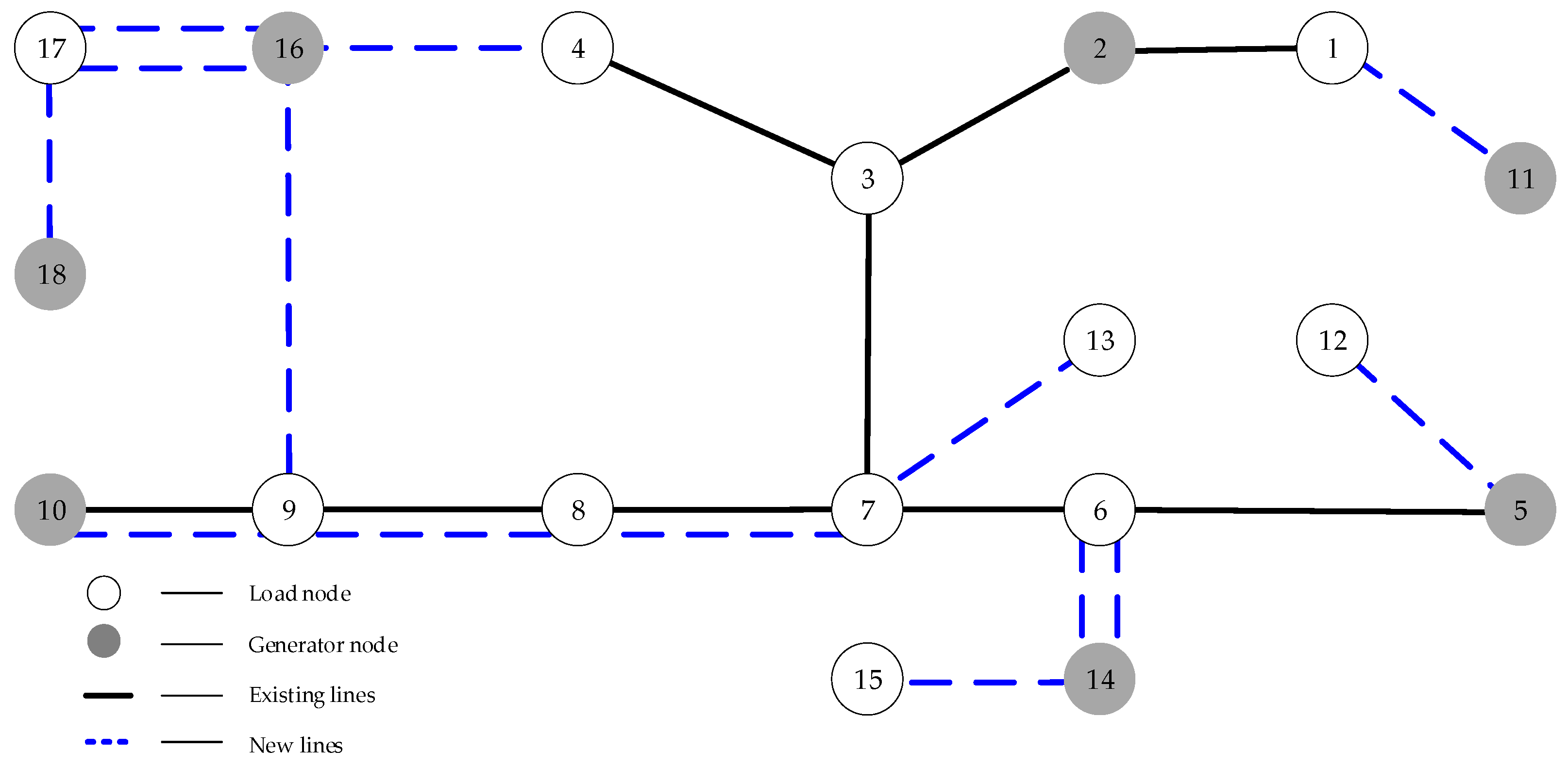
5.1. Planning Grid Analysis

In this paper, a two-layer transmission network planning model considering splitting control is used for transmission network planning, and the results of the planning grid structure are compared with the results of transmission network planning considering the economy. The planning results of the two are shown in Figure 3 and Figure 4, respectively, and the data comparison between the planning results of the two is shown in Table 3. The total investment cost in Table 3 includes lines of construction cost and network loss cost.
Comparison of the planning results of plan 1 and plan 2: 26 new lines have been built in plan 1, with a total investment cost of 26.2 million dollars, while 14 new lines have been built in plan 2, with a total investment cost of 15.7 million dollars. Compared with Figure 1, the total number of new lines and the total investment cost of Figure 2 are less. Although the economy of Figure 1 is slightly worse than that of Figure 2, the grid topology has more ring network structure, which improves the power supply reliability of the system. According to the data in Table 1, Figure 1 will hardly have line overload when operating under normal conditions and N-1 conditions, and it can operate more stably when the system is disturbed by the external environment, which can effectively reduce the line overload accident loss, and the overload loss of option 2 is much larger than that of option 1. In the long run, it can make up the difference in investment cost between option 1 and option 2. Moreover, as shown in Figure 3, the planned grid structure of Figure 1 can be divided into three areas: generators 2, 5 and 11 are in the same area, generators 10, 16 and 18 are in the same area, generators 14 are in another area, and the number of weak connection lines between the areas is 6, respectively lines 2–3, 5–6, 4–16, 9–10, 9–16 and 12–13. The grid structure planned in Figure 2 is shown in Figure 4, which can be divided into four areas. Generators 2 and 11 are in the same area, generators 16 and 18 are in the same area, generators 10, 14 and 5 are in the same area, respectively, and the number of weak connection lines between areas is 4, which are lines 2–3, 4–16, 5–6 and 9–16, respectively. Although Figure 1 has more weakly connected lines than Figure 2, the weak connection coefficient of the system is slightly smaller, and Figure 1 has fewer slow mode partitions and less potential oscillation modes. Overall, Figure 1 has better reliability than Figure 2.

5.2. Feasibility Verification

To verify the feasibility of Figure 1 splitting control in case of serious system failure, this paper simulates Figure 1 in PSD-BPA. The line fault is set as a three-phase short circuit fault, the fault start time is 0s, and the fault duration is 1s. The simulation adopts the generator model and the constant power load model, which take into account the change of magnetic flux, Eq’ and Ed.’

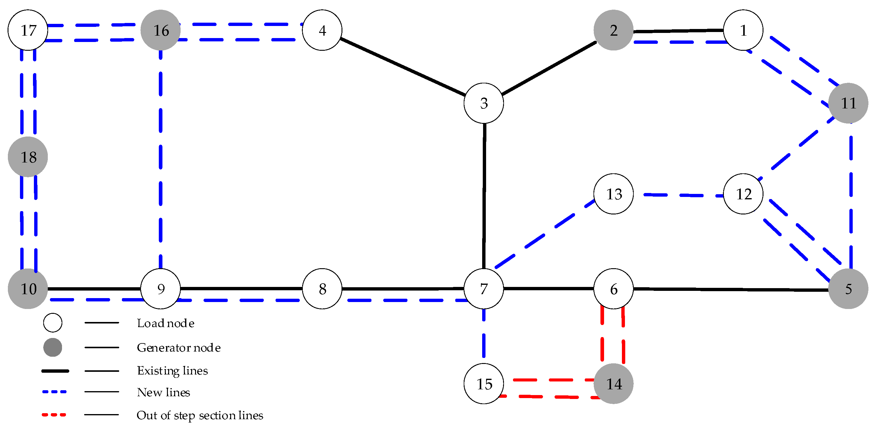
5.2.1. When there is a Fault at the Weak Connection Lines of the System

A fault is set at the front end of the weak connection line 2–3 of the planned grid structure in Figure 1, and the power angle curve of the generator after the fault is shown in Figure 5. As can be seen from Figure 5, when the fault occurs in line 2–3, the power angle of the generator in the system changes. Generators 2, 5, 11 is a group, generators 10, 16, 18 is a group, and generators 14 is a group alone. According to the results of transmission network planning considering splitting control in Section 5.1, it can be seen that the weak connection lines 2–3, 5–6, 4–16, 9–10, 9–16, and 12–13 can be effectively separated from other clusters by splitting the selected splitting sets. According to the analysis of out-of- step splitting criteria based on the frequency of voltage bus, the actual out-of-step sections are lines 2–3, 3–4, 5–6, 6–14, 7–8, 7–15, 12–13, 14–15. It is proved that the feasibility of splitting the weak connection line, in case of failure at the weak connection lines, and the effectiveness of the model splitting control proposed in this paper.

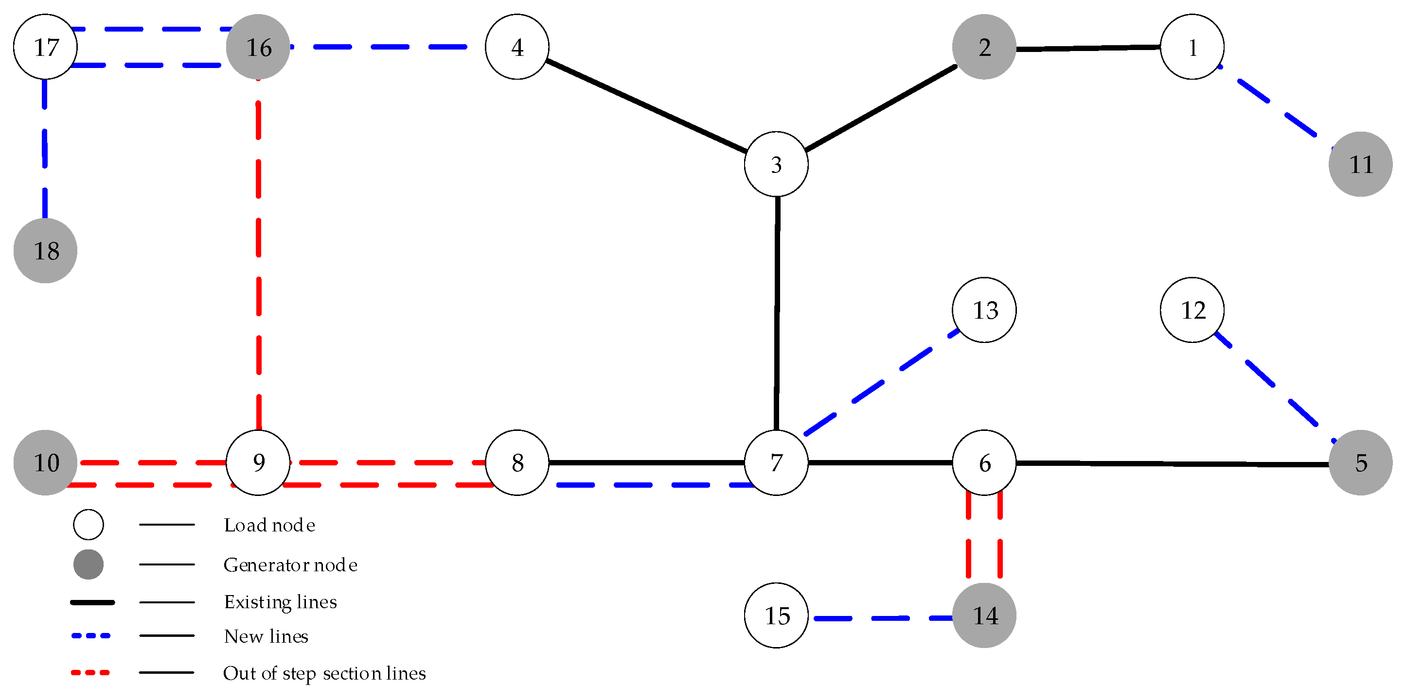
5.2.2. In Case of Internal Line Fault in Slow Mode Area

In Figure 1, faults are set at lines 10–18 of the planned grid structure, and the power angle curve of the generator after faults is shown in Figure 6. As can be seen from Figure 6, when the line 10–18 fails, the system fleet is out-of-step. Generators 2, 5, 11 and 14 are a group, generators 16 and 18 are a group, and generators 10 is a separate group. According to the results of transmission network planning considering splitting control in Section 4.1, splitting at 4–16, 9–10 and 9–16 of the weak connection lines can effectively isolate out-of-step clusters from other clusters, to further find the most suitable splitting section to narrow the search scope and save search time. Through the out-of-step splitting criterion based on the frequency of voltage bus, it is found that the actual oscillation center migrates on lines 3–4, 4–16, 8–9, 9–10, 9–16, 10–18 and 16–17, which verifies the feasibility of taking the weak connection line as the lines to be selected for splitting in case of internal line fault in slow mode area and the effectiveness of the model splitting control proposed in this paper.
The above two sets of simulation verify the feasibility of taking the weak connection lines of the system as the lines to be selected for splitting and prove that the grid structure of the transmission network planning model proposed in this paper can cooperate with the splitting device to quickly partition the system in case of serious complex fault, avoid the spread of oscillation, reduce the search range and time of the optimal splitting section, and cooperate with the splitting control effectively carrying it out.

5.3. Fault Simulation Comparison

To compare the effectiveness of Figure 1 and Figure 2, the N-1 fault simulation of Figure 1 and Figure 2 in PSD-BPA is carried out. The fault setting is the same as that in the feasibility verification. Select a group of fault simulation results for comparison, and take lines 6–14 as fault lines, as shown in Figure 7 and Figure 8:
As can be seen from Figure 7 and Figure 8, the out-of-step section of Figure 1 is concentrated in the area where generators 14 is located; the out-of-step section of Figure 2 is distributed around generators 10 and generators 14. Compared with Figure 1, Figure 2 has a larger distribution area of out-of-step section and more complex oscillation mode when line 6–14 fails. Through the above fault analysis, it can be seen that the out-of-step section of Figure 1 is more concentrated in a certain area compared with Figure 2, which makes the splitting control more accurate and effective.

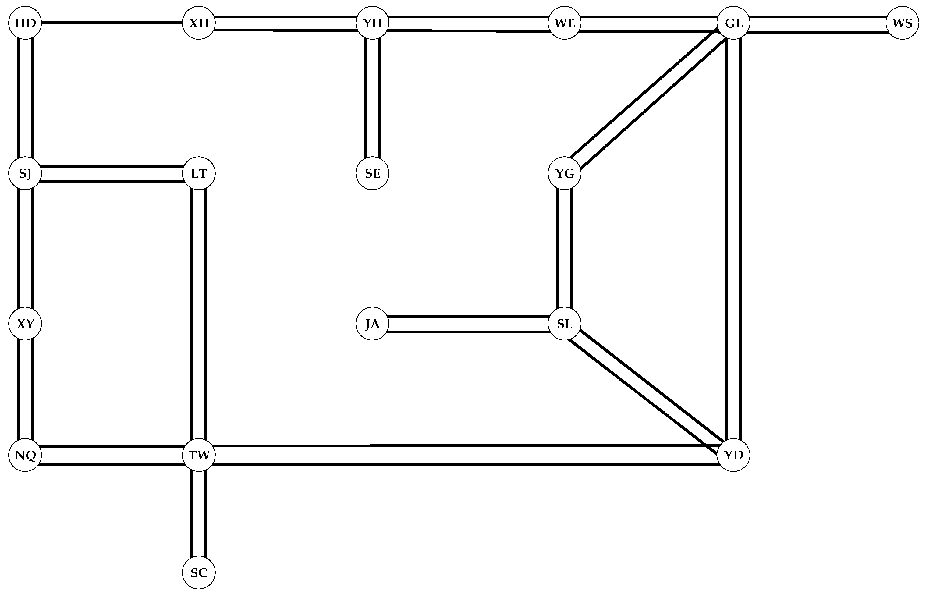
5.4. Simulation of Actual Power Grid

An example of a power grid in East China in the summer of 2018 is used to verify the effectiveness of the proposed power grid planning model. The calculation example includes 812 nodes, 62 generator nodes, and the total load of the system in a certain period is 32,432 MW. The schematic diagram of the power grid transmission line is shown in Figure 9, which can be roughly divided into 14 areas such as XH, HD, SJ, XY, NQ, TW, LT, YD, SL, JA, YG, GL, YH, WE, etc. Based on the transmission network planning model considering splitting control, the planning is carried out based on lines above 500 kV in the grid, and the planned new lines are shown in Table 4.
According to the simulation analysis, the initial grid can be divided into four slow mode areas, with LT and TW as one area, HD, SJ, XY and NQ as one area, and the rest as one area; the weak connection lines of the initial grid are HD-XH, SJ-LT, NQ-TW, LT-TW, and TW-YD respectively. The optimized transmission network planning model considering splitting control is divided into two slow mode areas; TW is one area, and the rest is one area; the weak connection lines of the optimized grid are NQ-TW, LT-TW, and TW-YD. Compared with the original network, the optimized network has less slow mode partition and less weak connection lines.
To verify the effectiveness of the proposed transmission network planning model considering splitting control in the actual grid, three-phase short-circuit fault is set at the GL-YD line of the planning grid, and the initial grid, 0.1 s fault starts, 0.8 s fault duration, and the generator power angle curve is shown in Figure 10 and Figure 11. It can be seen from Figure 10 and Figure 11 that after the initial grid fault, the generators are divided into 4 groups: GL and WE are a group, YD is a group, TW is a group, and the rest of the areas are a group; however, after the optimization of this paper, the generators are divided into 3 groups, among which GL and YD are each a group and other areas are a group. Compared with the optimized grid structure, the initial grid structure has more fault clusters, more complex oscillation modes, and larger distribution areas of out-of-step sections, which can verify the effectiveness of the proposed transmission network planning model considering splitting control in the actual grid.

6. Conclusions

To deal with the increased risk of out-of-step oscillations between regions and improve the ability of interconnected power grid to resist failure risk, this paper proposes a two-level planning model of transmission network considering splitting control, and obtains the following conclusions:
  • Based on the modified cosine factor and graph theory, this paper proposes an improved method of identifying and screening the weak connection lines of the system, which can screen the weak connection lines more accurately and automatically, and does not rely on the judgment of the network topology.
  • Compared with the traditional transmission network planning, this paper proposes the concept of weak connection coefficient of the system and establishes the double-layer planning model of the transmission network with the minimum weak connection coefficient as the optimization goal. The model can optimize the system partition, reduce the decision-making space of the splitting lines, and cooperate with the splitting control rapidly.
  • In this paper, a hybrid algorithm based on Boruvka algorithm and particle swarm optimization algorithm with adaptive mutation and inertia weight is used to solve the IEEE 18 node standard calculation example and a real power grid in East China. Through PSD-BPA fault simulation of the planning results, the feasibility of the weak connection lines as the lines to be selected is verified, and the adaptability of the power grid operation state change is verified. Furthermore, the transmission network planning model proposed in this paper can better cooperate with the splitting control.

Author Contributions

The authors confirm their contributions to the paper as follows: F.T. and C.X. proposed the idea and wrote the paper; X.G. and Y.Z. revised the manuscript; N.D. and B.H. reviewed the results and approved the final version of the manuscript. All authors have read and agreed to the published version of the manuscript.

Funding

This study was funded by the National Natural Science Foundation of China (grant number 51977157).

Acknowledgments

We sincerely thank the editor and the anonymous reviewers of the paper for their kind support. We also want to thank the Grid Corporation for providing relevant information and data.

Conflicts of Interest

The authors declare no conflict of interest.

Nomenclature

Abbreviations
IEEEInstitute of Electrical and Electronics Engineers
PSD-BPAPower System Department—Bonneville Power Administration
N, N-1, N-2, N-Kany K (0, 1, …, K) independent components of the N components of the power system are removed after failure, without damaging the stability of the system.
PSOParticle Swarm Optimization
MWmegawatt
ACAlternating Current
p. u.per unit
XH, HD, SJ, XY, NQ, TW, LT, YD, SL, JA, YG, GL, YH, WE place name
G2, G5, G10, G11, G14, G16, G18generator number
Parameters
Astate matrix
nnumber of generator sets
Ωrated frequency
δirotor angle of generator i
ωispeed of the generator i
Hithe inertia time constant of the generator i
Didamping constant
Pmithe mechanical input power of the generator i
Peithe electromagnetic output of the generator i
Ei, Ejpotential vector amplitude of the generator i and j considering transient reactance
δijpower angle difference between the generator i and j
Gijthe real part of the reduced node admittance matrix of the system
Bijthe imaginary part of the reduced node admittance matrix of the system
Yijreduced node admittance matrix of the system
Pei0generator power steady-state value
δi0generator power angle steady-state value
Ksystem state matrix
Lijclustering matrix
D μ m , min l the lower limit of line sensitivity
D μ m , max l the upper limit of line sensitivity
afund discount rate
rconstruction years
k1line construction cost per unit length
Lilength of line i
mlline set
τiannual loss hours of electric energy of line i
k2unit electricity price
rithe resistance of line i
Uithe voltage of line i
k3unit load cut-off compensation cost
Vi, Vjthe voltage of node i and j
θijphase angle difference between node i and node j
PG,i, QG,iactive power output and reactive power output of node i
PL,i, QL,iactive load and a reactive load of node i
Pijmaxmaximum line capacity
PGgenerator power output
PG, min, PG, maxminimum and maximum generator power output
limaxmaximum number of lines
ωinertia weight
dcurrent particle
c1, c2learning factor
r1, r2random variable between [0,1]
pidindividual extremum
pgdpopulation extremum
pmutation threshold
ηrandom variables obeying [0,1] Gaussian distribution
μrandom variable between [0,1]
ωstart, ωendthe initial and final inertia weight
tmaxmaximum number of iterations
Kconstant
Eq′, Edtransient direct axis and quadrature axis electromotive force
Variables
xsystem state variable
λieigenvalues of the system state matrix
σieigenvalues of second-order systems
μma set of eigenvalues for the system state matrix
mnumber of slow mode eigenvalues
vicharacteristic variables of slow mode eigenvalues
vmomean value of a characteristic variable of slow mode eigenvalue
D λ i l the sensitivity of slow mode eigenvalues λi to line l
ltransmission line
D μ m l the sensitivity of slow mode eigenvalue group to line l
knumber of weak connection lines
F1upper objective function
C1line construction cost
C2network loss cost
C3load shedding cost
F2lower-level objective function
C0weak connection coefficient of the system
Upenalty value for not meeting the lower constraint
linumber of new circuits of line i
Piactive power transmitted by line i
P L N , P L N 1 removal load under N and N-1 conditions
vidparticle velocity
xidparticle position
ωtcurrent inertia weight
titeration times

References

  1. Xiao, C.F.; Tang, F.; Liu, D.C. Power Transmission Network Expansion Planning Research Considering System Weak Connection Recognition. In Proceedings of the 2019 IEEE Innovative Smart Grid Technologies—Asia (ISGT Asia), Chengdu, China, 21–24 May 2019; pp. 191–195. [Google Scholar]
  2. Wu, W.P.; Hu, Z.C. Transmission Network Expansion Planning Based on Chronological Evaluation Considering Wind Power Uncertainties. IEEE Trans. Power Syst. 2018, 33, 4787–4796. [Google Scholar] [CrossRef]
  3. Zhou, Y.; Zhou, Q.M.; Yu, H.Q. Splitting control decision Figure design and splitting control analysis in a provincial power grid. In Proceedings of the 2016 12th World Congress on Intelligent Control and Automation (WCICA), Guilin, China, 12–15 June 2016; pp. 2338–2342. [Google Scholar]
  4. Tang, F.; Yang, J. Out-of-step oscillation splitting criterion based on bus voltage frequency. J. Mod. Power Syst. Clean Energy 2015, 3, 341–352. [Google Scholar] [CrossRef] [Green Version]
  5. Liu, Y.Y. Analysis of Brazilian blackout on 21st March 2018, and revelations to security for human grid. In Proceedings of the 2019 4th International Conference on Intelligent Green Building and Smart Grid (IGBSG), Yichang, China, 6–9 September 2019; pp. 1–5. [Google Scholar]
  6. Licia, P.; Carlos, R.M. The Venezuelan energy crisis: Renewable energies in the transition towards sustainability. Renew. Sustain. Energy Rev. 2019, 105, 415–426. [Google Scholar]
  7. Zhang, S.; Zhang, Y.X. A Novel Out-of-Step Splitting Protection Based on the Wide Area Information. IEEE Trans. Smart Grid 2017, 8, 41–51. [Google Scholar] [CrossRef]
  8. Zhang, S.; Zhang, Y.X. Characteristic Analysis and Calculation of Frequencies of Voltages in Out-of-Step Oscillation Power System and a Frequency-Based Out-of-Step Protection. IEEE Trans. Power Syst. 2019, 34, 205–214. [Google Scholar] [CrossRef]
  9. Stott, B.; Marinho, J.L. Linear programming for power-system network security applications. IEEE Trans. Power App. Syst. 1979, 98, 837–848. [Google Scholar] [CrossRef]
  10. Street, A.; Oliveira, F. Contingency-constrained unit commitment with n-k security criterion: A robust optimization approach. IEEE Trans. Power Syst. 2011, 26, 1581–1590. [Google Scholar] [CrossRef]
  11. Reddy, S.S. Multi-Objective Based Congestion Management Using Generation Rescheduling and Load Shedding. IEEE Trans. Power Syst. 2017, 32, 852–863. [Google Scholar]
  12. Kroposki, B.; Sen, P.K. Optimum sizing and placement of distributed and renewable energy sources in electric power distribution systems. IEEE Trans. Ind. Apps. 2013, 49, 2741–2752. [Google Scholar] [CrossRef]
  13. Sajad, N.R.; Nazanin, J. Smart distribution grid multistage expansion planning under load forecasting uncertainty. IET Gener. Transm. Distrib. 2016, 10, 1136–1144. [Google Scholar]
  14. Li, Z.H.; Lin, Y.; Chen, W.H. Fuzzy comprehensive evaluation for transmission grid planning based on combination weight. In Proceedings of the International Conference on Power and Energy, CPE 2014, Shanghai, China, 29–30 November 2014; pp. 91–96. [Google Scholar]
  15. Yorino, N.; Abdillah, M. Robust Power System Security Assessment Under Uncertainties Using Bi-Level Optimization. IEEE Trans. Power Syst. 2017, 33, 352–362. [Google Scholar] [CrossRef]
  16. Tan, K.M.; Ramachandaramurthy, V.K. Optimal vehicle to grid planning and scheduling using double layer multi-objective algorithm. Energy 2016, 112, 1060–1073. [Google Scholar] [CrossRef]
  17. Ni, J.M.; Shen, C. An on-line weak-connection identification method for controlled islanding of power system. Proc. Chinese Soc. Electr. Eng. 2011, 31, 24–30. [Google Scholar]
  18. Yang, Y.G.; Duan, Q.G.; Wu, G.B. Slow coherency based adaptive controlled islanding Figure of the China Southern Power Grid. In Proceedings of the 2015 IEEE PES Asia-Pacific Power and Energy Engineering Conference (APPEEC), Brisbane, Australia, 15–18 November 2015; pp. 1–5. [Google Scholar]
  19. Li, M.X. An improved fcm clustering algorithm based on cosine similarity. In Proceedings of the 2019 International Conference on Data Mining and Machine Learning, ICDMML 2019, Hong Kong, China, 28–30 April 2019; pp. 103–109. [Google Scholar]
  20. Ma, Z.Y.; Liu, F. Fast Searching Strategy for Critical Cascading Paths Toward Blackouts. IEEE Access 2018, 6, 36874–36886. [Google Scholar] [CrossRef]
  21. Alinezhad, B.; Karegar, H.K. Out-of-Step Protection Based on Equal Area Criterion. IEEE Trans. Power Syst. 2017, 32, 968–977. [Google Scholar] [CrossRef]
  22. Song, H.L.; Wu, J.Y. A wide-area measurement systems-based adaptive strategy for controlled islanding in bulk power systems. Energies 2014, 7, 2631–2657. [Google Scholar] [CrossRef] [Green Version]
  23. Kokotovic, P.V.; Avramovic, B. Coherency based decomposition and aggregation. Automatica 1982, 18, 47–56. [Google Scholar] [CrossRef]
  24. Chow, J.H.; Kokotovic, P.V. Decomposition of near-optimum regulators for systems with slow and fast modes. IEEE Trans. Autom. Control 1976, 21, 701–705. [Google Scholar] [CrossRef]
  25. Yang, B.; Vittal, V. Slow-Coherency-Based Controlled Islanding—A Demonstration of the Approach on the August 14, 2003 Blackout Scenario. IEEE Trans. Power Syst. 2006, 21, 1840–1847. [Google Scholar] [CrossRef]
  26. Wang, X.M.; Vittal, V. Tracing generator coherency indices using the continuation method: A novel approach. IEEE Trans. Power Syst. 2005, 20, 1510–1518. [Google Scholar] [CrossRef]
  27. Ni, J.M.; Shen, C. Adaptive islanding control based on slow coherency-Part II: Practical area partition method. Proc. Chinese Soc. Electr. Eng. 2014, 34, 4865–4875. [Google Scholar]
  28. Xu, G.Y.; Vittal, V. Slow Coherency Based Cutset Determination Algorithm for Large Power Systems. IEEE Trans. Power Syst. 2010, 25, 877–884. [Google Scholar] [CrossRef]
  29. Seo, J.H.; Im, C.H. Multimodal function optimization based on particle swarm optimization. IEEE Trans. Magn. 2006, 42, 1095–1098. [Google Scholar] [CrossRef]
  30. Zhang, J.T.; Xia, P.Q. An improved PSO algorithm for parameter identification of nonlinear dynamic hysteretic models. J. Sound Vibr. 2017, 389, 153–167. [Google Scholar] [CrossRef]
Figure 1. Schematic diagram of the slow mode area.
Sustainability 12 01769 g001
Figure 2. Flow chart for solving bi-level programming model of transmission network considering splitting control.
Sustainability 12 01769 g002
Figure 3. Planning results of the transmission network considering splitting control.
Sustainability 12 01769 g003
Figure 4. Planning results of the transmission network considering the economy.
Sustainability 12 01769 g004
Figure 5. Generator power angle curve in case of line 2–3 fault.
Sustainability 12 01769 g005
Figure 6. Generator power angle curve in case of line 10–18 fault.
Sustainability 12 01769 g006
Figure 7. Out-of-step section of Figure 1 in case of line 6-14 failure.
Sustainability 12 01769 g007
Figure 8. Out-of-step section of Figure 2 in case of line 6–14 failure.
Sustainability 12 01769 g008
Figure 9. Schematic diagram of the transmission line for a power grid in East China.
Sustainability 12 01769 g009
Figure 10. Power angle curve of the generator after line GL-YD fault of the initial grid structure.
Sustainability 12 01769 g010
Figure 11. Power angle curve of the generator after line GL-YD fault of the optimized grid structure.
Sustainability 12 01769 g011
Table 1. IEEE 18 node system network node parameters.
NodeGenerator Output (MW)Load (MW)
1055
236084
30154
4038
5760639
60199
70213
8088
90259
1075094
11540700
120190
130110
1454032
150200
16495132
170400
181420
Table 2. IEEE 18 node system network branch parameters.
Number of LineEnds NodeAC Resistance (p.u.)AC reactance
(p.u.)
Length (km)Capacity (MW)Number of Existing LinesNumber of Lines That Can be Built
11–20.0010.01767023013
21–110.0010.01024023003
32–30.0010.034813823013
43–40.0010.040415523013
53–70.0010.032512923013
64–70.0010.050120023003
74–160.0010.050120023003
85–60.0010.026710623013
95–110.0010.01536023003
105–120.0010.01024023003
116–70.0010.01265023013
126–130.0010.01265023003
136–140.0010.055422023003
147–80.0010.01516023013
157–90.0010.031812623003
167–130.0010.01265023003
177–150.0010.044817823003
188–90.0010.01024023013
199–100.0010.050120023013
209–160.0010.050120023003
2110–180.0010.025510023003
2211–120.0010.01265023003
2311–130.0010.025510023003
2412–130.0010.01536023003
2514–150.0010.042817023003
2616–170.0010.01536023003
2717–180.0010.01405523003
Table 3. Comparison of transmission network planning results considering splitting control and economy.
Planning FigureFigure 1: Transmission Network Planning Results Considering Splitting ControlFigure 2: Transmission Network Planning Results Considering the Economy
Number of new lines and circuits1–2(1), 1–11(2)
4–16(2), 5–11(1)
5–12(2), 6–14(2)
7–8(1), 7–13(1)
7–15(1), 8–9(1)
9–10(1), 9–16(1)
10–18(2), 11–12(1)
12–13(1), 14–15(2)
16–17(2), 17–18(2)
1–11(1), 4–16(1)
5–12(1), 6–14(2)
7–8(1), 8–9(1)
7–13(1), 9–10(1)
9–16(1), 14–15(1)
16–17(2), 17–18(1)
Total investment cost/106 $26.215.7
Load shedding cost/104 $01.27
N-1 load shedding cost/104 $0.0688.67
Weak connection coefficient0.1710.173
Table 4. Planning new lines.
FigureNumber of New Lines and Circuits
Transmission network planning results considering splitting controlHD-SJ (1), HD-XH (1), SJ-XY (1)
XY-NQ (1), SL-JA (1), GL-YD (1)

