Probabilistic Assessment of Distribution Network with High Penetration of Distributed Generators

Abstract

Over the past decades, the deployment of distributed generations (DGs) in distribution systems has grown dramatically due to the concerns of environment and carbon emission. However, a large number of DGs have introduced more uncertainties and challenges into the operation of distribution networks. Due to the stochastic nature of renewable energy resources, probabilistic tools are needed to assist systems operators in analyzing operating states of systems. To address this issue, we develop a probabilistic framework for the assessment of systems. In the proposed framework, the uncertainties of DGs outputs are modeled using short term forecast values and errors. Moreover, an adaptive cluster-based cumulant method is developed for probabilistic load flow calculation. The performance of the proposed framework is evaluated in the IEEE 33-bus system and PG&E 69-bus system. The results indicate that the proposed framework could yield accurate results with a reasonable computational burden. The excellent performance of the proposed framework in estimating technological violations can help system operators underlying the potential risks of systems.

1. Introduction

The increased concerns over carbon dioxide emission and energy saving have led to the drastic integration of DGs into the distribution networks [1,2]. The strategical deployment integration of DGs brings some technical and economic benefits [3], including improvement of voltage profile [4], reduction of power loss [5], and enhancement of system reliability [6]. However, the excessive penetration of DGs introduces more uncertainties into the systems and may alter the normal operational behavior of distribution networks. For instance, overvoltage and overloading [7,8] may occur during the periods of high DGs generation and low load demand. Therefore, probabilistic analysis tools are needed to achieve a better understanding of the technical impacts of DGs.

Probabilistic load flow (PLF) [9], as a probabilistic analysis tool, has been widely used in identifying and quantifying potential risks since it was proposed in 1974. From a mathematical point of view, the calculation of PLF is essentially a process of estimating the probability distribution of functions of multiple random variables [10]. The authors in [11] presented a comprehensive review of the methods of PLF calculations. These methods could be classified into three main categories: numerical methods [12,13,14,15,16], approximate methods [17,18,19,20], and analytical methods [21,22,23,24,25]. The above methods [12,19,22] have been widely applied to evaluate the impact of DGs on distributions networks.

Monte Carlo simulation (MCS) is a well-known numerical method for PLF calculation. MCS relies on a significant number of samples and repetitive load flow calculations to harvest accurate results. In [12,13], MCS-based PLF was used for the assessment of DGs impacts in distribution networks. Although this method can yield accurate results, the large computational burden hinders its application in practical systems. In order to achieve acceptable efficiency, some efficient sampling techniques have been established. For instance, the authors in [14] adopted Latin Hypercube Sampling (MCS-LHS) based PLF to analyze the overvoltage issue of distribution systems with the large integration of photovoltaics (PVs). The occurrence of overvoltage was compared with or without voltage control algorithm. Sophisticated sampling methods [15,16] can reduce the number of load flow calculations. However, the efficiency of MCS is still low, especially in large scale systems.

Approximate methods require less computational time compared with MCS. The representative methods in this category are the point estimate methods (PEMs) [17]. PEMs approximate the statistical moments of output variables through the load flow calculations at a few representative operating states. Based on the selection of operating states, PEMs can be classified as 2m, 2m + 1, 3m, and 4m + 1 schemes, where m represents the number of input variables. A comparison of various schemes of PEMs was presented in [18]. The results indicated that the 2m + 1 PEM provides the best solution in terms of accuracy and computational burden. The authors in [19] adopted 2m+1 PEM to analyze voltage unbalance in distribution networks with single-phase PVs. The probabilistic assessment of distribution systems with PVs and electric vehicles (EVs) was performed in [20] using 2m+1 PEM. PEMs can obtain accurate results with reasonable computational efficiency when the number of the input variable is relatively small. However, the computational burden of PEMs is linearly related to the number of input variables. Moreover, PEMs hold lower accuracy in estimating higher-order moments of output variables [11].

Analytical methods generally adopt the linearized load flow model. As a representative analytical method, the cumulant method [21] only performs one load flow calculation and obtains cumulants of outputs from the cumulant of inputs through a simple linear transformation. Then, some reconstruction techniques (e.g., expansion series [21,22]) were used to recover the probability distributions of outputs. The combined cumulant method with the Cornish-Fisher expansion series was proposed in [22] to solve the PLF problem of radial distribution systems with PVs. Moreover, cumulant method was extended to assess the impact of PVs [23] and other low carbon technologies (e.g., EVs [24] and biomass-fueled gas engines [25]) on the behaviors of distribution networks. Cumulant method is suitable for large systems with multiple inputs since its computational burden is low. However, due to the adoption of the linearized load flow model, the accuracy of the cumulation-based method decreases when dealing with input variables with significant variations.

It is clear from the brief review that a vast body of literature has performed assessments of distribution networks with the integrations of DGs. These studies have contributed significantly to understand the behaviors of distribution networks in the presence of uncertainties. However, two challenges remain to be addressed for the probabilistic assessment in distribution networks. First, in previous studies [15,18], researchers adopted Weibull distribution to represent the variations of wind speed. This assumption can be reasonable for the distribution of wind speed over a long time scale. Moreover, some studies [13,24] focused on the aggregated statistical impact of DGs on systems over a long time scale. However, less work has been done on the evaluation of distribution networks over a short time scale. For distribution network operators (DNOs), it is more valuable to understand the behaviors of systems over short time scales and to predict potential risks of operating states. Second, the integration of a large number of DGs introduces significant uncertainties to the systems, which calls for the PLF methods with higher accuracy and less computational time. From the perspective of computational burden, the cumulant-based methods seem to be adequate due to the relatively less number of load flow calculations required. However, the adaptation of linearized load flow equations makes the method less accurate in the case of a high level of uncertainties.

Motivated by the research gap and challenges, this study aims to develop a probabilistic framework for the assessment of distribution networks with a large number of DGs. To address the first challenge, we take advantage of short term forecast values and corresponding forecast errors [26,27] to model the uncertainties of DGs output. By establishing the probability distributions of DGs outputs in each time period, e.g., 15-min, the behaviors of systems in a short time scale can be captured. For the second challenge, we develop an adaptive cluster-based cumulant method for PLF calculation. With the use of the K-means clustering technique, the proposed method overcomes the shortcomings of the conventional cumulant method in computational accuracy. Compared with existing studies [28,29], the main feature of the proposed method is the adaptive scheme for the determination of clusters number. The performance of the proposed framework is evaluated in the IEEE 33-bus system and PG&E 69-bus system with wind power DGs. The results demonstrate that the framework can achieve high accuracy in estimating probability distributions and potential risk with a reasonable computational burden.

The paper is organized as follows. Section 2 presents the modeling of wind power outputs using short term forecast values and errors. Section 3 presents the traditional cumulant method, K-means clustering technique, and the proposed adaptive cluster-based cumulant method for PLF calculation. Section 4 performs the numerical studies on the IEEE 33-bus and PG&E 69-bus system to evaluate the performance of the proposed framework. Finally, Section 5 summarizes the main conclusions of this study.

2. Modeling of Uncertainty

In this section, we adopt short term forecast values and errors to model the uncertainties of renewable energy output. Note that the proposed method can assess the impacts of wind power, PVs, and hybrid wind power-PVs on systems. This study only focuses on wind power to simplify the description.

The stochastic nature of wind power and load demand makes the operating state assessment of distribution networks challenging. The premise of accurate evaluation results is accurate uncertainty modeling. Load demand is highly time-dependent and comprises of both deterministic and random components. The random part arises from forecasting and measurement errors. Moreover, Gaussian distribution [11] can provide a reasonable representation of the uncertainties of load demands since the variation is not too large. For wind power, the outputs of wind farms mainly depend on wind speed and direction. Some studies [15,18] adopted Weibull distributions to represent the uncertainty of wind speed. This assumption is reasonable for the distribution of wind speed in some areas over a long time scale. However, there lacks evidence that the Weibull distribution is applicable to model wind speed over a short time scale, e.g., 15-min. In this context, short term forecast values and errors can provide an alternative to represent the stochastic nature of wind power.

The short term forecast of wind power is usually conducted on a day-ahead basis. It provides system operators with the estimations of wind power outputs for the next day. Based on the forecast information, the system operator can determine the generation plans for the next day. Figure 1 presents a 5-day snapshot of historical data of forecast and real powers. The resolution of the data set is 15-min. Therefore, this data set has a total of 480 data points. The forecast values are obtained by point forecast tool, i.e., the forecast power is a deterministic value in each period. However, due to the stochastic nature of wind speed and direction, there are deviations between the forecast and real powers. In this case, the actual wind power output p_w,r can be represented as the superposition of its forecast value p_w,f and corresponding error p_w,e, as follows:

$$p_{w,r}=p_{w,f}+p_{w,e}$$

(1)

Consider the forecast error of a single wind farm, the historical data sets of forecast and actual power can be expressed as ${\mathit{P}}_{w,f}=[p_{w,f}^1,...,p_{w,f}^i,...p_{w,f}^m]$ and ${\mathit{P}}_{\omega ,r}=[p_{w,r}^1,...,p_{w,r}^i,...p_{w,r}^m]$, respectively. The data sets consist of m data points. The correlation between the forecast data and the actual data can be modeled using the copula function [26,30], as follows:

$$F_{{\mathit{P}}_{w,r}}{,}_{{\mathit{P}}_{w,f}}(p_{w,r}^i,p_{w,f}^i)=C(F_{{\mathit{P}}_{w,r}}(p_{w,r}^i),F_{{\mathit{P}}_{w,f}}(p_{w,f}^i))$$

(2)

where $F_{{\mathit{P}}_{w,r}}{,}_{{\mathit{P}}_{w,f}}(p_{w,r}^i,p_{w,f}^i)$ is the joint distribution of variables P_w,r and P_w,f; $F_{{\mathit{P}}_{w,r}}(p_{w,r}^i)$ and $F_{{\mathit{P}}_{w,f}}(p_{w,f}^i)$ are the marginal distribution of P_w,r and P_w,f, respectively; $C(\cdot )$ is the copula function.

According to (2), the joint probability density function (PDF) of the forecast data and the actual data can be written as:

$$f_{{\mathit{P}}_{w,r}}{,}_{{\mathit{P}}_{w,f}}(p_{w,r}^i,p_{w,f}^i)=c(F_{{\mathit{P}}_{w,r}}(p_{w,r}^i),F_{{\mathit{P}}_{w,f}}(p_{w,f}^i))\cdot f_{{\mathit{P}}_{w,r}}(p_{w,r}^i)\cdot f_{{\mathit{P}}_{w,f}}(p_{w,f}^i)$$

(3)

where $f_{{\mathit{P}}_{w,r}}{,}_{{\mathit{P}}_{w,f}}(p_{w,r}^i,p_{w,f}^i)$ is the joint PDF of P_w,r and P_w,f; and $f_{{\mathit{P}}_{w,f}}(p_{w,f}^i)$ are the marginal PDFs of P_w,r and P_w,f, respectively; $c(\cdot )$ is the copula density function.

Given the short term forecast power at t time period p_w,f,t the conditional PDF of real power can be represented as:

$$\begin{array}{ll}{f}_{{\mathit{P}}_{w,r}|p_{w,f,t}}(p_{w,r}^i|p_{w,f}^i=p_{w,f,t})& =\frac{f_{{\mathit{P}}_{w,r}}{,}_{{\mathit{P}}_{w,f}}(p_{w,r}^i,p_{w,f,t})}{f_{{\mathit{P}}_{w,f}}(p_{w,f,t})}\\ & =c(F_{{\mathit{P}}_{w,r}}(p_{w,r}^i),F_{{\mathit{P}}_{w,f}}(p_{w,f,t}))\cdot f_{{\mathit{P}}_{wind,r}}(p_{w,r}^i)\hfill \end{array}$$

(4)

According to Equations (1) and (4), the conditional PDF of forecast error can be expressed as follows:

$$\begin{array}{ll}{f}_{p_{w,e,t}|p_{w,f,t}}(p_{w,e,t}|p_{w,f}^i=p_{w,f,t})& =\frac{f_{{\mathit{P}}_{w,r}}{,}_{{\mathit{P}}_{w,f}}(p_{w,r}^i,p_{w,f,t})}{f_{{\mathit{P}}_{w,f}}(p_{w,f,t})}\\ & =c(F_{{\mathit{P}}_{w,r}}(p_{w,e,t}+p_{w,f,t}),F_{{\mathit{P}}_{w,f}}(p_{w,f,t}))\cdot f_{{\mathit{P}}_{wind,r}}(p_{w,e,t}+p_{w,f,t})\hfill \end{array}$$

(5)

The upper and lower bounds of the forecast error p_w,e,t are max(P_w,r)-p_w,f,t and -p_w,f,t, respectively.

As shown in (5), the estimation of forecast errors requires two elements, i.e., historical data sets and the copula function that used to represent the dependence between forecast and actual power. The optimal copula function (e.g., Gaussian copula) can be obtained by the method in [30]. Given the short term forecast values of different periods, the corresponding probability distributions of forecast errors can be calculated by arithmetic operations. Moreover, (5) can be extended to model the forecast errors of multiple wind farms. Under such circumstances, the multivariate copula function is required to represent the multidimensional correlations.

3. Probabilistic Assessment Framework

This section introduces the proposed framework for the probabilistic assessment. First, a theoretical background of the traditional cumulant method (TCM) is presented. Second, the K-means clustering technique is introduced to group samples of wind power into serval clusters. Then, the adaptive cluster-based cumulant method (ACCM) is proposed. Finally, the computational procedure of the proposed framework is presented.

3.1. Traditional Cumulant Method for PLF

The nonlinear load flow equations of power systems can be represented as follows:

$$\{\begin{array}{l}\mathit{W}=\mathit{f}(\mathit{X})\\ \mathit{Z}=\mathit{g}(\mathit{X})\end{array}$$

(6)

where W represents the vector of input variables (injected active and reactive power); X is the vector of state variables (voltage magnitudes and angles); Z denotes the vector of output variables (active and reactive powers); and f(·) and g(·) are the nonlinear load flow functions.

The load flow equations can be linearized around a working point in terms of Taylor’s series, and the high-order term of 2 times and above are ignored, as follows:

$$\{\begin{array}{ll}\mathit{W}& =\mathit{f}(\mathit{X})={\mathit{W}}_0+\mathrm{\Delta }\mathit{W}\\ & =\mathit{f}({\mathit{X}}_0+\mathrm{\Delta }\mathit{X})\approx f({\mathit{X}}_0)+{\mathit{J}}_0\mathrm{\Delta }\mathit{X}\\ \mathit{Z}& =\mathit{g}(\mathit{X})={\mathit{Z}}_0+\mathrm{\Delta }\mathit{Z}\\ & =\mathit{g}({\mathit{X}}_0+\mathrm{\Delta }\mathit{X})\approx \mathit{g}({\mathit{X}}_0)+{\mathit{G}}_0\mathrm{\Delta }\mathit{X}\end{array}$$

(7)

where ΔW, ΔX, and ΔZ are the variations of random variables W, X, and Z, respectively; J₀ and G₀ can be calculated as follows:

$$\{\begin{array}{l}{\mathit{J}}_0=\partial \mathit{f}(\mathit{X})/\partial \mathit{X}|{}_{\mathit{X}={\mathit{X}}_0}\\ {\mathit{G}}_0=\partial \mathit{g}(\mathit{X})/\partial \mathit{X}|{}_{\mathit{X}={\mathit{X}}_0}\end{array}$$

(8)

According to (7), the relationship among input, state, and output random variables at the reference point can be expressed as follows:

$$\{\begin{array}{l}\mathrm{\Delta }\mathit{X}={\mathit{J}}_0^{-1}\mathrm{\Delta }\mathit{W}={\mathit{S}}_0\mathrm{\Delta }\mathit{W}\\ \mathrm{\Delta }\mathit{Z}={\mathit{G}}_0{\mathit{J}}_0^{-1}\mathrm{\Delta }\mathit{W}={\mathit{T}}_0\mathrm{\Delta }\mathit{W}\end{array}$$

(9)

Cumulant method [22] can be used to obtain the probability distributions of state and output variables based on the linear relationship in (9). The cumulants of input variables can be calculated as follows:

$${\gamma }_{\mathit{W}}^r=\{\begin{array}{ll}{\alpha }_{\mathit{W}}^1& (r=1)\\ {\alpha }_{\mathit{W}}^r-{\displaystyle \sum _{i=1}^{r-1}}{C}_{r-1}^i{\alpha }_{\mathit{W}}^i{\gamma }_{\mathit{W}}^{r-i}& (r>1)\end{array}$$

(10)

where ${\alpha }_{\mathit{W}}^r$ and ${\gamma }_{\mathit{W}}^r$ are the r-th order moments and cumulant of input variables W, respectively.

Based on the properties of cumulant [31], the cumulants of state and output variables can be calculated by the linear combination of input cumulants:

$$\{\begin{array}{l}{\gamma }_{\mathit{X}}^r=({\mathit{J}}_0^{-1}{)}^r{\gamma }_{\mathit{W}}^r=({\mathit{S}}_0{)}^r{\gamma }_{\mathit{W}}^r\\ {\gamma }_{\mathit{Z}}^r=({\mathit{G}}_0{\mathit{J}}_0^{-1}{)}^r{\gamma }_{\mathit{W}}^r=({\mathit{T}}_0{)}^r{\gamma }_{\mathit{W}}^r\end{array}$$

(11)

where ${\gamma }_{\mathit{X}}^r$ and ${\gamma }_{\mathit{Z}}^r$ are the r-th order cumulants of variables X and Z, respectively.

When the cumulants of state and output variables are obtained, the series expansion techniques, such as the Gram–Charlier series expansion [21] and Cornish–Fisher series expansion [22] can be used to obtain the probability distribution. This paper adopts the Cornish–Fisher series expansion to obtain the probability distribution of variables due to its better performance in approximating non-Gaussian distribution. A detailed mathematical description of series expansion techniques can be found in [22].

It can found from the description above that TCM has moderate steps to solve the PLF problem. More importantly, TCM only requires one load flow calculation. Therefore, it has high computational efficiency. However, the assumption of linearized load flow can introduce some errors. Moreover, the errors are more notable when the fluctuations of input variables are relatively large. In this context, one solution to address this disadvantage is to use clustering techniques to partition the variation of input variables.

3.2. Data Clustering Algorithm

Before the introduction of clustering technology, the samples of wind power need to be generated. Assume that M wind farms are integrated into the system, and the probability distribution of each wind power output at period t can be obtained using the technique in Section 2. The dependence of wind powers is represented using the correlation matrix. The LHS technique and Nataf transformation [15] is adopted to generate samples of wind power outputs. The samples matrix of wind powers can be represented as follows:

$$\begin{array}{ll}{W}_{M\times N}& =[{\omega }_1,{\omega }_2,...,{\omega }_i,...,{\omega }_N]\\ & =\left[\begin{array}{ccc}\begin{array}{c}{w}_{11}\\ ⋮\end{array}& \begin{array}{c}{w}_{12}\\ ⋮\end{array}& \begin{array}{cc}\begin{array}{cc}\begin{array}{cc}\begin{array}{c}...\\ ...\end{array}& \begin{array}{c}{w}_{1i}\\ ⋮\end{array}\end{array}& \begin{array}{c}...\\ ...\end{array}\end{array}& \begin{array}{c}{w}_{1N}\\ ⋮\end{array}\end{array}\\ w_{l1}& w_{l2}& \begin{array}{cc}\begin{array}{cc}\begin{array}{cc}...& w_{li}\end{array}& ...\end{array}& w_{lN}\end{array}\\ \begin{array}{c}⋮\\ w_{M1}\end{array}& \begin{array}{c}⋮\\ w_{M2}\end{array}& \begin{array}{cc}\begin{array}{cc}\begin{array}{cc}\begin{array}{c}\\ ...\end{array}& \begin{array}{c}⋮\\ w_{Mi}\end{array}\end{array}& \begin{array}{c}\\ ...\end{array}\end{array}& \begin{array}{c}⋮\\ w_{MN}\end{array}\end{array}\end{array}\right]\end{array}$$

(12)

where ${\omega }_i=[w_1,...,w_i,...,w_M{]}^T$; variable N represents the sample size.

Based on the samples of wind power, this paper adopts the K-means algorithm to group the wind powers into serval clusters. Data clustering is the process of grouping a set of data based on its characteristics. K-means clustering technique has been widely used in many aspects of the power systems [32,33], and it proved to be an efficient way to realize the classification of data. K-means algorithm aims to find the optimal cluster centers to minimize the sum of the Euclidean distance between all data points and the cluster centers. The objective of K-means clustering can be written as:

$$\min {\displaystyle \sum _{j=1}^K{\displaystyle \sum _{i=1}^{n_j}{\Vert {\mathit{\omega }}_i-{\mathit{c}}_j\Vert }^2}}$$

(13)

where k is the number of clusters; ${\mathit{c}}_j$ is the cluster center of cluster j; ${\mathit{\omega }}_i$ the i-th data point in cluster j; $n_j$ is the total number of data points in cluster j.

The computational steps of K-means algorithm are as follows:

Step 1: Determine the number of clusters K;

Step 2: Random select K data points from the whole data set as initial cluster centers;

Step 3: Allocate the remained data points to the clusters with the closest Euclidean distance:

$$\begin{array}{l}if\hspace{1em}\left|{\omega }_k-{\mathit{c}}_j\right|<\left|{\omega }_k-{\mathit{c}}_h\right|\Rightarrow {\omega }_k\in {\mathit{C}}_j\\ k=1,2,...,N\hspace{1em}\hspace{1em}j,h=1,2,...,K\end{array}$$

(14)

where c_j and c_h are the cluster centers of cluster j and h; C_j is the set of cluster j; ω_k is the k-th data point in raw data set; N is the total number of data points in the raw data set.

Step 4: Update the cluster centers as follows:

$${\mathit{c}}_j=\frac{{\displaystyle {\sum }_{i\in {\mathit{C}}_j}{\omega }_i}}{n_j}\hspace{1em}j=1,2,...,K$$

(15)

Step 5: Repeat step 3 and 4 until the variation of cluster centers less than the preset threshold;

Step 6: Calculate the occurrence probability of the j-th cluster as follows:

$$p_j=\frac{n_j}{N}\hspace{1em}\hspace{1em}j=1,2,...,K$$

(16)

Figure 2 shows an example of clustering the outputs of two wind farms, in which the wind powers are categorized into eight clusters. It can be observed from Figure 2a that the variation interval of the original data set of wind power 1 is [0.3 p.u, 1.0 p.u]. In contrast, the wind power fluctuation of each cluster in Figure 2b is much smaller than that of the whole data set. As mentioned in Section 3.1, the accuracy of TCM decreases when dealing with the input variable with relatively large variations. Therefore, using K-means clustering to reduce the fluctuation of input variables can alleviate the disadvantage of TCM.

3.3. Adaptive Cluster-Based Cumulant Method for PLF

In Section 3.2, the raw data set of wind power is categorized into K clusters using the K-means algorithm. For each cluster, wind power varies within a smaller range. In this context, the cumulant method (7)–(10) can be used to obtain the probability distribution of the state and output variables. For cluster j, the variations of state and output variables can be calculated as follows:

$$\mathrm{cluster} j:\{\begin{array}{l}\Delta {\mathit{X}}_j={\mathit{J}}_{0j}^{-1}\Delta {\mathit{W}}_j={\mathit{S}}_{0j}\Delta {\mathit{W}}_j\\ \Delta {\mathit{Z}}_j={\mathit{G}}_{0j}{\mathit{J}}_{0j}^{-1}\Delta \mathit{W}j={\mathit{T}}_{0j}\Delta {\mathit{W}}_j\end{array}$$

(17)

where ΔW_j is the variations of input variables in the j-th cluster; ΔX_j andΔZ_j are the variations of the state and output variables in the j-th cluster.

Accordingly, the cumulant of state and output variables with cluster j can be calculated as follows:

$$\mathrm{cluster} j:\{\begin{array}{l}{\gamma }_{{\mathit{X}}_j}^r=({\mathit{J}}_{0j}^{-1}{)}^r{\gamma }_{{\mathit{W}}_j}^r=({\mathit{S}}_{0j}{)}^r{\gamma }_{{\mathit{W}}_j}^r\\ {\gamma }_{{\mathit{Z}}_j}^r=({\mathit{G}}_{0j}{\mathit{J}}_{0j}^{-1}{)}^r{\gamma }_{{\mathit{W}}_j}^r=({\mathit{T}}_{0j}{)}^r{\gamma }_{{\mathit{W}}_j}^r\end{array}$$

(18)

where ${\gamma }_{{\mathit{W}}_j}^r$, ${\gamma }_{{\mathit{X}}_j}^r$, and ${\gamma }_{{\mathit{Z}}_j}^r$ are the r-th cumulants of input, state, and output variables with cluster j, respectively.

When the cumulant of state and output variables in each cluster are obtained, their corresponding probability distributions can be calculated through the expansion series. Finally, the entire probability distributions of state and output variables can be calculated by integrating the probability distribution and corresponding weight of each cluster as follows:

$$\{\begin{array}{l}F(\mathit{X})=p_1{F}_1(\mathit{X})+p_2{F}_2(\mathit{X})+\cdots +p_j{F}_j(\mathit{X})+\cdots +p_K{F}_K(\mathit{X})\\ F(\mathit{Z})=p_1{F}_1(\mathit{Z})+p_2{F}_2(\mathit{Z})+\cdots +p_j{F}_j(\mathit{Z})+\cdots +p_K{F}_K(\mathit{Z})\end{array}$$

(19)

where F_j(X) and F_j(Z) are the distributions of variables X and Z in cluster j, respectively; variable p_j represents the occurrence probability of cluster j.

Compared with the traditional cumulant method, the cluster-based cumulant method adopts the K-means clustering technique to partition the variations of wind power within each cluster. It can be seen that the cluster-based cumulant method can achieve better performance by increasing the number of clusters. However, a large number of cluster can lead to higher computational burden. Therefore, it is imperative to find the appropriate number of clusters to achieve a compromise between accuracy and efficiency. In previous studies [28,29], the appropriate number of clusters is determined using a so-called weighted average radius index. It is worth noting that the number of the cluster is determined without applying a specific problem. Therefore, it is not known whether the preset number of the cluster can guarantee the accuracy of the results.

In this study, we develop an adaptive scheme for determining the appropriate number of clusters. This scheme is based on the numerical characteristics of state variables in PLF calculations. The major steps of the proposed scheme are as follows:

Step 1: The counter of iterations iter = 0, and the initial number of clusters K₀ = 1;

Step 2: Perform load flow calculation on the expected values of wind powers and load demands to obtain the expected values of voltages V₀;

Step 3: iter = iter + 1, and the number of clusters K_iter = 2 × K_iter;

Step 4: Perform K-means clustering to group the samples of wind power into K_iter clusters, and calculate the expected values of voltages V_iter as follows:

$${\mathit{V}}_{iter}=p_1{\mathit{V}}_{{\mathit{C}}_1}+\cdots +p_j{\mathit{V}}_{{\mathit{C}}_j}+\cdots +p_{K_{iter}}{\mathit{V}}_{{\mathit{C}}_{K_{iter}}}$$

(20)

where ${\mathit{V}}_{{\mathit{C}}_j}$ is the expected value of voltages with cluster ${\mathit{C}}_j$;

Step 5: If the stopping criterion in (21) is reached, K_iter is adopted as the final result; otherwise, go to 3.

$$\max \left|{\mathit{V}}_{iter}-{\mathit{V}}_{iter-1}\right|<\delta$$

(21)

where δ is the threshold value of the stopping criterion.

3.4. Computational Procedure of Probabilistic Assessment Framework

Figure 3 presents the computational procedure of the proposed ACCM for probabilistic assessment of distribution networks. The proposed framework has three main steps. The first step of the framework addresses the uncertainties of wind power. In this step, the dependence between historical forecast and real data is established, as described in Section 2. Then, based on the short term forecast value, the probability distribution of wind power in each period is calculated. The second step aims to determine the appropriate number of clusters. In this step, the samples of wind power are generated using the Lain Hypercube sampling technique. Then, the appropriate number of clusters is determined by the proposed adaptive scheme in Section 3.3. Based on the results in the previous two steps, the third step aims to perform the cluster-based cumulant method (17)–(19) is to obtain the statistical moments and probability distributions of output variables. Since the number of clusters is K, the proposed method requires K times load flow calculation to obtain the final results. The obtained results provide DNOs with an understanding of the operating state of the systems with the consideration of forecast errors. Moreover, the obtained probability distributions of output variables help DNOs to underlying operational risks of systems.

4. Numerical Studies

In this section, the IEEE 33-bus [34] and PG&E 69-bus [20] systems are adopted to evaluate the performance of the proposed framework. In the case of the IEEE 33-bus system, a comprehensive assessment of the operating state of the system during multiple periods is conducted. The PG&E 69-bus system is adopted as a scalability test to verify the performance of the proposed method in a relatively large system. The numerical studies are implemented in MATPOWER toolbox [35] on a PC with Intel Core i7 2.5 GHz and 8GB of RAM.

In this study, the threshold value δ of the stopping criterion is set to 1×10^-6 p.u. It worth noting that the selection of the threshold value is empirical. Since the voltage magnitudes along feeders are close to 1.0 p.u in radial distribution systems, the adaptation of a relatively small threshold value can ensure the accuracy of the obtained results. The results obtained by MCS are used as the benchmark to evaluate the accuracy of the proposed method. The sampling number of MCS is dependent on the estimation of the maximum variance coefficient of output variables, i.e., β_max [11]. Therefore, β_max < 1% for all outputs is taken as the stopping criterion of MCS. The relative errors [18] and average root mean square (ARMS) errors [11] are conducted to evaluate the accuracy of the proposed method. The definition of relative error and ARMS are as follows:

$${\epsilon }_s^{\upsilon }=\left|\frac{m_{s,MCS}^{\upsilon }-m_s^{\upsilon }}{m_{s,MCS}^{\upsilon }}\right|\times 100\%$$

(22)

$$ARM{S}^{\upsilon }=\frac{1}{n_s}\sqrt{{\displaystyle \sum _{i=1}^{n_s}(M_i^{\upsilon }-C_i^{\upsilon })}}\times 100\%$$

(23)

where υ represent the types of state and output variables; variable s denotes the statistical moments of variables, i.e., expected value μ and standard deviation σ; variables $m_{s,MCS}^{\upsilon }$ and $m_s^{\upsilon }$ are the statistical results obtained by MCS and the proposed method, respectively; variables $M_i^{\upsilon }$ and $C_i^{\upsilon }$ are the i-the point on the cumulative density function (CDF) curves obtained by MCS and the proposed method, respectively; variable n_s is the number of selected points, and n_s is set to 200 in this study. The mean and maximum values of errors are adopted as the final results to demonstrate the accuracy and robustness of the proposed method.

4.1. IEEE 33-Bus Case Study

4.1.1. Data

The IEEE 33-bus distribution system is applied in the comprehensive investigation of the performance of the proposed framework. The detailed parameter of the test system can be found in [33]. In this case, four small wind farms are integrated into the system at Bus 14, 18, 29, and 33, as shown in Figure 4. The nominal power of each wind power is set equally as 0.85 MW. The locations for DGs integrations are selected at the end of feeders. The deployment aims to supply local loads with DGs outputs, thereby reducing the extent of voltage drop. The historical data sets of forecast and real wind powers are derived from the wind farms in Hubei province, China. The resolution of the data sets is 15-min. Therefore, the assessment includes the operating states of the system for a total of 96 periods.

Figure 5 presents the real and forecast power of the wind farm at Bus 14. The scatter plot demonstrates the high dependence between real and forecast power. The method in [30] is adopted to determine the optimal copula function that represents the correlation. The selection of optimal copula function is based on the Euclidean distance between empirical and typical copula function. Five commonly used copula functions (i.e., Gaussian copula, t copula, Clayton copula, Frank copula, and Gumbel copula) are chosen as candidates, and the results of Euclidean distance are shown in

Table 1. Euclidean distance between the theoretical copula function and empirical copula function.

Copula Types	Euclidean Distance
Gaussian copula	0.6801
t copula	0.7974
Clayton copula	1.0169
Frank copula	16.3622
Gumbel copula	91.9756

. The results indicate that the Gaussian copula function has the best performance in fitting this correlation. For the data of the other three wind farms, Gaussian copulas can also fit the correlations well. Therefore, we adopt the Gaussian copula to represent the correlation between forecast and actual wind power.

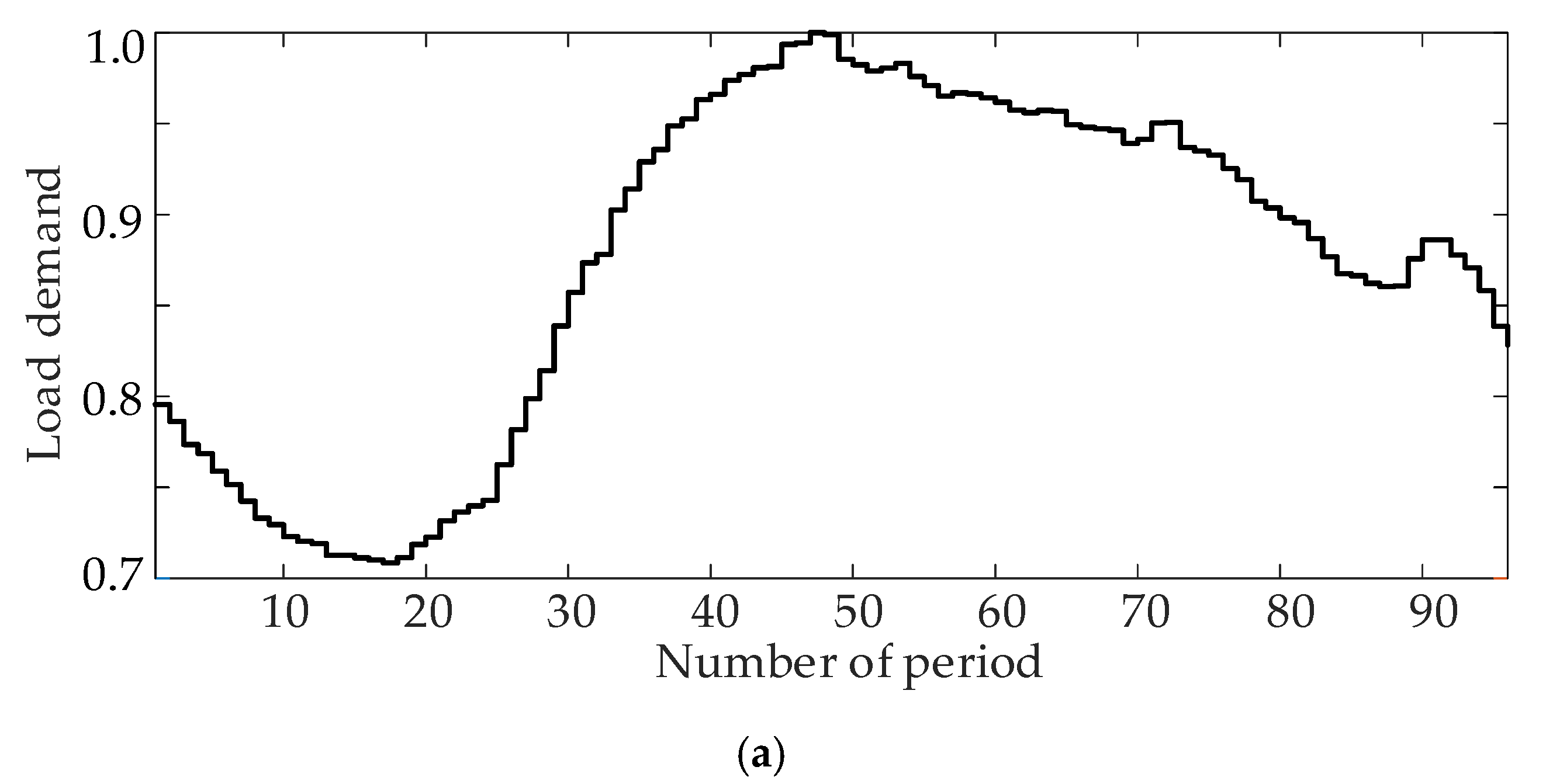
Figure 6a presents the curve of forecast load demand. The original load of the test system is defined as P_load,max, and the ratio of forecasting load at each period to the maximum load is defined as P_load,f/P_load,max. The uncertainties of loads are assumed to be Gaussian distributions with standard deviations of 10% [11,26] of their expected values. Figure 6b shows the curves of the forecast power of four wind farms. In the test system, four wind farms are sufficiently close geographically. Therefore, the forecast outputs of these wind farms have a similar trend. It can be observed that the forecast wind powers show different characteristics compared with the load. The output of wind powers is relatively large at night-time, while the load is opposite. Due to the mismatch of sources and loads, the operating states of the system in different periods need to be analyzed in detail.

4.1.2. Results

The operating state of the test system in each period is assessed using the proposed framework. For the sake of brevity, only the results of some representative periods are presented. The selected periods are 16, 32, 48, 64, 80, and 96. On the one hand, the selected 6 periods cover both day and night. Therefore, various combinations of wind power and load demand can be captured. On the other hand, the extreme scenarios (e.g., maximum generation and minimum load in period 16) can be analyzed to obtain the extreme operating states of the test systems.

The method in Section 2 is adopted to establish the distributions of wind power in each selected period. The distributions of wind power at Bus 14 are shown in Figure 7. It can be found from the results that the probability distributions of wind power output vary with the forecast values. Therefore, it is difficult to find a unified probability distribution that can represent the uncertainties of wind power output in multiple periods. Due to the differences in forecast values, wind power fluctuates in different ranges. For instance, in period 16, wind power has the smallest fluctuation range of [0.574 MW, 0.691MW]. In contrast, wind power has the largest fluctuation range of [0.169 MW, 0.472 MW] in period 48. As mentioned in Section 3.3, the variation of wind power is the critical parameter to determine the number of clusters in the proposed method.

Table 2. The appropriate number of clusters in different periods.

	t = 16	t = 32	t = 48	t = 64	t = 80	t = 96
Number of Clusters	4	8	16	16	16	8

shows the number of clusters determined by the proposed adaptive scheme in each period. It can be seen that the required number of clusters is related to wind power variations. For instance, in periods 16 and 32, the required number of clusters are 4 and 16, respectively. Therefore, when the fluctuation range of wind power is relatively large, more clusters are needed to meet the stopping criterion in (21).

The proposed ACCM is performed to evaluate the operating state of systems in each period. The relative errors and ARMS in (22) and (23) are adopted to verify the accuracy of ACCM. The accuracy of both state and output variables are analyzed, including voltage magnitude, voltage angle, active power, and reactive power. For brevity, only the results of voltage magnitude and active power are presented. Figure 8 presented the results of relative errors. Relative errors provide indicators of the accuracy of expected value μ and standard deviation σ. It can be found from the results that the proposed method could provide the estimation of statistical moments with high accuracy. For voltage magnitude, the maximum errors are observed in period 32. In this case, the mean and maximum relative errors of the expected value of the voltage magnitude are only 0.0018% and 0.0035%, respectively. It is worth to mention that the relative errors in different periods vary in small ranges. The results demonstrate the robustness of the proposed ACCM in evaluating operating states in different periods.

ARMS errors provide an accurate analysis of the distributions of output variables. Figure 9 shows the mean and maximum values of ARMS errors for voltage magnitude and active power. The maximum ARMS errors for voltage magnitude and active power are 0.0999% and 0.0203%, respectively. The results demonstrate that the distributions obtained by the proposed method have minor errors from the results of actual distributions.

The graphical results of voltage magnitude are also presented to demonstrate the effectiveness of ACCM. The probability distributions of voltage magnitude at Bus 18 in periods 16 and 48 are presented in Figure 10; Figure 11, respectively. The results of MCS, TCM, and MCS-LHS [14,15] are adopted to render comparative results. The sample size of MCS is determined by the maximum variance coefficient of output variables, i.e., β_max < 1%. While the trial number of MCS-LHS is selected as 1000 [15]. As it is observed from the results, the proposed ACCM can provide more accurate estimations of probability distributions than TCM and MCS-LHS.

In addition to the expected values and standard deviations of the operating state, the operating risk [36] is also of great concern for the DNOs. Due to the mismatch between DGs output and load demand, risk events such as over/under voltage and overload may occur. Therefore, the probabilistic assessment should provide accurate information to help DNOs underlying the potential risks of the system. In order to verify the efficacy of the proposed ACCM in identifying the risk events, the method was used to determine whether voltage violations occur in periods 16 and 48. In period 16, the wind power output is relatively large, while the load demand is relatively low. Therefore, overvoltage may occur. On the contrary, in period 48, the system is operating at peak load with relatively low wind power, the voltages of buses may fall below the limitations.

The normal operating range of voltage magnitude is assumed as 0.92–1.04 p.u [6]. As shown in Figure 10 and Figure 11, Bus 18 experiences overvoltage in period 16 and undervoltage in period 48. Moreover, the risk values of events are very small, which means that the obtained probability distributions should have high accuracy in the tail regions. ACCM, TCM, MCS-LHS, and MCS are used to calculate the probability of risk, as shown in

Table 3. Risks of voltage violations in different periods.

Methods	t = 16 $\mathbf{Pr}({\mathit{V}}_{18}>1.04\mathbf{p}.\mathbf{u})$	t = 48 $\mathbf{Pr}({\mathit{V}}_{18}<0.92\mathbf{p}.\mathbf{u})$
MCS	0.0027	0.0084
MCS-LHS	0.0011	0.0090
TCM	0.0061	0.0120
ACCM	0.0027	0.0085

. It can be found that TCM and MCS-LHS are less accurate in the tail regions of distributions. In contrast, the results obtained by ACCM have minor errors from the accurate values obtained by MCS. Therefore, the proposed method can help DNOs identify the variables that may endanger the system.

It is worth noting MCS usually requires a large number of samples to obtain the risk of the rare event [35]. For instance, more than 3 × 10⁶ times load flow calculations are required to meet the stopping criterion when calculating the overvoltage risk in period 16. The significant computational burden of MCS hinders its application in a practical system. Compared with MCS-SRS, the proposed ACCM requires fewer load flow calculations to obtain the risk results with reasonable accuracy. Therefore, it has the advantage of high efficiency.

Table 4. The computational burden of different methods.

	MCS	MCS-LHS (1000 Trials)	TCM	ACCM (4 Clusters)	ACCM (8 Clusters)	ACCM (16 Clusters)
Computational time (s)	169.64	4.16	0.87	1.56	2.42	4.18

presents the computational time of each method. MCS is computationally burdensome since it requires a large number of load flow calculations. In contrast, MCS-LHS can significantly reduce the computational burden of MCS due to the adaptation of advanced sampling techniques. The computational time of the proposed ACCM increases with a larger number of clusters. Compared with MCS, the proposed method could achieve the same accuracy with at least 40 times (169/4.18) speed up on efficiency.

4.2. PG&E 69-Bus Case Study

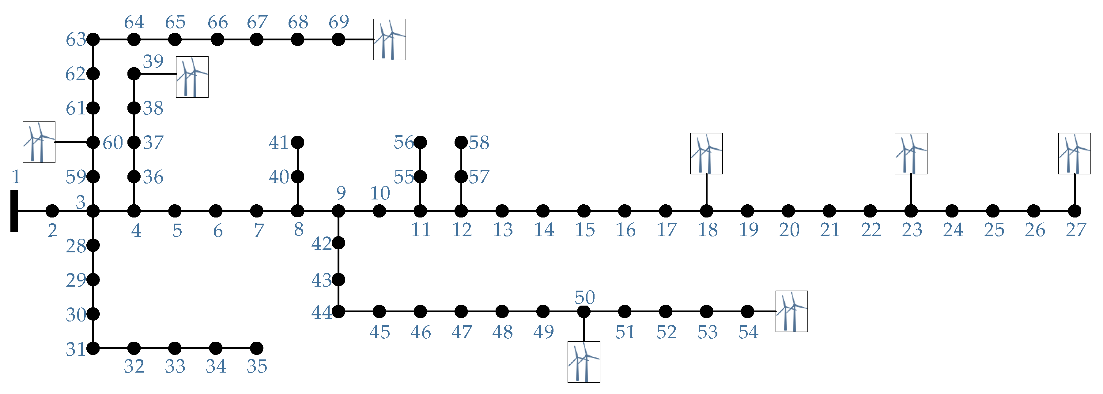
In this section, the performance of the proposed ACCM is analyzed in a relatively large system. Figure 12 presents PG&E 69 bus system with the integration of 8 DGs. For simplicity, only the operating states in period 48 are presented. The original load of the test system [30] is defined as 0.85 P_load,max. The wind farms are integrated into the system at Bus 18, 23, 27, 39, 50, 54, 60, and 69. The nominal power of each wind power is set equally as 0.50 MW. The forecast data of load and wind power are the same as the data in the case studies of the IEEE 33-bus system.

The appropriate number of clusters determined by the adaptive scheme is 8. The accuracy of the proposed method in estimating statistical moments and distributions is analyzed. The results of relative errors and ARMS errors are shown in

Table 5. Relative errors of output variables in period 48.

Relative Error (%)	Mean Values	Max Values
${\epsilon }_{\mu }^{\mathit{V}}$	0.0009	0.0038
${\epsilon }_{\sigma }^{\mathit{V}}$	0.212	1.055
${\epsilon }_{\mu }^{\mathit{\theta }}$	0.164	0.533
${\epsilon }_{\sigma }^{\mathit{\theta }}$	0.382	0.789
${\epsilon }_{\mu }^{\mathit{P}}$	0.102	1.185
${\epsilon }_{\sigma }^{\mathit{P}}$	0.797	3.641
${\epsilon }_{\mu }^{\mathit{Q}}$	0.0974	1.643
${\epsilon }_{\sigma }^{\mathit{Q}}$	0.798	3.638

and

Table 6. ARMS errors of output variables in period 48.

ARMS (%)	Mean	Max
${\mathrm{ARMS}}^{\mathit{V}}$	0.0655	0.695
${\mathrm{ARMS}}^{\mathit{\theta }}$	0.0213	0.231
${\mathrm{ARMS}}^{\mathit{P}}$	0.0182	0.196
${\mathrm{ARMS}}^{\mathit{Q}}$	0.0256	0.271

, respectively. The most significant relative errors of expected values and standard deviations are less than 2% and 4%, respectively. The small values of errors demonstrate the high accuracy of ACCM in estimating statistical moments of output variables. Meanwhile, the excellent performance of ACCM in approximating probability distributions can be validated through the results of ARMS errors.

In period 48, the DGs outputs are relatively low while the load demands are high. Most of the power is supplied through the tie-line between the distribution network and the main grid. Therefore, line 1-2 is the most stressed and may experience the risk of overload. Figure 13 presents he probability distributions of the active power of branch 1-2 are obtained from ACCM and MCS. The results indicate that the distributions obtained by the proposed method close to the reference curve. The performance of the proposed method in fitting the tail of the probability distribution can be verified by calculating rare events. Therefore, we assume that 4 MW is the limitation of the active power of Branch 1-2. Under such circumstances, the risks of overload obtained by the proposed method and MCS are 0.0037 and 0.0039, respectively. The results demonstrate that the proposed ACCM has high accuracy in estimating the tail regions of distributions.

On the comparison of computational burden, the required time of MCS is 197.77s. In contrast, the computational time of ACCM is 3.77s. Compared with the results in Table 4, the computational burden of MCS increased significantly due to the scale of the test system. Since the proposed ACCM only requires a relatively small number of load flow calculations, it can maintain high efficiency in the study of the 69-bus system. Moreover, the efficiency advantage of ACCM can be more notable when applied in large scale systems.

5. Conclusions

This paper proposes a probabilistic framework for the assessment of distribution networks with the integration of DGs. In this framework, the uncertainties of wind power are modeled by using short term forecast values and corresponding forecast errors. Moreover, an adaptive cluster-based cumulant method is proposed for PLF calculation. The performance of the probabilistic framework is evaluated in the IEEE 33-bus system and PG&E 69-bus system. The conclusions are drawn as follows:

• The probability distributions of wind power forecast errors under different forecast values have significant differences in shape and fluctuations. Moreover, the probability distributions of forecast errors provide valuable information for estimating the future operating state of the system.
• The proposed adaptive scheme for determining the number of clusters is related to the variations of wind power. In general, the appropriate number of clusters is increased with the large fluctuations of wind power.
• Due to the significant variations of wind power, the traditional cumulant method fails to obtain accurate tail regions of probability distributions. The proposed adaptive cluster-based cumulant method overcomes this incapability and could achieve high accuracy in estimating statistical moments and distributions with a reasonable computational burden.