Analysis of Inter-Relationships between Urban Decline and Urban Sprawl in City-Regions of South Korea

Abstract

This paper identifies inter-relationships between the urban decline in core areas and urban sprawl in hinterlands using 50 city-regions of South Korea. We measured decline- and sprawl-related indicators and estimated a simultaneous equations model using Three-Stage Least Squares. The results show that population decline and employment decline have a different relationship with urban sprawl. While population decline has a negative impact on the urban sprawl in the density aspect, employment decline worsens the urban sprawl in the morphological aspect. Another result suggests that the difference is related to declining patterns of population and employment. Cities that are experiencing population decline in the core area are likely to lose population in their hinterlands as well. On the other hand, the employment decline in the core area shows a positive correlation with employment growth in hinterlands. The results imply that suburbanization of jobs and the inefficient land use exacerbate the urban sprawl in the morphological aspect. Thus, local governments should pay attention to migration patterns of employment and make multi-jurisdictional efforts. Furthermore, growth management and urban regeneration policies should go hand in hand to tackle this issue.

1. Introduction

Urban decline, generally referring to a phenomenon in which an entire city or part of a city deteriorates over time, has become a major problem in many cities around the world. Demographic and economic declines are generally the causes of this decline. In addition, the decline caused by the outflow of people, businesses, and activities coincides with physical and social decline [1,2,3,4]. There can be a variety of causes behind the urban decline, depending on the circumstances in a city or nation, but the common factors of decline are changes in the macroeconomic conditions and industrial structure. The decline of a core area is highly related to changes in the industrial structure. In particular, many cities, which traditionally grew with their industrial sector, suffer from a decline due to changes in the macro-industrial structure [5].

There are two types of outflows from a core area. The first type takes place when a company moves from a city to another region or country. Globalization has allowed firms to access a large-scale, low-wage workforce in developing countries. This out-of-country movement of firms has led to the loss of traditional jobs, especially in the manufacturing sector, in many towns and cities [6]. The second type of outflow is suburbanization [7,8], occurring when urban areas grow beyond the boundaries of cities commonly with urbanization. Suburbanization also leads to the out-migration of population and economic activities, which can be followed by a subsequent decline of core areas [9]. Demand for new economic activities and associated labor pools is diverted into suburban areas, and it is followed by loss of many jobs in the core areas [4,10]. Moreover, people’s preference for suburban settlements can be one of the causes for this out-migration, considering both dissatisfaction with the current location and attractiveness of a new location [11,12,13,14]. Public policies can also influence that preference. For instance, public policies in the U.S. that promote accessibility and housing affordability in outer areas, such as the construction of expressways and the mortgage system, have led to the suburbanization of certain regions and the decline of central cities [7].

Urban sprawl is one of the types of suburbanization. While there is no internationally agreed-upon definition of urban sprawl, it generally refers to a low-density and unplanned development expanding outward from an urban center [15,16,17]. There are three major characteristics of urban sprawl: the rapid and sporadic spread of low-density, single-family, residential facilities [15], high dependence on private vehicles and the lack of diversity in land use [18], and leapfrogging and linear development patterns [19,20].

In the United States, the housing boom after the Second World War resulted in new patterns of suburban development and soon the term ‘Urban sprawl’ began to be used since the early 1950s [21]. In Western Europe, the concern had already been raised after the First World War; for example, UK first proposed the Metropolitan Green Belt in 1935 in an attempt to prevent urban sprawl [22]. In Eastern Europe, urban sprawl is a relatively recent issue; in Poland, for example, the primary direction of population migration has changed from rural-urban to urban-rural since the 1990s [23]. Similarly, in South Korea, urban sprawl is a recent issue. The country has experienced rapid industrial growth since the 1960–70s and a lot of urban problems due to urban concentration phenomenon have begun to increase. Those problems, such as crime, traffic jams, housing shortage, and pollution, have constantly acted as push factors for migration. Since the 1990–2000s, suburbanization and urban sprawl have become major issues.

Even though various socio-economic forces cause urban sprawl, the most prominent causes are low land prices in the hinterlands and increase in use of private vehicles. Urban sprawl occurs fundamentally when the land price of the hinterlands is lower than that of core areas [24]. In the process of urban growth, competitive housing markets in core areas lead to high land prices. Meanwhile, increasing population densities cause negative externalities, such as traffic congestion and environmental pollution. In contrast, hinterlands have low land prices and healthier environments, which are factors attractive enough to cause out-migration to those areas. The development of automobiles helped to realize this desire to move to the hinterlands. The rapid increase in use of private vehicles has been attributed to the reduction of commuting costs through government investment in transportation infrastructure, such as highways [25]. Furthermore, land use regulations that encouraged low-density development intensified outward diffusion and racial segregation [24,26].

There are both advocates and critics of the impact of urban sprawl. Richardson and Gordon argued that there is a limit to the compact, high-density development in the core areas, and that suburbanization is a better development direction [27]. They emphasized the use of private cars for flexible transportation, safer and less congested traffic, decent public schools, safety from crime, high accessibility to resort and shopping facilities, and low taxation.

Critics, on the other hand, largely focus their arguments on environmental or cost aspects. The environmental impacts of urban sprawl can be categorized into four topics—air, energy, land, and water—and there have been many studies regarding those topics [28]. Soule pointed out urban sprawl’s negative environmental impacts, such as loss of open space, air quality degradation, climate change, water scarcity and quality degradation, and the destruction of wild habitats and ecosystems [29]. Burchell et al. pointed out that sprawl is costly in terms of infrastructure, public administration, real estate development, and traffic [26]. Moreover, urban sprawl acts as a strong pull factor of the out-migration of population and employment from the core area [4,10], which is what we are focusing on in this study. Since suburbs formed by urban sprawl result in cheaper housing and a much more pleasant living environment than that of the central city, they attract people from the central area, which leads to urban decline; accordingly, the declining core area acts as a driving force for urban sprawl [3]. In other words, it is plausible that urban decline and urban sprawl influence each other negatively. This cyclical relationship increases the inefficiency of land use. For example, it hampers the economies of agglomeration in the core area and causes increases in both energy consumption and social costs in the region.

There have been a few empirical studies related to this theory. According to Couch et al., who analyzed urban sprawl in Leipzig and Liverpool, urban decline likely increased the desire for suburban migration [30]. However, the low land prices in declining core areas limited the spread of urban sprawl. Similarly, Downs concluded that the specific characteristics of urban sprawl do not have a significant correlation with urban decline [31]. On the other hand, according to Burchell et al., regression analysis with diverse variables representing urban decline and urban sprawl in 162 U.S. cities showed that various social decline-related variables, such as poverty and crime rates, caused suburban migration [26]. In addition, some of the sprawl-related variables showed a significant effect on urban decline even with weak intensity in the analysis of urban decline as a dependent variable. The results of the study concluded that urban sprawl is largely relevant to the decline. As a result, it can be assumed that a cyclical relationship forms with urban decline mutually influencing urban sprawl. However, the existing empirical studies are limited, and the results also varied. In particular, there have not been many studies about urban sprawl in South Korea where it has not been very long since urban sprawl has become an issue. Nonetheless, since South Korea faces urban decline in core areas alongside urban sprawl in certain regions, a study of the interactions between the two phenomena is necessary.

Given the background, this study seeks to identify the interactions between urban decline and urban sprawl in city regions of South Korea. We aim to find out whether there is a vicious cycle between urban decline and urban sprawl and, if so, which phenomenon has a bigger impact on the other. By clarifying the inter-relationships, we expect to be able to provide policy implications for urban regeneration and growth management at both city and regional levels.

2. Data and Methods

2.1. Flow of Study

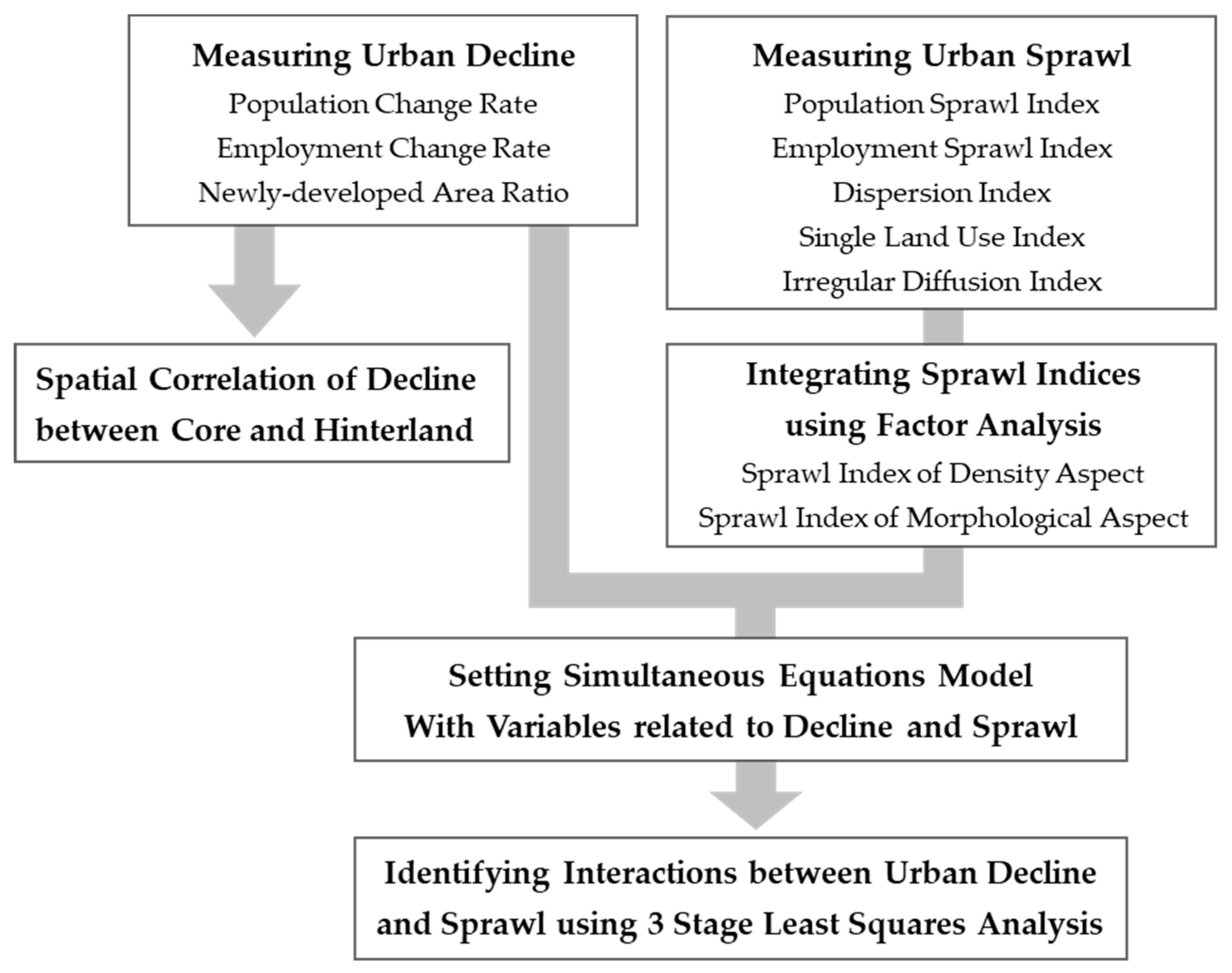
Scheme 1 shows the flow of this study. Urban decline is measured using three indicators. Urban sprawl is measured using five indices; then, the five are integrated into two indices using factor analysis. In order to see if there is a negative spatial interaction, as a preliminary study, correlation analysis between the core area and hinterlands based on the urban decline indicators is conducted. Lastly, the interactions between urban decline and urban sprawl, which is the main objective of this study, are examined using Three-Stage Least Squares analysis.

2.2. Study Area

Although most of the existing studies use a city boundary as a unit of urban sprawl, a better option would be to cover local employment centers and their commuting areas beyond the administrative boundaries of individual cities. Therefore, we use the concept of a Local Labor Market Area (LLMA) as an analysis unit. LLMA is defined as “a geographical unit where most of the interactions between the consumer and the supplier of labor take place” [32]. Since urban sprawl is usually witnessed at a regional level, LLMA can give more meaningful results as a unit of analysis than a single administrative district. We employ the results of Lee [33], which were produced using the 2005 Census data. As shown in Figure 1, the spatial range of this study was 50 LLMAs (except counties), covering the time period from 2000 to 2010. Spatial unit of urban decline is a core area, which was defined as an administrative district housing a city hall and its neighboring districts.

2.3. Measurements of Urban Decline

The decline indicators were selected as shown in

Table 1. Decline Indicators.

Category	Calculation Method
Population Change Rate	Population in a Core Area in 2010/Population in a Core Area in 2000
Employment Change Rate	Number of Employees in a Core Area in 2010/Number of Employees in a Core Area in 2000
Newly-developed Area Ratio	Total Floor Area Developed within 10 Years/Total Floor Area of Developments

. Population and employment changes are typical indicators of decline measures. Newly-developed area ratio is used as a physical decline indicator. Since the word ‘area’ in the ‘newly-developed area’ means ‘floor area’, it includes not only land development, but also re-building or re-modeling on already developed areas. The smaller the values of the three indicators are, the greater the urban decline is.

We see the interaction between urban decline and urban sprawl as a spatial phenomenon between the core area and its hinterland in a city region. The decline of the core area serves as a push factor to drain the population and resources to the hinterland, while the urban sprawl of the hinterland further contributes to the decline of the core area. To verify this hypothesis, we identify population change rate, employment change rate, and newly-developed area ratio of the core area as decline indicators. However, the interaction between urban decline and urban sprawl can vary depending on the pattern of urban decline. Therefore, it will be meaningful to compare the patterns of the decline in the core area and the hinterland as a preliminary analysis. For the analysis, 50 LLMAs are divided into two groups, declining and growing cities, based on population and employment changes in a core area over 10 years. Then, we conducted a correlation analysis of the values of each indicator between the core areas and hinterlands to assess the pattern of decline (or growth).

2.4. Measurements of Urban Sprawl

Urban sprawl involves many characteristics, such as density, shape, and land use. Therefore, it is not easy to quantify. Existing studies on the measurement of urban sprawl can be classified into macroscopic and microscopic analysis methods. Macroscopic methods measure urban sprawl through a single variable, such as population density or employment centrality [34,35,36,37,38,39]. Microscopic methods, on the other hand, employ comprehensive variables that consider various aspects of sprawl. For instance, Ewing and Hamidi calculated the compression-diffusion index of urban areas in the U.S. using density, complex land use, activity centeredness, and road accessibility [40]. Galster et al. analyzed the sprawl index of urban areas in the U.S. using eight indicators: density, continuity, concentration, clustering, centrality, nuclearity, mixed uses, and proximity [41]. Shin and Kim measured urban sprawl in the Seoul metropolitan area in terms of spatial geometry, land use change, population and employment density, and land price distribution [42]. Kotharkar et al. used various indicators reflecting six characteristics of urban sprawl: density, density distribution/dispersion, transportation network, accessibility, shape, and mixed-use land composition [43].

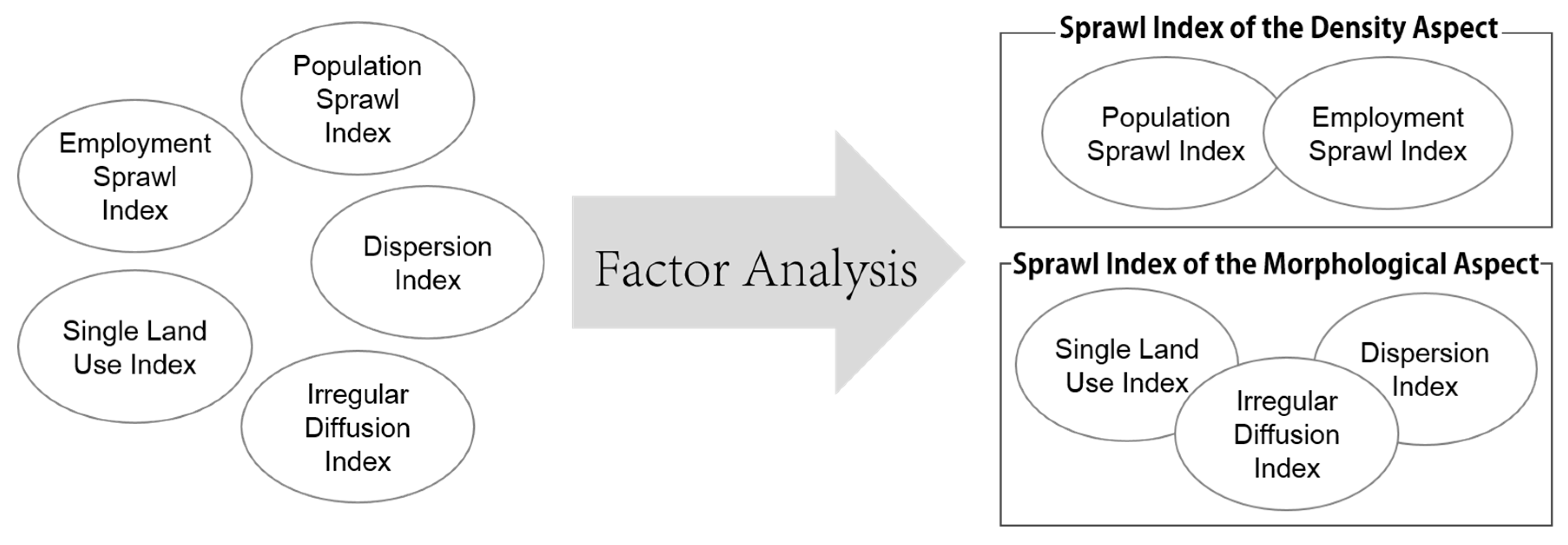
In this study, both the macroscopic and microscopic variables are employed. As shown in Scheme 2, we use the following five indicators that represent the characteristics of urban sprawl: Population sprawl index, Employment sprawl index, Dispersion index, Single land use index, and Irregular diffusion index. After measuring the five indicators, factor analysis is performed to translate them into integrated sprawl indicators, which will be sprawl indices in the density and the morphological aspects.

The first indicator is the population sprawl index, which measures the ratio of change in a city’s urbanized area to population change. Density is the most common and macroscopic variable used in most of the relevant studies for measuring urban sprawl. The following equation is a modified version of Allen et al.’s formula [36].

$${\mathrm{PSI}}_{1-0}=\frac{\left(U{A}_1/U{A}_0\right)}{\left(P_1/P_0\right)}$$

(1)

In Equation (1), PSI_1-0 indicates the population sprawl index of a LLMA during the 2000s; UA₁ indicates the urbanized area of a LLMA in 2010; UA₀ indicates the urbanized area of a LLMA in 2000; P₁ indicates the population in a LLMA in 2010; and P₀ indicates the population in a LLMA in 2000. As the value increases, the degree of sprawl also increases. To calculate urbanized area, we use the land cover map provided by the Ministry of Environment in South Korea.

The second indicator is the employment sprawl index. Like the population sprawl index, it is also an indicator of change in urbanized area over employment change and it uses the total number of workers’ data.

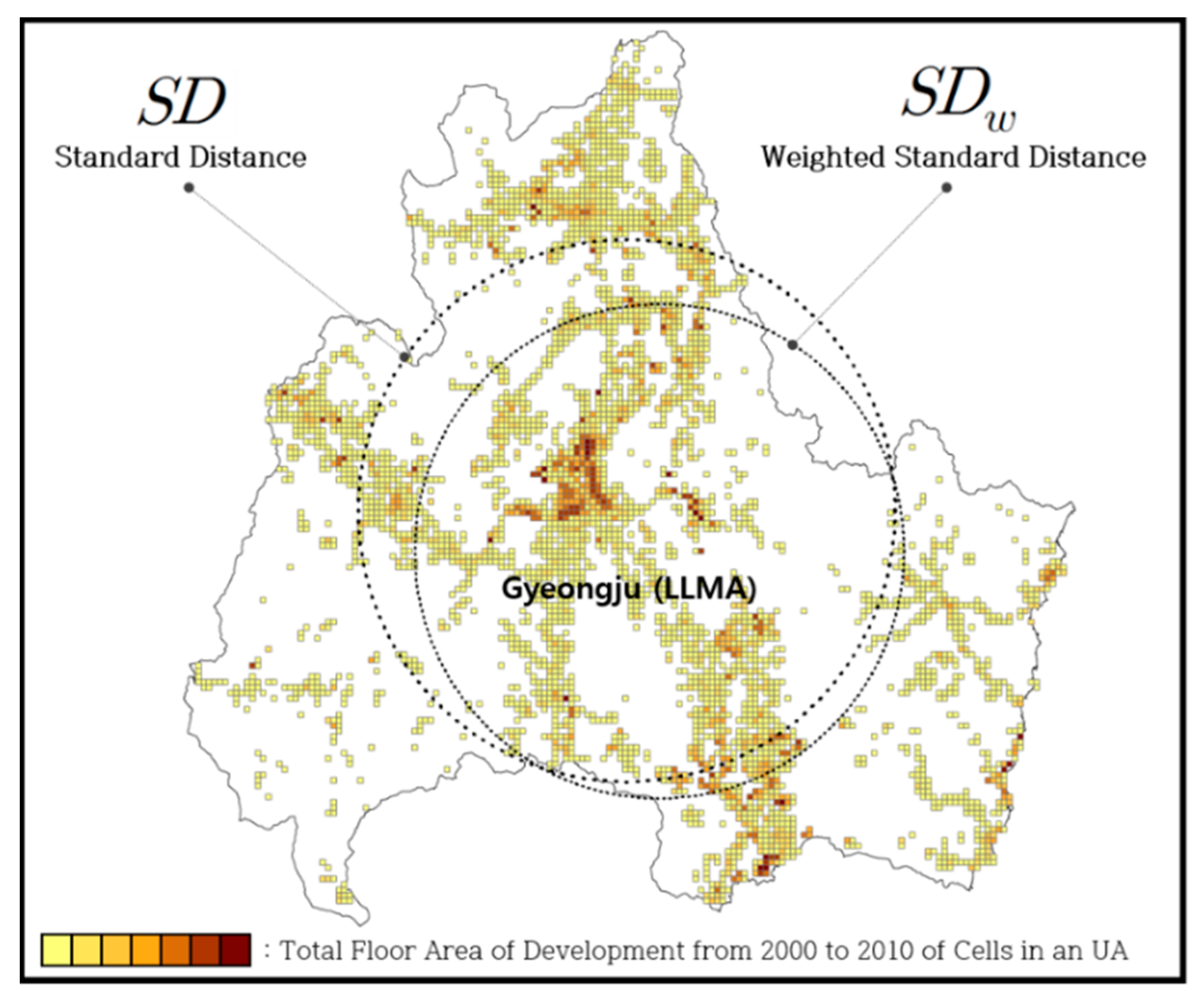
The third indicator is the dispersion index. Even though the aforementioned two indices are useful in determining the degree of sprawl on a macro level, they do not reflect spatial information. Therefore, it is necessary to further analyze micro-level indicators. The dispersion index measures the compactness/dispersion of the development which occurred between 2000 and 2010 in the city regions. This index employs the concept of the standard distance which measures “the degree to which features are concentrated or dispersed around the geometric mean center” [44]. It works the same as the standard deviation in statistics; it gets smaller when the values are closer to the statistical mean.

For this analysis, the urbanized area of each LLMA is divided into 300 m × 300 m grid cells.

$${\mathrm{SD}}_{\mathrm{w}}=\sqrt{\frac{{\sum }_{i=1}^n{w}_i{(x_i-\overline{X_w})}^2}{{\sum }_{i=1}^n{w}_i}+\frac{{\sum }_{i=1}^n{w}_i{(y_i-\overline{Y_w})}^2}{{\sum }_{i=1}^n{w}_i}}$$

(2)

In Equation (2), ($\overline{X_w}$, $\overline{Y_w}$) indicates the x-y coordinates of the weighted mean cell; (x_i, y_i) indicates the x-y coordinates of cell i; and w_i indicates the weight factor of cell i. The dispersion index can be calculated as follows:

$$\mathrm{Dispersion}\mathrm{Index}=\frac{S{D}_w}{SD}$$

(3)

In Equation (3), SD_w is weighted standard distance and SD is unweighted standard distance. The weight in this study is ‘total floor area of development occurred between 2000 and 2010’ in each grid cell; the more development happened near a core area, the smaller the weighted standard distance it gets. In that sense, the unweighted standard distance is like assuming that the city is perfectly evenly developed all over the area between 2000 and 2010. By comparing the weighted standard distance to the unweighted standard distance, we can figure out the centeredness/dispersion of the development that happened between 2000 and 2010 in comparison with a hypothetically and evenly developed situation. The closer the value is to 0, the higher the centrality of development is. 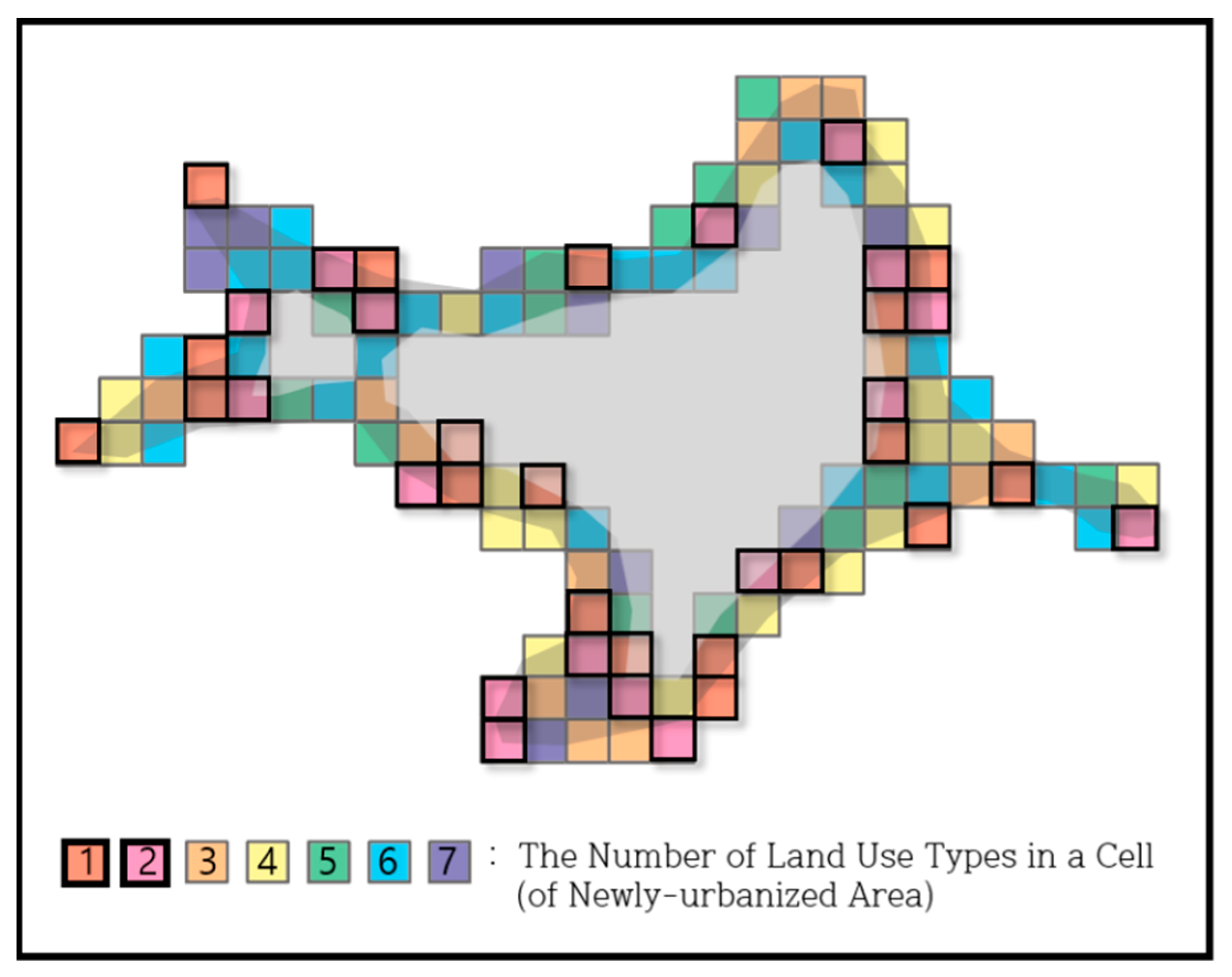Figure 2 illustrates the unweighted and weighted standard distances in the Gyeongju LLMA. The darker the cells are, the more development took place in the cells between 2000 and 2010.The fourth indicator is a single land use index. One of the characteristics of urban sprawl is single land use. If the land use of a city gets monotonous, people need to travel longer distance for a certain activity, which is not an efficient structure. The single land use index calculates the ratio of areas where the number of land use types is one or two. For the calculation, the newly urbanized areas are divided into 1 km × 1 km cells, and the number of land uses is measured for each cell.

$$\mathrm{Sin}\mathrm{gle}\mathrm{Land}\mathrm{Use}\mathrm{Index}=\frac{{\sum }_{m=1}^{k}A{`}_j}{{\sum }_{i=1}^n{A}_i}$$

(4)

In Equation (4), A_i indicates the area of cell i (in a newly urbanized area); A`_j indicates the area of cell j showing monotonous land use; n indicates the number of cells (in a newly urbanized area); and k indicates the number of cells that show monotonous land use. The closer the value is to 1, the more prevalent single land use in the newly urbanized area is. Figure 3 illustrates the concept of this index.

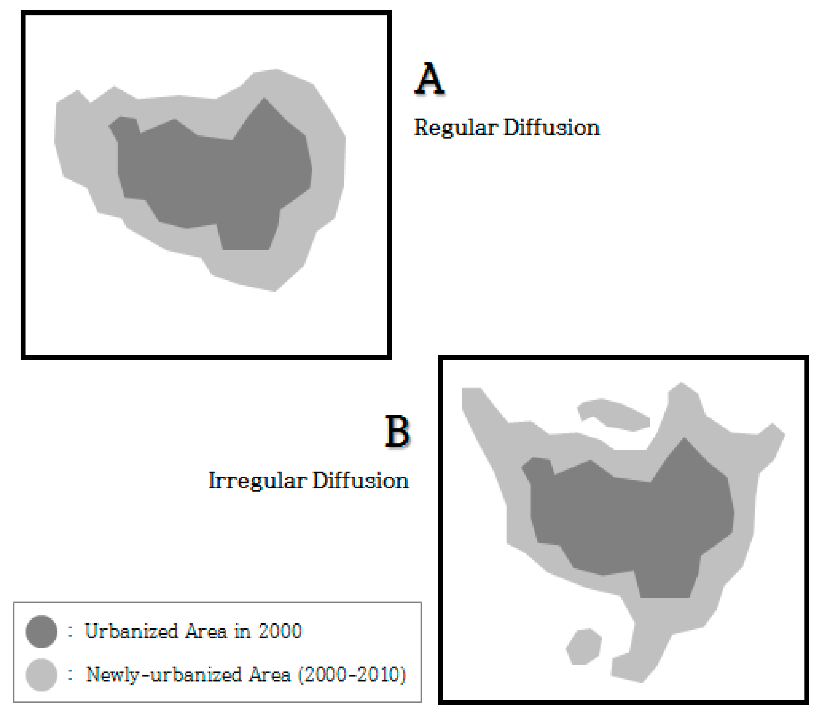
The fifth indicator is the irregular diffusion index. One of the main characteristics of urban sprawl is a linear or irregular spread of development. To measure this development pattern, we utilized the irregular diffusion index of the urbanized area, a numerical measure of the irregularity of the change in the urbanized area between 2000 and 2010 using the urbanized area data.

$$\mathrm{Shape}\mathrm{Index}(\mathrm{SI})=\frac{{P_i}^2}{4\pi A_i}$$

(5)

$$\mathrm{Irregular}\mathrm{Diffusion}\mathrm{Index}=\frac{S{I}_1}{S{I}_0}$$

(6)

The Irregular Diffusion Index indicates the change rate of a Shape Index during a period of time (Equation (6)). The Shape Index measures the irregularity of an urban form based on its perimeter and area [45] and it is designed to have a value of 1 when the shape is a perfect circle. In Equation (5), P_i indicates the perimeter of an urbanized area in LLMA i, and A_i indicates the area of an urbanized area in LLMA i. Figure 4 illustrates the concepts of regular and irregular diffusions based on these indices.

These five indicators are then integrated into two sprawl indices through the factor analysis and are used as endogenous variables in the simultaneous equations model.

2.5. Empirical Model

The simultaneous equations model specifies the inter-relations of urban decline and urban sprawl models as follows:

$$\begin{array}{cc}\hfill PO{P}_{cor{e}_{-}ch}=& {\beta }_0+{\beta }_2\left(EM{P}_{cor{e}_{-}ch}\right)+{\beta }_3\left(ND{R}_{core}\right)+{\beta }_4\left(S{I}_{-}D\right)+{\beta }_5\left(S{I}_{-}M\right)\hfill \\ \hfill & +{\beta }_6\left(PO{P}_{cor{e}_{-}00}\right)+\left[A\right][X_{decline}\left]+\left[\Gamma \right][X_{common}\right]+u\hfill \end{array}$$

(7)

$$\begin{array}{cc}\hfill EM{P}_{cor{e}_{-}ch}=& {{\beta }^{\prime }}_0+{\beta }_1\left(PO{P}_{cor{e}_{-}ch}\right)+{{\beta }^{\prime }}_3\left(ND{R}_{core}\right)+{{\beta }^{\prime }}_4\left(S{I}_{-}D\right)+{{\beta }^{\prime }}_5\left(S{I}_{-}M\right)\hfill \\ \hfill & +{\beta }_7\left(EM{P}_{cor{e}_{-}00}\right)+\left[A^{\prime }\right][X_{decline}\left]+\left[{\Gamma }^{\prime }\right][X_{common}\right]+u^{\prime }\hfill \end{array}$$

(8)

$$\begin{array}{cc}\hfill ND{R}_{core}=& {{\beta }^{″}}_0+{{\beta }^{\prime }}_1\left(PO{P}_{cor{e}_{-}ch}\right)+{{\beta }^{\prime }}_2\left(PO{P}_{cor{e}_{-}ch}\right)+{{\beta }^{″}}_4\left(S{I}_{-}D\right)+{{\beta }^{″}}_5\left(S{I}_{-}M\right)\hfill \\ \hfill & +{\beta }_8\left(DEVDE{N}_{cor{e}_{-}00}\right)+\left[A^{″}\right][X_{decline}\left]+\left[{\Gamma }^{″}\right][X_{common}\right]+u^{″}\hfill \end{array}$$

(9)

$$\begin{array}{cc}\hfill S{I}_D=& {{\beta }^{‴}}_0+{{\beta }^{″}}_1\left(PO{P}_{cor{e}_{-}ch}\right)+{{\beta }^{″}}_2\left(PO{P}_{cor{e}_{-}ch}\right)+{{\beta }^{″}}_3\left(ND{R}_{core}\right)+{{\beta }^{‴}}_5\left(S{I}_{-}M\right)\hfill \\ \hfill & +{\beta }_9\left(POPDE{N}_{cor{e}_{-}00}\right)+\left[B\right][X_{sprawl}\left]+\left[{\Gamma }^{‴}\right][X_{common}\right]+u^{‴}\hfill \end{array}$$

(10)

$$\begin{array}{cc}\hfill S{I}_M=& {{\beta }^{‴\prime }}_0+{{\beta }^{‴}}_1\left(PO{P}_{cor{e}_{-}ch}\right)+{{\beta }^{‴}}_2\left(PO{P}_{cor{e}_{-}ch}\right)+{{\beta }^{‴}}_3\left(ND{R}_{core}\right)+{{\beta }^{‴}}_4\left(S{I}_{-}D\right)\hfill \\ \hfill & +{\beta }_{10}\left(U{A}_{00}\right)+[B^{\prime }][X_{sprawl}\left]+\left[{\Gamma }^{‴\prime }\right][X_{common}\right]+u‴\prime \hfill \end{array}$$

(11)

In Equations (7)–(11), POP_{core_ch}, EMP_{core_ch}, and NDR_core indicate decline-related endogenous variables; SI_D and SI_M indicate sprawl-related endogenous variables; POP_{core_00}, EMP_{core_00}, and DEVDEN_{core_00} indicate lagged variables related to decline; POPDEN_{core_00} and UA₀₀ indicate lagged variables related to sprawl; X_decline, X_sprawl, and X_common, indicate vectors of urban decline factor variables, urban sprawl factor variables, and other control variables, respectively. POP_{core_ch} and EMP_{core_ch} are the population and employment change rates in the core area from 2000 to 2010; NDR_core is the newly-developed area ratio in the core area; SI_D is the sprawl index of the density aspect; and SI_M is the sprawl index in the morphological aspect. The three variables of the urban decline indicator and the two integrated sprawl indices are not independent; rather, they influence each other. Therefore, the dependent variables of each of the five models act as exogenous variables in the other models. Thus, the models are constructed in a way that each contains four different dependent variables as explanatory variables.

Exogenous variables of the simultaneous equations model include lagged variables, control variables, decline factor variables, and sprawl factor variables.

Table A1. Data sources.

Variables		Data Sources
Lagged Variables	population of core area in 2000	Population Census (National Statistical Office)
	number of employees of core area in 2000	Census on Establishments (National Statistical Office)
	development density of core area in 2000	GIS building data (Ministry of Government Administration and Home Affairs)
	population density of core area in 2000	Land Cover Map data (Ministry of Environment)
	urbanized area of LLMA in 2000
Control Variables	aging index in 2000	Population Census
	ratio of highly educated people in 2000
	financial independence rate in 2000	Local Finance Integrated Open System (Ministry of Government Administration and Home Affairs)
	local tax revenue per capita in 2000
	distance from the closest metropolitan city	-
Decline Factor Variables	change rate of the number of businesses with more than 50 employees in the core area	Census on Establishments
	change rate of manufacturing industry in the core area
	change rate of FIRE industry in the core area
	change rate of wholesale and retail industries in the core area
	commercial viability index in the core area
	urban planning tax revenue per capita	Local Finance Integrated Open System
	area of urban regeneration projects	National Statistical Office Ministry of Land, Infrastructure and Transport
	area of housing development projects in the neighboring LLMAs
Sprawl Factor Variables	change rate of Non-Urban Zone
	change rate of Management Zone
	ratio of Management Zone in Non-Urban Zone in 2000
	ratio of Planned Management Zone in Management Zone in 2000
	area of housing development projects
	driving tax per capita in 2000	Local Finance Integrated Open System
	area of industrial complexes	Industrial Complex Statistics (Korea Industrial Complex Corporation)
	area of agro-industrial complexes

in Appendix A describes these variables and their data sources.

The lagged variables are the initial year values associated with each dependent variable, and they act as identification variables for each of them. POP_{core_00}, EMP_{core_00}, DEVDEN_{core_00}, and POPDEN_{core_00} are the population, the number of employees, the development density, and the population density of the core area in 2000, respectively; UA₀₀ is the urbanized area of the LLMA in 2000.

X_common is a vector of control variables, including aging index in 2000, financial independence rate in 2000, ratio of highly educated people in 2000, local tax revenue per capita in 2000, and distance from the closest metropolitan city. Using the ‘distance from the closest metropolitan city’ variable, the effects of proximity to large cities on decline and sprawl are measured. X_decline is a vector of decline factor variables, including change rate of the number of businesses with more than 50 employees in the core area, change rate of the manufacturing industry in the core area, change rate of the FIRE industry in the core area, change rate of the wholesale and retail industries in the core area, commercial viability index in the core area, area of the urban regeneration project, urban planning tax revenue per capita, and area of housing development projects in the neighboring LLMAs. X_sprawl is a vector of sprawl factor variables, including change rate of the Non-Urban Zone, change rate of the Management Zone, ratio of the Management Zone to Non-Urban Zone in 2000, ratio of the Planned Management Zone to Management Zone in 2000, driving tax per capita in 2000, area of housing development projects, area of industrial complexes, and area of agro-industrial complexes. Four of these variables were associated with zoning, which will be helpful to see how urban sprawl was affected by the zoning system and its changes, especially in rural areas.

2.6. Estimation of the Simultaneous Equations Model: Three-Stage Least Squares

Since the simultaneity among the five models noted above causes the endogeneity problem of explanatory variables, bias can occur if the models are estimated separately. Therefore, we use the Three-Stage Least Squares method (3SLS), which is one of the simultaneous equations model’s estimation methods, to solve the problem.

The 3SLS method combines the Two-Stage Least Squares (2SLS) method with the Seemingly Unrelated Regression (SUR) method. The process of estimating the correlation between the error terms in the equation is the same as the SUR method, and the process of solving the endogeneity uses the 2SLS method. Thus, the 3SLS method is asymptotically more effective than the 2SLS method [46]. Using the 3SLS method can resolve the endogeneity between the three decline indicators and the two integrated sprawl indices. This allows for accurate identification of the degree of influence of the interactions.

3. Results

3.1. Measurement of Urban Decline

3.1.1. Results of Measuring Urban Decline in the Core Areas

Table 2. Descriptive Statistics of Decline Indicators.

Variables (n = 50)	Mean	Min.	Max.	Std.D
Population Change Rate	0.96	0.62	1.63	0.19
Employment Change Rate	1.09	0.62	1.63	0.21
Newly-developed Area Ratio	0.22	0.04	0.51	0.21

and

Table 3. Correlation between Decline Indicators.

	Population Change Rate	Employment Change Rate	Newly-Developed Area Ratio
Population Change Rate	1	·	·
Employment Change Rate	0.74 (0.00)	1	·
Newly-developed Area Ratio	0.41 (0.01)	0.42 (0.01)	1

show the results of measuring three decline indicators: population change rate, employment change rate, and newly-developed area ratio.

Population and employment changes showed similar maximum and minimum values, and the regional patterns in Figure 5a,b were similar. On average, the population decreased slightly, while employment increased slightly. On average, 22% of the total development area in the core areas occurred from 2000 to 2010. In the case of development, as shown in Figure 5c, the similarity was not as high as the correlation between population change and employment change, but it showed a positive correlation of 0.4 with both population and employment change rates.

3.1.2. Results of the Correlation Analysis of Urban Decline between Core Areas and Hinterlands

Identifying the spatial correlation of urban decline between core areas and hinterlands can be helpful in understanding the interaction between urban decline and sprawl. In order to see the results of growing and declining regions separately, we divided the 50 LLMAs into two groups based on changes in population and employment in the core area over 10 years.

As shown in

Table 4. Correlation of Urban Decline between Core Areas and Hinterlands in 26 Growing Regions.

	Correlation between Core and Hinterland
Population Change Rate	−0.02 (0.93)
Employment Change Rate	−0.27 (0.18)
Newly-developed Area Ratio	0.03 (0.89)

, the analysis of 26 growing regions showed that growth in population, employment, and development in the core area was not significantly related to the growth or decline in the hinterlands. Meanwhile, decline of the core area in terms of population and employment had a significant correlation with changes in the hinterlands for the 24 declining regions, as shown in

Table 5. Correlation of Urban Decline between Core Areas and Hinterlands in 24 Declining Regions.

	Correlation between Core and Hinterland
Population Change Rate	0.35 (0.09)
Employment Change Rate	−0.50 (0.01)
Newly-developed Area Ratio	−0.12 (0.57)

. Population change in the core area had a positive correlation with the population change in the hinterlands, suggesting that the population decline in the core area was likely to occur together with the population decline in the hinterlands. On the other hand, there was a significant negative correlation between the core area and the hinterlands in the case of employment, which means that employment decline in the core area was likely to occur together with employment growth in the hinterlands. Correlation of the physical changes between the core area and the hinterlands was not statistically significant. In sum, there is no statistical correlation of between core and hinterlands in terms of urban growth or decline. However, in declining regions, the decline of employment in a core area is compensated by the employment gain in suburbs, possibly suggesting that job sprawl affects the economic decline of core areas, and vice versa.

3.2. Measurement of Urban Sprawl

3.2.1. Result of Factor Analysis of Urban Sprawl Indicators

First, as shown in

Table 6. Correlation between Sprawl Indicators.

n = 50	Pop. Sprawl Index	Emp. Sprawl Index	Dispersion Index	Single Land Use Index	Irregular Diffusion Index
Pop. Sprawl Index	1	·	·	·	·
Emp. Sprawl Index	0.90 (0.00)	1	·	·	·
Dispersion Index	0.13 (0.360)	0.02 (0.895)	1	·	·
Single Land Use Index	0.15 (0.317)	0.02 (0.889)	0.33 (0.02)	1	·
Irregular Diffusion Index	0.14 (0.338)	0.04 (0.766)	0.18 (0.22)	0.27 (0.05)	1

, the correlation analysis of the five urban sprawl indicators showed a positive correlation. However, there were large differences in the degree of correlation between variables. The correlation between the population sprawl index and the employment sprawl index was very high, which was an expected result due to the high correlation between population and employment. The other three indicators showed significant correlations in part. The single land use index showed a significant positive correlation with both the dispersion index and the irregular diffusion index. The dispersion index and the irregular diffusion index showed an insignificant, but positive correlation.

Table 7. Factor Analysis Results of Sprawl Indicators (Varimax with Kaiser Normalization).

n = 50	Component
	1	2
Population Sprawl Index	0.966	0.145
Employment Sprawl Index	0.978	−0.023
Dispersion Index	0.027	0.709
Single Land Use Index	0.031	0.779
Irregular Diffusion Index	0.067	0.636

shows the results of the factor analysis, which integrated the five urban sprawl indicators into two dimensions. The first dimension was a sprawl index of the density aspect, which represents an increase in urbanized areas compared to population and employment changes. This was a macroscopic density concept. The other dimension was a sprawl index in the morphological aspect, which reflects the microscopic characteristics of urban sprawl. It includes the other three indicators: dispersion of new development, single land use in newly urbanized areas, and irregular diffusion of urbanized areas. These two integrated sprawl indices are standardized to have values between zero and one and are employed as endogenous variables in the simultaneous equations model.

3.2.2. Results of Measuring Urban Sprawl in the City-Regions

The results of the sprawl index of the density aspect and the sprawl index in the morphological aspect in the 50 LLMAs are shown in

Table 8. Descriptive Statistics of Sprawl Indices.

Variables (n = 50)	Mean	Min.	Max.	Std.D
Sprawl Index in the Density Aspect	0.32	0.00	0.92	0.18
Sprawl Index in the Morphological Aspect	0.53	0.24	0.81	0.15

and Figure 6. The correlation analysis result shown in

Table 9. Correlation between the Two Integrated Sprawl Indices.

	Sprawl Index in the Density Aspect	Sprawl Index in the Morphological Aspect
Sprawl Index in the Density Aspect	1	·
Sprawl Index in the Morphological Aspect	0.34 (0.04)	1

indicates a positive correlation of 0.34 between the two sprawl indices. In Figure 6, not much similarity in spatial patterns between the two indices appeared, which is not that surprising since one of them reflected the density aspect, while the other reflected the shape and land use aspects. This implies that diverse indicators of urban sprawl proposed from literature can be categorized into density and morphological characteristics. An individual sprawl indicator is able to describe the degree of sprawl more precisely for each region. However, the categorization of indicators is useful to diagnose urban sprawl of regions, particularly when many regions are included in the analytical models. The two sprawl variables, sprawl indicators of density and morphological aspects, are employed in the simultaneous equations model as endogenous variables along with three other decline variables, including population and employment change rates and newly-developed area ratio.

3.3. Estimation Results of the Simultaneous Equations Model

3.3.1. Overview

Table 10. Results of the Three-Stage Least Squares Analysis (Structural Equations).

	Models	Population Change Rate		Employment Change Rate		Newly−Developed Area Ratio		Sprawl Index in the Density Aspect		Sprawl Index in the Morpho−Logical Aspect
Variables		Coef.	p	Coef.	p	Coef.	p	Coef.	p	Coef.	p
Intercept		0.164	0.67	0.919 ***	0.00	1.590 ***	0.00	−1.432 ^	0.11	0.276	0.65
Population Change Rate		-	-	0.287 ***	0.01	0.665 ***	0.00	−1.04 ***	0.00	0.707 ***	0.00
Employment Change Rate		0.386 **	0.03	-	-	−0.92 ***	0.01	0.225	0.26	−0.269 *	0.05
Newly−developed Area Ratio		0.019	0.93	−0.122	0.27	-	-	0.218	0.44	0.000	1.00
Sprawl Index in the Density Aspect		−0.046	0.71	−0.044	0.52	−0.089	0.36	-	-	0.249 **	0.03
Sprawl Index in the Morphological Aspect		0.539 ***	0.00	−0.28 ***	0.01	−0.226	0.18	0.869 ***	0.00	-	-
Population of Core Area in 2000		−0.001 ***	0.01	-	-	-	-	-	-	-	-
Number of Employees of Core Area in 2000		-	-	0.000 *	0.09	-	-	-	-	-	-
Development Density of Core Area in 2000		-	-	-	-	−0.07 ***	0.00	-	-	-	-
Population Density of Core Area in 2000		-	-	-	-	-	-	0.018 ***	0.00	-	-
Urbanized Area of LLMA in 2000		-	-	-	-	-	-	-	-	0.000 *	0.09
Aging Index in 2000		0.013	0.94	0.191 **	0.05	0.285	0.08	0.169	0.39	−0.076	0.59
Financial Independence Rate in 2000		0.005 **	0.03	−0.001	0.27	0.001	0.63	0.008 **	0.03	−0.01 ***	0.00
Ratio of Highly Educated People in 2000		0.454	0.51	0.560	0.14	0.252	0.70	−2.108 **	0.01	0.698	0.27
Local Tax Revenue Per Capita in 2000		0.000	0.67	0.000	0.15	0.001 **	0.04	0.001 *	0.09	0.000	0.54
Distance from the Closest Metropolitan City		0.000	0.40	0.000	0.47	0.000	0.83	−0.001 **	0.03	0.000	0.35
Change Rate of the number of Businesses in the Core Area with More than 50 Employees		-	-	0.174 ***	0.00	0.169 **	0.05	-	-	-	-
Change Rate of Manufacturing Industry in the Core Area		-	-	0.942 ***	0.01	−0.087	0.90	-	-	-	-
Change Rate of FIRE Industry in the Core Area		-	-	2.177 ***	0.00	2.574 ***	0.01	-	-	-	-
Change Rate of Wholesale and Retail Industries in the Core Area		1.944 **	0.05	1.721 ***	0.01	2.006 *	0.07	-	-	-	-
Commercial Viability Index in the Core Area		−0.351	0.44	−0.90 ***	0.00	−0.659	0.20	-	-	-	-
Area of Urban Regeneration Projects		0.010	0.18	-	-	0.001	0.75	-	-	-	-
Urban Planning Tax Revenue Per Capita		0.006	0.46	-	-	−0.02 ***	0.01	-	-	-	-
Area of Housing Development Projects in the Neighboring LLMAs		0.000	0.70	0.000	0.37	0.000	0.83	-	-	-	-
Change Rate of Non-Urban Zone		-	-	-	-	-	-	1.494 **	0.03	−0.132	0.79
Change Rate of Management Zone		-	-	-	-	-	-	−0.086	0.57	0.068	0.54
Ratio of Management Zone to Non-Urban Zone in 2000		-	-	-	-	-	-	0.014	0.95	0.217 *	0.08
Ratio of Planned Management Zone to Management Zone in 2000		-	-	-	-	-	-	0.284 ^	0.11	−0.107	0.37
Driving Tax Per Capita in 2000		-	-	-	-	-	-	−0.001	0.90	−0.002	0.64
Area of Housing Development Projects		-	-	-	-	-	-	−0.003	0.18	−0.003	0.12
Area of Industrial Complexes		-	-	-	-	-	-	−0.02 ***	0.00	0.007 **	0.03
Area of Agro-industrial Complexes		-	-	-	-	-	-	−0.096 **	0.03	0.062 *	0.06
System Weighted R−square		0.7888

*** Significant at the 1% level, ** significant at the 5% level, * significant at the 10% level, and ^ significant at the 11% level.

and

Table 11. Interactions between Urban Decline and Urban Sprawl.

	Y	Population Change Rate	Employme-nt Change Rate	Newly-Developed Area Ratio	Sprawl Index in the Density Aspect	Sprawl Index in the Morpho-Logical Aspect
X
Population Change Rate			+	+	-	+
Employment Change Rate		+		-	∙	-
Newly-developed Area Ratio		∙	∙		∙	∙
Sprawl Index in the Density Aspect		∙	∙	∙		+
Sprawl Index in the Morphological Aspect		+	-	∙	+

show the results of the regression estimation of the simultaneous equations model through the 3SLS method. The structural equation coefficients shown in Table 10 are the direct effects of the exogenous variables. The reduced-form equation result is given in Appendix B (

Table A2. Results of the Three-Stage Least Squares Analysis (Reduced-Form Equations).

	Y	Population Change Rate		Employment Change Rate		Newly−Developed Area Ratio		Sprawl Index in the Density Aspect		Sprawl Index in the Morpho−Logical Aspect
X		Coef.	p	Coef.	p	Coef.	p	Coef.	p	Coef.	p
Intercept		0.713	0.35	1.00 ***	0.01	1.258 **	0.02	−1.593	0.19	0.116	0.93
Population of Core Area in 2000		−0.002 ***	0.00	0.000	0.70	−0.001	0.11	0.001	0.28	−0.001 ^	0.10
The Number of Employees of Core Area in 2000		0.000	0.50	0.00 ***	0.00	0.000	0.21	0.000	0.41	0.000	0.77
Development Density of Core Area in 2000		0.000	0.99	0.012	0.40	−0.076 **	0.02	−0.021	0.55	−0.009	0.80
Population Density of Core Area in 2000		0.002	0.74	−0.002	0.40	0.000	0.99	0.022 **	0.02	0.008	0.27
Urbanized Area of LLMA in 2000		0.000	0.25	0.000	0.30	0.000	0.48	0.000	0.32	0.001 ***	0.00
Aging Index in 2000		0.054	0.87	0.202	0.21	0.137	0.57	0.139	0.68	−0.059	0.86
Financial Independence Rate in 2000		0.003	0.53	0.000	0.90	0.004	0.31	0.001	0.77	−0.005	0.38
Ratio of Highly educated People in 2000		1.287	0.37	0.761	0.25	0.453	0.66	−2.480 ^	0.11	0.793	0.59
Local Tax Revenue Per Capita in 2000		0.000	null	0.000	0.55	0.000	null	0.001 ***	0.01	0.000	0.45
Distance from the Closest Metropolitan City		0.000	null	0.000	null	0.000 ^	0.11	−0.001	null	0.000	null
Change Rate of the Number of Businesses in the Core Area with More than 50 Employees		0.072	0.27	0.19 ***	0.00	0.044	0.56	−0.029	0.59	−0.009	0.85
Change Rate of Manufacturing Industry in the Core Area		0.388	0.53	1.234 **	0.04	−0.874	0.28	−0.473	0.46	−0.179	0.76
Change Rate of FIRE Industry in the Core Area		0.894	0.29	2.31 ***	0.00	1.084	0.28	−0.214	0.76	−0.052	0.94
Change Rate of Wholesale and Retail Industries in the Core Area		3.830 **	0.01	2.06 ***	0.01	2.359 **	0.04	−1.434	0.24	1.809	0.13
Commercial Viability Index in the Core Area		−0.910	0.33	−1.09 **	0.02	−0.255	0.72	0.436	0.38	−0.243	0.67
Area of Urban Regeneration Projects		0.015	0.28	0.001	0.79	0.009	0.38	−0.006	0.49	0.009	0.33
Urban Planning Tax Revenue Per Capita		0.010	0.53	0.004	0.31	−0.014	0.27	−0.009	0.39	0.004	0.76
Area of Housing Development Projects in the Neighboring LLMAs		0.000	0.85	0.001	0.12	−0.001	0.60	0.000	0.95	0.000	0.72
Change Rate of Non−Urban Zone		0.067	0.91	−0.157	0.58	−0.051	0.89	1.729 *	0.10	0.385	0.72
Change Rate of Management Zone		0.047	0.70	−0.014	0.80	0.027	0.68	−0.048	0.84	0.093	0.72
Ratio of Management Zone to Non−Urban Zone in 2000		0.180	0.38	−0.083	0.39	0.086	0.54	0.190	0.52	0.414	0.20
Ratio of Planned Management Zone to Management Zone in 2000		−0.053	0.70	0.000	1.00	−0.041	0.59	0.263	0.33	−0.077	0.78
Driving Tax Per Capita in 2000		−0.002	0.68	0.001	0.66	−0.001	0.73	−0.003	0.77	−0.005	0.65
Area of Housing Development Projects		−0.003	0.40	0.002	0.33	−0.001	0.62	−0.006	0.12	−0.007	0.12
Area of Industrial Complexes		0.004	0.40	0.000	0.88	0.003	0.36	−0.014 **	0.03	0.006	0.40
Area of Agro-industrial Complexes		0.041	0.35	−0.010	0.62	0.025	0.37	−0.068	0.36	0.078	0.32

*** Significant at the 1% level, ** significant at the 5% level, * significant at the 10% level, and ^ significant at the 11% level.

), which indicates that the number of significant variables are significantly less than the results of the structural equations, but the signs are mostly consistent. Table 11 summarizes, from Table 10, the interactions between decline and sprawl-related variables; plus (blue) signs mean positive impacts, minus (red) signs mean negative impacts, and dots mean insignificant impacts. It should be noted that the smaller the values of the decline-related variables are, the more the city is declined. Thus, minus signs in Table 11 implies a vicious circle between urban decline and urban sprawl.

3.3.2. Results of the Models

The first three columns in Table 10 are the results of urban decline models: population change rate, employment change rate, and newly-developed area ratio. Below are major findings from the significant variables on those models. First, the ‘population’ and ‘development density’ of the core area in the initial year were significantly negative. It indicates that the rate of change tends to increase as the population and development in the initial year were smaller. On the other hand, ‘employment’ of the core area in the initial year was significantly positive, which indicates that there was more employment growth afterward in the region where the size of total employment was already large in the initial year.

The control variables of aging index, financial independence rate, ratio of highly educated people, local tax revenue per capita in the initial year, and the distance from the closest metropolitan city have partially significant effects depending on the models. The aging index in the first year shows significant positive effects on the employment and development changes in the core area, the financial independence rate on the population change, and the local tax revenue per capita on the developmental change.

As a factor variable of urban decline, the change rate of the number of businesses with 50 or more employees in the core area has a positive effect on the employment change rate and the newly-developed area ratio in the core area. In addition, changes in manufacturing, FIRE, and the wholesale and retail industries in the core area have partially significant positive effects on urban decline. On the other hand, the commercial viability index in the core area turns out that it has a negative impact on employment change in the core area. Lastly, the urban planning tax revenue per capita in the initial year shows a negative impact on the newly-developed area ratio in the core area, which implies that it has promoted more planned development.

The latter two columns in Table 10 are the results of urban sprawl models: sprawl index in the density aspect and the morphological aspect.

The variables that affect sprawl-related dependent variables are as follows. The population density of the core area and the urbanized area of the LLMA in the initial year are significantly positive. In other words, a higher population density of the core area and a larger urbanized area in the initial year indicates a more negative occurrence of sprawl.

Among the control variables, the financial independence rate, ratio of highly educated people, local tax revenue per capita in the initial year, and the distance from the closest metropolitan city have a significant effect on urban sprawl. The distance from the closest metropolitan city was negative, suggesting that urban sprawl was more likely to happen in the region close to large cities.

Among the factor variables of urban sprawl, four of them are related to zoning and three of those variables show a statistically significant and positive value. The change rate of the Non-Urban Zone has a significantly positive impact on the sprawl in the density aspect. This correlation is presumably due to the fact that high-density development often occurs with converting the Non-Urban Zone into an Urban Zone. The ratio of the Management Zone to the Non-Urban Zone in the initial year shows a significantly positive effect on the sprawl in the morphological aspect. Considering that Management Zone is available for development, a large proportion of the Management Zone can cause a more unfavorable form of unplanned development.

The interaction between urban decline and urban sprawl, which is the main focus of this study, is somewhat complicated. First, it indicates that population decline in the core area exacerbates the sprawl in the density aspect (−1.04) as expected, while the effect of the urban sprawl on population decline in the core area (−0.046) is not statistically significant. However, there are two facts that need to be considered together in interpreting this result. One is that a population change in a core area is not largely related to a change of urbanized area in the entire LLMA, as shown in the

Table A3. T-test result of ‘changes in urbanized area’ between two groups: LLMAs whose ‘core’ experienced population decline and LLMAs whose ‘core’ experienced population growth.

Group	Mean	p-Value
LLMAs whose ‘core’ experienced population decline	1.237	0.470
LLMAs whose ‘core’ experienced population growth	1.242

and

Table A4. T-test result of ‘changes in urbanized area’ between two groups: LLMAs whose ‘hinterland’ experienced population decline and LLMAs whose ‘hinterland’ experienced population growth.

Group	Mean	p-Value
LLMAs whose ‘hinterland’ experienced population decline	1.185	0.028
LLMAs whose ‘hinterland’ experienced population growth	1.319

. The other fact is that the population decline in the core area was likely to occur along with the population decline in the hinterland, as shown in the Table 5. All things considered, we can infer that the increase of sprawl index in the density aspect may be affected substantially by the population decrease in the whole city-region, not necessarily by the decrease in the core area. On the other hand, the sprawl index in the morphological aspect is shown to be reduced by the decreasing population in the core areas, and vice versa. That means, as population decreases in the core area, urbanization occurs in rather regular and desirable forms. In summary, a decreasing population does have a significant impact on sprawl index in the density aspect, but there is no cyclical interaction between the two phenomena since population in the core area and the hinterland decrease together. In addition, population decrease in a core area is shown to mitigate the urban sprawl in the morphological aspect.

Second, the employment decline in the core area had no significant impact on the sprawl index in the density aspect, and vice versa. However, the employment decline is shown to exacerbate the sprawl index in the morphological aspect, and vice versa. The reason for the different results from the population decline seems to be the difference in the decline patterns between population and employment. In the case of population decline in the core area, the sprawl index in the density aspect was high due to the overall decrease in population throughout the region. On the other hand, the decline in employment in the core area had a positive correlation with the employment growth in the hinterland, as shown in Table 5. In other words, the decline in employment in the core area was likely to occur along with the suburbanization of employment, which made the employment density in the whole region relatively constant. Therefore, even though suburbanization of employment occurring in the process of employment decline in the core area could not be seen as urban sprawl in the density aspect, this phenomenon can be called urban sprawl because negative forms of development took place in this process, and those development patterns, in return, exacerbate employment decline in the core area.

4. Discussions

While many cities have been experiencing urban decline in recent years, urban sprawl is also a major issue. Suburbanization inevitably happens during the process of urban growth, but suburbanization in a declining city can cause negative consequences. One major consequence is being ended up with inefficient land use in both the core areas and hinterlands. In this study, we tried to clarify the interaction between the two negative phenomena occurring in the center and periphery of the city. For this purpose, we specified and measured urban decline and sprawl indicators for city-regions and estimated their inter-relationships through a simultaneous equations model. From the analysis, we made three major findings.

First, there are positive correlations between the decline-related variables: population change rate, employment change rate, and newly-developed area ratio. However, the results of the correlation analysis of decline variables between the core area and its hinterland were different among variables; population in the core area showed a tendency to decline, together with its hinterland, while the employment in the core area and hinterland changed in an opposite way.

Second, five sprawl-related indicators were integrated into two dimensions. One was a sprawl index in the density aspect, which combined the population sprawl index and employment sprawl index. The other was the sprawl index in the morphological aspect that combined the dispersion index, single land use index, and irregular diffusion index, and contained microscopic characteristics, such as land use and urbanization patterns. While many studies use diverse indicators to examine urban sprawl for specific case study areas, they may generate different results depending on what indicators are employed because each indicator is measured by different variables, such as population, employment, land use, and so on, and spatial units, such as grid, city, and region. By and large, the categorized sprawl indicators, density and morphological aspects, can capture such diversity and diagnose large samples of regions when utilized in an econometric model.

Thirdly, the results of the 3SLS analysis showed that the declines in population and employment differed in their interactions with urban sprawl. Population decline in the core area increased the sprawl index in the density aspect, but decreased the sprawl index in the morphological aspect. Given that population decline in a core area is likely to occur together with decline in the surrounding area, it seems to be the result of consecutive or inward urbanization in the process of population decline and, thus, it is hard to say that there is an interaction between population decline in a core area and urban sprawl in the surrounding area. On the other hand, although it does not have a significant effect on the sprawl index in the density aspect, the employment decline is negatively correlated with the sprawl index in the morphological aspect. They both have a significant negative impact on each other. Considering the fact that the employment decline in the core area had a significantly negative correlation (−0.5) with the employment decline in the surrounding area, it is plausible to say that there is a negative inter-relationship between employment decline in the core area and an undesirable form of development in the hinterlands; the suburbanization of jobs causes an inefficient development in the outskirts and then the new jobs attract more employment from the core area and accelerate the decline in the area. This is more noticeable for declining regions rather than growing regions as discussed in Section 3.1.

In conclusion, this study suggests that “job sprawl” is a potential main culprit of the negative inter-relationship between a core area and hinterlands in a city-region. Intra-urban decentralization of jobs causes an inefficient form of land use in the suburbs and weakens the competitiveness and attractiveness of the core area, which further stimulates more jobs to move out of the core area. On the other hand, population did not migrate in the same way as employment does; the population in the core area increases or decreases together with the population in the hinterland.

In the case of South Korea, therefore, employment is an important key in planning the sustainable urban spatial structure. This is an intriguing result since it is not what many researchers have discussed. Existing studies on the interaction between urban decline and sprawl have mostly focused on residential and population migration issues [26,31]; living environment elements, such as housing prices, school level, crime rates, traffic jams, and air pollution, are the main reasons that make suburbs a more attractive option [47], and their relocation to the suburbs will make the core area more deteriorated. Moreover, studies on job sprawl are largely focusing on the spatial mismatch issue and the resultant inefficiency in land use and transportation [48,49,50]. No studies imply that job sprawl can be such a crucial factor that creates a negative cycle with the deterioration of urban center. However, the result of this study indicates that the migration of employment can possibly play a key role in the interaction between urban decline and sprawl. Therefore, policymakers should pay close attention to the migration patterns of employment in city-regions.

In addition, macro-level growth management policy and micro-level urban regeneration policy should be linked together to tackle both the problems of urban decline and sprawl. One fundamental reality is that all kinds of growth or decline-related problems are regional, not local. Thus, individual localities cannot effectually cope with these problems; they should put multi-jurisdictional efforts within the region.

References

1. Cheshire, P.C.; Dennis, G.H. Urban Problems in Western Europe: An Economic Analysis; Hyman: London, UK, 1989; ISBN 9780044450108. [Google Scholar]
2. Beauregard, R.A. Representing urban decline: Postwar cities as narrative objects. Urban Aff. Q. 1993, 29, 187–202. [Google Scholar] [CrossRef]
3. Wagner, F.W.; Joder, T.E.; Mumphrey, A.J., Jr.; Akundi, K.M.; Artibise, F.J. Revitalizing the City: Strategies to Contain Sprawl and Revive the Core; M.E. Sharpe, Inc: New York, NY, USA, 2005; ISBN 9780765612434. [Google Scholar]
4. Roberts, P.; Sykes, H. Urban Regeneration: A Handbook; SAGE Publications Ltd.: London, UK, 2000; ISBN 9780761967170. [Google Scholar]
5. Fraser, C. Change in the European industrial city. In Urban Regeneration in Europe; Couch, C., Charles, F., Susan, P., Eds.; Blackwell Science Ltd.: Oxford, UK, 2003; pp. 17–33. ISBN 9780632058419. [Google Scholar]
6. Scott, A.J. Flexible production systems and regional development: The rise of new industrial spaces in North America and Western Europe. Int. J. Urban Reg. 1988, 12, 171–186. [Google Scholar] [CrossRef]
7. Bradbury, K.L.; Anthony, D.; Kenneth, A.S. Urban Decline and the Future of American Cities; Brookings Institution Press: Washington, DC, USA, 1982; ISBN 9780802832689. [Google Scholar]
8. Gainsborough, J.F. Slow growth and urban sprawl: Support for a new regional agenda? Urban Aff. Rev. 2002, 37, 728–744. [Google Scholar] [CrossRef]
9. Downs, A. New Visions for Metropolitan America; Brookings Institution Press: Washington, DC, USA, 1994; ISBN 9780815719250. [Google Scholar]
10. Kasarda, J.D. Industrial restructuring and the changing location of jobs. In State of the Union: America in the 1990s, Volume 1: Economic Trends; Farley, R., Ed.; Russell Sage Foundation: New York, NY, USA, 1995; pp. 215–268. ISBN 9780871542403. [Google Scholar]
11. Yi, C.; Kim, K. A machine learning approach to the residential relocation distance of households in the Seoul metropolitan region. Sustainability 2018, 10, 2996. [Google Scholar] [CrossRef] [Green Version]
12. Moore, E.G. Residential Mobility in the City; Association of American Geographers: Washington, DC, USA, 1972. [Google Scholar]
13. Loren, D.L.; Eva, K.; Boaz, K. Residential relocation of amenity migrants to Florida: “Unpacking” post-amenity moves. J. Aging Health 2010, 22, 1001–1028. [Google Scholar]
14. Lee, B.H.Y.; Paul, W. Residential mobility and location choice: A nested logit model with sampling of alternatives. Transportation (Amst.) 2010, 37, 587–601. [Google Scholar] [CrossRef] [Green Version]
15. Burchell, R.W.; Naveed, A.S.; David, L.; Hilary, P.; Anthony, D.; Samuel, S.; Judy, S.D.; Terry, M.; David, H.; Michelle, G. The Costs of Sprawl–-Revisited; Transportation Research Board: Washington, DC, USA, 1998; ISBN 9780309063067. [Google Scholar]
16. DeSalvo, J.S.; Su, Q. The determinants of urban sprawl: Theory and estimation. Int. J. Urban Sci. 2019, 23, 88–104. [Google Scholar] [CrossRef]
17. Woo, M.; Guldmann, J.M. Impacts of urban containment policies on the spatial structure of US metropolitan areas. Urban Stud. 2011, 48, 3511–3536. [Google Scholar] [CrossRef]
18. Song, Y.; Knaap, J. Measuring urban form: Is Portland winning the war on sprawl? J. Am. Plan. Assoc. 2004, 70, 210–225. [Google Scholar] [CrossRef]
19. Torrens, P.; Alberti, M. Measuring Sprawl. Working Paper Series of Centre for Advanced Spatial Analysis; University College: London, UK, 2000; pp. 1–43. [Google Scholar]
20. Tsai, Y.H. Quantifying urban form: Compactness versus ‘sprawl’. Urban Stud. 2005, 42, 141–161. [Google Scholar] [CrossRef]
21. Laas, W. The Suburbs are Strangling the City. New York Times Magazine, 18 June 1950. [Google Scholar]
22. Thomas, D. London’s green belt: The evolution of an idea. Geogr. J. 1963, 129, 14–24. [Google Scholar] [CrossRef]
23. Raźniak, P.; Winiarczyk-Raźniak, A. Influence of the societal security level on population migrations in Poland. Procedia-Soc. Behav. Sci. 2014, 120, 2–12. [Google Scholar] [CrossRef] [Green Version]
24. Pendall, R. Do land-use controls cause sprawl? Environ. Plan. B 1999, 26, 555–571. [Google Scholar] [CrossRef]
25. Brueckner, J.K. Urban sprawl: Diagnosis and remedies. Int. Reg. Sci. Rev. 2000, 23, 160–171. [Google Scholar] [CrossRef]
26. Burchell, R.W.; George, L.; William, R.D.; Catherine, C.G.; Anthony, D.; Samuel, S.; Katherine, G.S.; Terry, M. Costs of Sprawl-2000; Transportation Research Board: Washington, DC, USA, 2002; ISBN 9780309067195. [Google Scholar]
27. Richardson, H.W.; Peter, G. Compactness or sprawl: America’s future vs. the present. In Cities for the New Millennium; Echenique, M., Saint, A., Eds.; SPON Press: London, UK, 2001; pp. 53–64. [Google Scholar]
28. Wilson, B.; Chakraborty, A. The environmental impacts of sprawl: Emergent themes from the past decade of planning research. Sustainability 2013, 5, 3302–3327. [Google Scholar] [CrossRef] [Green Version]
29. Soule, D.C. Urban Sprawl: A Comprehensive Reference Guide; Greenwood Press: Westport, CT, USA, 2006; ISBN 9780313320385. [Google Scholar]
30. Couch, C.; Karecha, J.; Nuissl, H.; Rink, D. Decline and sprawl: An evolving type of urban development–observed in Liverpool and Leipzig 1. Eur. Plan. Stud. 2005, 13, 117–136. [Google Scholar] [CrossRef]
31. Downs, A. Some realities about sprawl and urban decline. Hous. Policy Debate 1999, 10, 955–974. [Google Scholar] [CrossRef]
32. Casado-Díaz, J.M. Local Labour Market Areas in Spain: A Case Study. Reg. Stud. 2000, 34, 843–856. [Google Scholar] [CrossRef]
33. Lee, S. A study on the measurement and applicability of Local Labour Market Areas (LLMAs) in Korea. Q. J. Labor Policy 2008, 8, 147–182. [Google Scholar]
34. Fulton, W.B.; Pendall, R.; Nguyen, M.; Harrison, A. Who Sprawls Most? How Growth Patterns Differ Across the US; Brookings Institution, Center on Urban and Metropolitan Policy: Washington, DC, USA, 2001. [Google Scholar]
35. Kahn, M.E. Does sprawl reduce the Black/White housing consumption gap? Hous. Policy Debate 2001, 12, 77–86. [Google Scholar] [CrossRef]
36. Allen, J.; Kang, L. Modeling and prediction of future urban growth in the Charleston region of South Carolina: A GIS-based integrated approach. Conserv. Ecol. 2003, 8, 1–20. [Google Scholar] [CrossRef] [Green Version]
37. Lopez, R.; Hynes, H.P. Sprawl in the 1990s: Measurement, distribution and trends. Urban Aff. Rev. 2003, 38, 325–355. [Google Scholar] [CrossRef] [PubMed]
38. Zitti, M.; Ferrera, C.; Perini, L.; Carlucci, M.; Salvati, L. Long-term urban growth and land use efficiency in Southern Europe: Implications for sustainable land management. Sustainability 2015, 7, 3359–3385. [Google Scholar] [CrossRef] [Green Version]
39. Liu, L.; Peng, Z.; Wu, H.; Jiao, H.; Yu, Y.; Zhao, J. Fast identification of urban sprawl based on K-means clustering with population density and local spatial entropy. Sustainability 2018, 10, 2683. [Google Scholar] [CrossRef] [Green Version]
40. Ewing, R.; Hamidi, S. Measuring Urban Sprawl and Validating Sprawl Measures; National Institutes of Health and Smart Growth America: Washington, DC, USA, 2014.
41. Galster, G.; Hanson, R.; Ratcliffe, M.R.; Wolman, H.; Coleman, S.; Freihage, J. Wrestling sprawl to the ground: Defining and measuring an elusive concept. Hous. Policy Debate 2001, 12, 681–717. [Google Scholar] [CrossRef]
42. Shin, J.; Kim, J. Reappraisal of the issues on the urban sprawl and the urban sprawl measurement based on spatial analysis methodology. Seoul Law Rev. 2012, 19, 317–354. [Google Scholar]
43. Kotharkar, R.; Bahadure, P.; Sarda, N. Measuring compact urban form: A case of Nagpur City, India. Sustainability 2014, 6, 4246–4272. [Google Scholar] [CrossRef] [Green Version]
44. Standard Distance. Available online: https://desktop.arcgis.com/en/arcmap/10.3/tools/spatial-statistics-toolbox/standard-distance.htm (accessed on 25 January 2020).
45. Frenkel, A.; Ashkenazi, M. Measuring urban sprawl: How can we deal with it? Environ. Plan. B 2008, 35, 56–79. [Google Scholar] [CrossRef] [Green Version]
46. Henningsen, A.; Hamann, J.D. Systemfit: A package for estimating systems of simultaneous equations in R. J. Stat. Softw. 2007, 23, 1–40. [Google Scholar] [CrossRef] [Green Version]
47. Woo, M.; Guldmann, J.-M. Urban containment policies and urban growth. Int. J. Urban Sci. 2014, 18, 309–326. [Google Scholar] [CrossRef]
48. Terplan, E.; Jun, S.; Miller, L.; Yilmaz, B. Job Sprawl in the Megaregion; Policy Paper Library, San Francisco Planning and Urban Research Association: San Francisco, CA, USA, 2009. [Google Scholar]
49. Jaret, C.; Adelman, R.M.; Reid, L.W. Suburban sprawl, racial segregation, and spatial mismatch in metropolitan America. Sociation Today 2006, 4, 1–38. [Google Scholar]
50. Stoll, M.A. Job sprawl, spatial mismatch, and black employment disadvantage. J. Policy Anal. Manag. 2006, 25, 827–854. [Google Scholar] [CrossRef] [Green Version]
Scheme 1. Research Flow.
Sustainability 12 01656 sch001
Figure 1. Local Labor Market Areas and Their Core Areas in South Korea.
Sustainability 12 01656 g001
Scheme 2. Measurements of urban sprawl in two aspects.
Sustainability 12 01656 sch002
Figure 2. Standard Distance and Weighted Standard Distance in the Gyeongju LLMA.
Sustainability 12 01656 g002
Figure 3. Diagram of the Concept of Single Land Use Index.
Sustainability 12 01656 g003
Figure 4. Diagram of Regular Diffusion and Irregular Diffusion.
Sustainability 12 01656 g004
Figure 5. Spatial distribution of the population decline (a), employment decline (b), and physical decline (c).
Sustainability 12 01656 g005
Figure 6. Spatial distribution of the sprawl index in the density aspect (a) and the morphological aspect (b).
Sustainability 12 01656 g006