Article

Spatial Analysis of Socio-Economic Driving Factors of Food Expenditure Variation between Provinces in Indonesia

1
Department of Agricultural Economics and Management, Northeast Forestry University, Harbin 150040, Heilongjiang, China
2
Center for Regional Systems Analysis, Planning and Development (CRESTPENT/P4W), IPB University, Bogor 16144, Indonesia
3
Research Center for Plant Conservation and Botanic Gardens, Indonesian Institute of Sciences, Bogor 16003, Indonesia
*
Author to whom correspondence should be addressed.
Sustainability 2020, 12(4), 1638; https://doi.org/10.3390/su12041638
Submission received: 13 January 2020 / Revised: 8 February 2020 / Accepted: 13 February 2020 / Published: 21 February 2020

Abstract

:
Food security has become one of the global challenges; therefore, monitoring food consumption is required. As food consumption is a resultant of food availability at an affordable price, food expenditure actually is a key indicator to assess food security policy. Particularly, the link of food expenditure with socio-economic factors based on the perspective of spatial connectivity should be understood as nowadays food supply and demand between regions are increasingly connected. This study aims to define socio-economic driving factors of food expenditure that considering spatial connectivity between provinces in Indonesia. Data of household food expenditure and socio-economic factors by province including urbanization level, economic growth, gross domestic regional product (GDRP) per capita, poverty severity index, and unemployment rate were used. The preliminary test on the spatial correlation of food expenditure showed a significant result; thus, a spatial regression approach was employed. The results showed that declining food expenditure did not simply indicate increasing prosperity. Larger income disparity among the poor has become crucial to detect lower food expenditure caused by a lack of income. In addition, the increasing unemployment rate was followed by increasing food expenditure. Despite economic growth, increasing GDRP per capita and urbanization contributing to declining food expenditure, both poverty and unemployment are the main issues that threaten household’s ability to afford food. Furthermore, the effect of food expenditure in the neighboring region is also significant, but it shows a contradictory relationship as food expenditure in a region is decreasing when food expenditure in its neighbors is increasing, and vice versa. Therefore, reducing disparities in economic growth, GDRP per capita, urbanization, poverty, and unemployment rate between provinces is also crucial to support more equal food expenditure as well as to achieve the second goal of SDG’s (Sustainable Development Goals) in improving food security.

1. Introduction

Food security has been defined as a situation when food is physically and economically available for all people to meet their dietary needs for a healthy life [1]. Nowadays, food security has become a global issue as two-thirds of the population will live in cities in the near future [2,3,4,5,6], on the other hand, farming business has to face declining farmland conversion [7,8,9,10], a loss of farmland ownership [11,12,13,14], a lack in rural development [15,16], and unstable farming productivity due to climate changes [17,18,19,20]. Therefore, the compliance of food supply and demand should be carefully monitored to avoid declining nutrition and the poor health of humankind. Furthermore, food security issues have been emphasized in the SDG’s (Sustainable Development Goals) target, especially Target 2, in order to end hunger and improve food nutrition.
One of the key indicators is food consumption that represents food availability and food accessibility as two key elements of food security besides food utility and food stability. Food utility refers to the nutrition that should be consumed to support people’s health, while food stability ensures that food availability will be sustained in the long run [21]. While both food availability and food accessibility imply that food should be available at an affordable price. Therefore, food expenditure becomes a key variable to define the capacity of society to consume food as well as to enhance food security.
Studies of food expenditures have been conducted by some scholars, but the majority focuses on the composition of food consumed and its relationship with income [22,23], economic growth [24,25], as well as urbanization [5,26,27,28,29,30,31,32]. In addition, other studies showed the relationship between food consumption composition with poverty [33,34,35] and unemployment [36,37,38,39,40] showing that both issues limit people’s ability to consume more various and healthier food. It should be of concern that currently, the connection among regions has been increased extensively; thus, the flow of goods and people, including food products, has become more intense. As food supply and demand are increasingly connected, the study of food expenditure should be put into spatial connectivity context. The socio-economic situation in one region will influence food expenditure in its neighboring regions and vice versa. Therefore, understanding food expenditure becomes more complicated than before.
Unfortunately, the study of food expenditures that consider the effect of socio-economic factors as well as spatial connectivity is still rare. Leonard et al. [41] have considered the neighboring effect in food consumption, but this only focuses on individuals who are neighbors that influencing each other in consuming food. Other scholars used econometrics analysis on panel data to define the spatial-temporal effect of different driving factors on food expenditure [42,43,44]. While studies that use a spatial econometrics approach in analyzing food expenditure is still lacking. Therefore, the role of spatial connectivity of different socio-economic situations between regions in influencing food expenditure is still poorly understood.
The spatial econometrics approach has been widely used for different issues, such as studies in demand analysis [45], international economics [46], public economics and local public finance [47], agricultural and environmental economics [48]. This approach becomes popular as the spatial connectivity between regions has been increased at an unprecedented rate [49,50], especially due to the rapid development of transportation and communication network. This situation increases the problem of spatial heterogeneity and spatial correlation in the ordinary regression model; thus, various models of spatial econometrics have been developed to address these issues. Defining the appropriate spatial connectivity pattern is a key in spatial econometrics modeling [51,52]. Commonly, Tobler’s law is used as it states that everything has a greater connection when they are closer to each other [53].
This study intends to close the gap by using Indonesian provinces as a study case. Specifically, this study aims to define socio-economic driving factors of food expenditure that considering spatial connectivity between provinces in Indonesia. It has been planned since 2009 that increasing the flow of goods and services between provinces should be pushed to increase economic growth and equity simultaneously [54]. This is an important matter for Indonesia as an archipelagic country with a high disparity in regional development [55].
In this study, we used the ratio of food expenditure on total expenditure as a variable that should be further explained by the neighboring effects as well as socio-economic factors. This variable has become a key as Engel’s law explaining that increasing income will be followed by declining the proportion of food expenditure. Some studies have shown empirical evidence that supports Engel’s law [56,57,58], but other studies explained that Engel’s law is not commonly found in every situation [59,60]. Therefore, considering the spatial effect on the food expenditure model will broaden our perspective about the relevance of Engel’s law. Thus, food security policy can be formulated more effectively and efficiently.
This paper is structured as follows: the research framework, data, and methods are presented in Section 2. This outlines the methodological instruments that were used, drawn from the spatial econometrics literature. In particular, it presents the Moran’s I and local indicators of spatial association that allow us to investigate the presence of spatial dependence patterns. The empirical findings of spatial analysis and modeling analysis are summarized and discussed in Section 3. Based on the analysis results, Section 4 discusses our findings in views of the recent literature, outlines the policy implications of this work, and draws a conclusion.

2. Materials and Methods

2.1. Research Area

Indonesia consists of 34 provinces, which are located in six major islands, namely: Sumatera, Java-Bali, Nusa Tenggara, Kalimantan, Sulawesi, and Papua-Maluku (Figure 1). Indonesia, as an archipelagic country, has thousands of islands linked by straits and seas. This creates a challenge on how to manage food demands in various geographical regions of Indonesia. Therefore, considering regional diversity becomes an important factor [55], as stated by Grigg [61], food consumption based on geographical differences factors needs to be studied.

2.2. Data

This study relies on data of household food expenditures at province level, which have been annually surveyed by the Indonesia’s National Statistics Office (Badan Pusat Statistik, BPS), called Susenas (the National Social Economic Survey), and the data from 2017 were used. The data was based on the household food expenses in a week. They were used to calculate the amount of expenditure per household per month which then were divided by the number of individuals within a household to produce the expenditure amount per capita per month. Afterwards, we calculated the ratio of food expenditure per capita to total expenditure per capita in order to get the share of food expenditure per capita, representing food expenditure variable in this study.
We also used several socio-economic indicators consisting of urbanization, economic growth, gross domestic regional product (GDRP) per capita, poverty severity index and the unemployment rate as explanatory variables that would explain the variation of the share of food consumption expenditure between provinces. Here, urbanization refers to the percentage of urban population to the total population. Economic growth is GDRP growth based on constant prices in 2010, while GDRP per capita is GDRP divided by population. The poverty severity index describes an inequality degree among the poor where the higher value of the index shows the higher disparity of expenditure among the poor. The unemployment rate is the percentage of unemployed to the labor force. All these data were obtained from the BPS.

2.3. Integrated Model Framework

In general, our approach covers exploring the distribution of food expenditure through mapping, then working on exploratory spatial data analysis and spatial econometrics analysis. Mapping is conducted to summarize information into spatial patterns that can be seen in a concise and easily understood manner. This is also useful for describing and mapping spatial variations, including spatial relationships that might exist [62].
One of the main purposes of spatial analysis is to define the nature of relationships between variables. Spatial data and spatial econometrics analysis were employed to further examine the characteristics of food expenditure and its responses to the neighboring effect as well as socio-economic factors, and we intend to formulate food security strategies from the results. We built a spatial weight matrix for 34 provinces in Indonesia using the concept of geographic distance because some provinces are not jointly sharing their borders as they are separated by seas.
Spatial data analysis was done through several steps. First, we used Moran’s index, and Moran’s scatter plot to analyze the global and local spatial agglomeration characteristics of food expenditure. Second, we constructed a spatial lag model (SLM) and a spatial error model (SEM) to analyze the relationship between food expenditure and the socio-economic indicators. This study specifically answers a research question about how the spatial effect influences the relationship between food expenditure and socio-economic indicators. We constructed the shapefile of the dependence and explanatory variables in ArcGIS software and exported it into the GeoDa. All analysis processes in this study were done in GeoDa 1.14 and GeoDaSpace 1.2 [63].

2.3.1. Spatial Variation Distribution

Spatial variation distribution of food expenditure and socio-economic indicators were classified based on the standard deviation method. The standard deviation method is used as a measurement for the detection of outliers. In the standard deviation map, variables were transformed into standard deviation units (mean 0 and standard deviation 1). The number of classifications depends on the range of values based on 1 standard deviation intervals. It is also quite common for certain classes or categories to contain no observations.

2.3.2. Spatial Autocorrelation Analysis

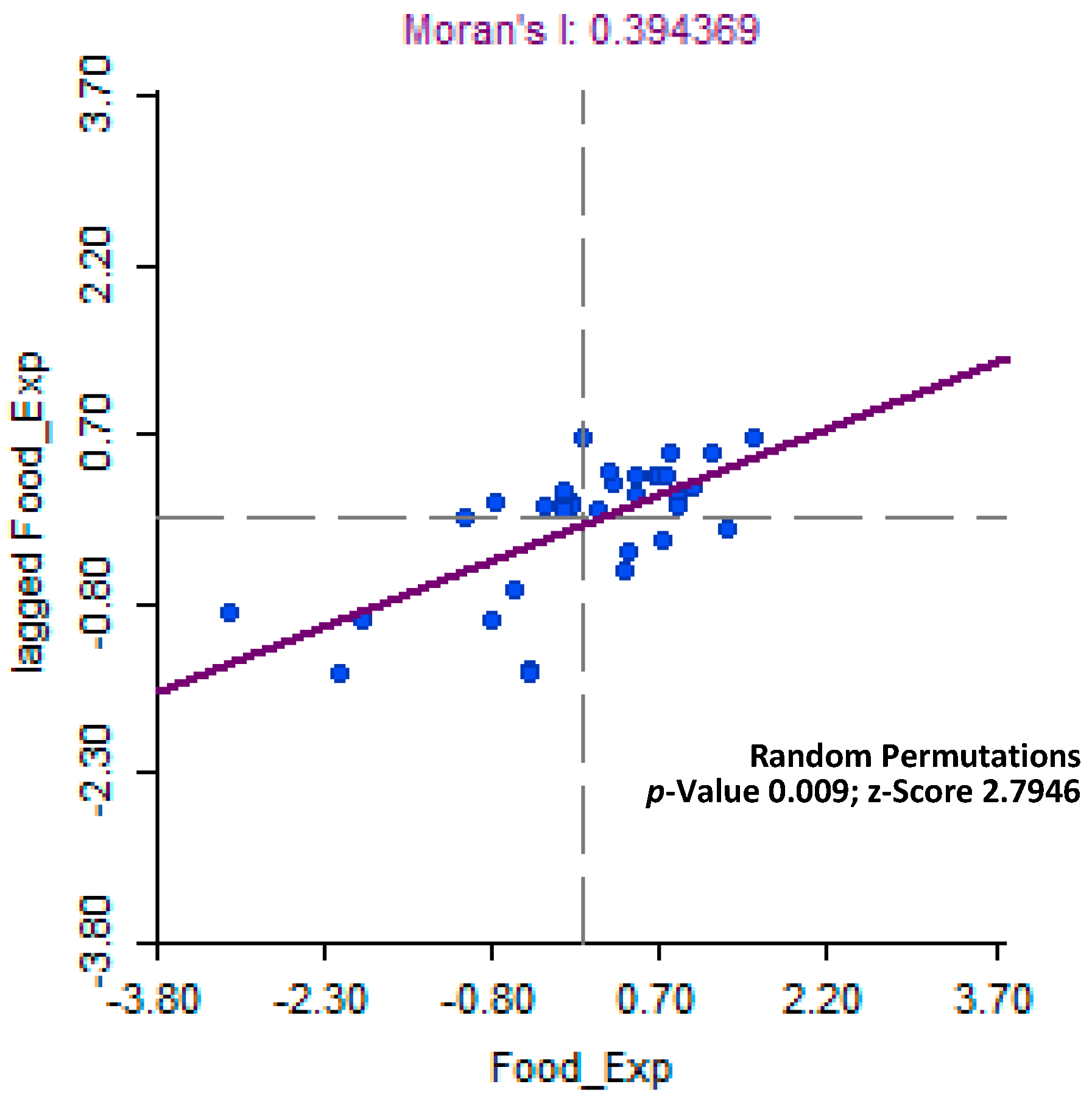
Spatial autocorrelation analysis was built on the background of the first geographic law, reflecting the degree of data interdependence from two spatial locations [51,52]. Spatial autocorrelation theory has been a key element in spatial research for over thirty years. Various spatial correlation measurements have been proposed so we can examine spatial analysis evolution from different perspectives [64,65,66,67,68,69]. Still, Moran’s I statistic has been commonly used as an indicator of global spatial autocorrelation [70]. It was firstly initiated by Moran [70] and Geary [71], which then popularized by Cliff and Ord [51]. The Moran scatter plot, first explained in Anselin [52,72], showing a plot with the y-axis of spatially lagged variable and the x-axis of the original variable. The slope of the line fit to the scatter plot equals to Moran’s I. In this study, we employed the Moran scatterplot by Anselin [72]. Moran’s index is defined by Equation (1) as follows:
I = i j W i j ( x i x ¯ ) ( x j x ¯ ) j ( x j x ¯ ) ,
where: I is the global Moran’s index, ranging between −1 and 1. Higher value of |I| indicate stronger spatial correlations, whereas a value close to zero indicate less autocorrelation. Additionally, n is the number of spatial units indexed by i and j; x refers to the variable; x ¯ denotes the mean of x; Wij is a matrix of spatial weights of unit i and j. As indicated by Glazier et al. [73], Moran I values > 0.2 or < −0.2 imply that there has been a significant spatial autocorrelation.
Global spatial autocorrelation merely describes the spatial characteristics of food expenditure throughout the nation. We extend this approach to the case of food expenditure variation by integrating a version of local indicators of spatial association (LISA) introduced by Anselin [74]. LISA was mainly used to analyze the correlation between a province and its neighbor [72,74] based on the Equation (2) as follows:
I i = n ( x i x ¯ ) i = 1 n ( x i x ¯ ) 2 i = 1 n w i j ( x i x ¯ ) ,
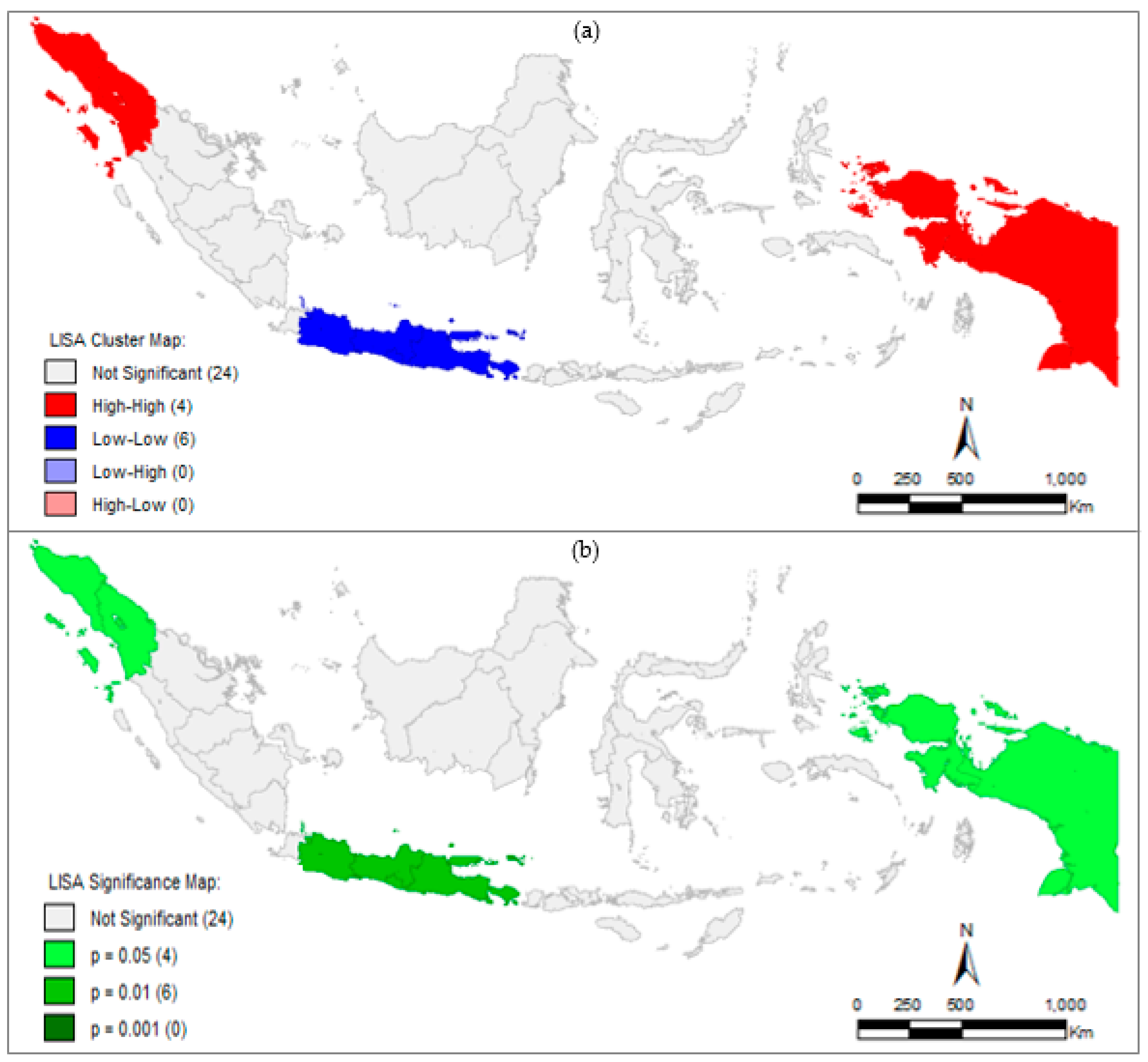
where: Ii represents the local Moran’s index of province i, n is the number of spatial units indexed by i and j; x refers to the variable; x ¯ denotes the mean of x, and Wij is a matrix of spatial weights of unit i and j. Regarding the value of this index, a cluster map of the province’s food expenditure can be clustered into (1) high–high clustering (H–H), showing provinces with high food expenditure surrounded by provinces with high food expenditure; (2) low–high clustering (L–H), showing provinces having low food expenditure surrounded by provinces with high food expenditure; (3) high–low clustering (H–L), showing provinces with high food expenditure surrounded by provinces with low food expenditure; (4) low–low clustering (L–L), showing provinces having low food expenditure surrounded by provinces having low food expenditure; and (5) not significant.

2.3.3. Spatial Econometrics Analysis

Spatial econometrics focuses on models that allow cross-sectional interactions between spatial units being studied. As panel data now become more available, the study of spatial econometrics becomes increasingly important. Since Cliff and Ord [51], economists have investigated cross-sectional models, especially spatial lag models. Anselin [52] and Griffith [75] discussed a wider range of methodological issues in spatial econometrics at more advanced levels. In this work, first, we estimated the standard regression specification by means of ordinary least square (OLS) based on Equation (3).
Y = β 0 + β 1 X 1 + β 2 X 2 + + ε ,
where: Y represents the food consumption expenditure, X represents the socio-economic indicators, β0 represents a constant term, β1 and β2 represent the regression coefficients, and ε represents the error term.
Second, we introduced the spatial lag model and the spatial error model. Compared to OLS, the spatial econometrics model considers spatial dependence in the regression model as OLS can’t be used to produce consistent estimates [76]. The spatial lag model (SLM) and the spatial error model (SEM) are part of spatial econometrics model which are commonly used. SLM assumes that there is a spatial dependence in the dependent variable, whereas SEM assumes that there is a spatial dependence in the error term. The reduced form of SLM can be seen in Equation (4):
Y = ρ W y + X β + ε ,
y = ( I n ρ W ) 1 X β + ( I n ρ W ) 1 ε ,
ε ~ N ( O n x 1 , σ 2 I n ) ,
where Y is an n × 1 vector of the dependent variable, n is observational units, W is a spatial contiguity matrix that describes the neighborhood pattern of spatial units in the sample, ρ is the spatial autoregression coefficient, X is an n × k matrix of explanatory variables, with an associated k x 1 regression coefficient vector β , and ε is a vector of random error. The n x 1 disturbance vector of ε is independent, normally distributed with a zero mean (0nx1) and having a constant variance ( σ 2 ). Furthermore, the specific form of SLM is shown in Equation (7).
Y i = α + ρ W i , j Y i + ε i ,
where: W i , j is an element of the spatial contiguity matrix. The W i , j Y i is a spatial variable that we constructed from the spatial contiguity matrix and the dependent variable, and the system is stationary. Thus, the model represents the spatial dependence structure of Y. This is a model that considers the effect of spatial autocorrelation in the dependent variable. Here, ρ is a parameter that relates the dependent variable of Y to the variable of the spatial weighted of Y.
On the other hand, SEM considers the spatial dependence in the error process and can be represented in Equation (8):
Y = X β + u ,
u = λ W u + ε ,
where: λ is the spatial autocorrelation coefficient.
The specific form of SEM is shown in Equation (10):
Y i = α i + β Y i + u i ,
μ i = λ j = 1 n w i j u i + ε i ,
Estimation of SLM and SEM coefficient was done by means of the maximum likelihood (ML), which was first outlined by Ord [52]. The starting point is the presumption of normality in terms of error. For models calculated using ML methods, statistics on the likelihood ratio test were used to resolve some model comparison for getting the best fit model. Testing alternative specifications for different spatial weight matrix or different sets of explanatory variables was also conducted [76].
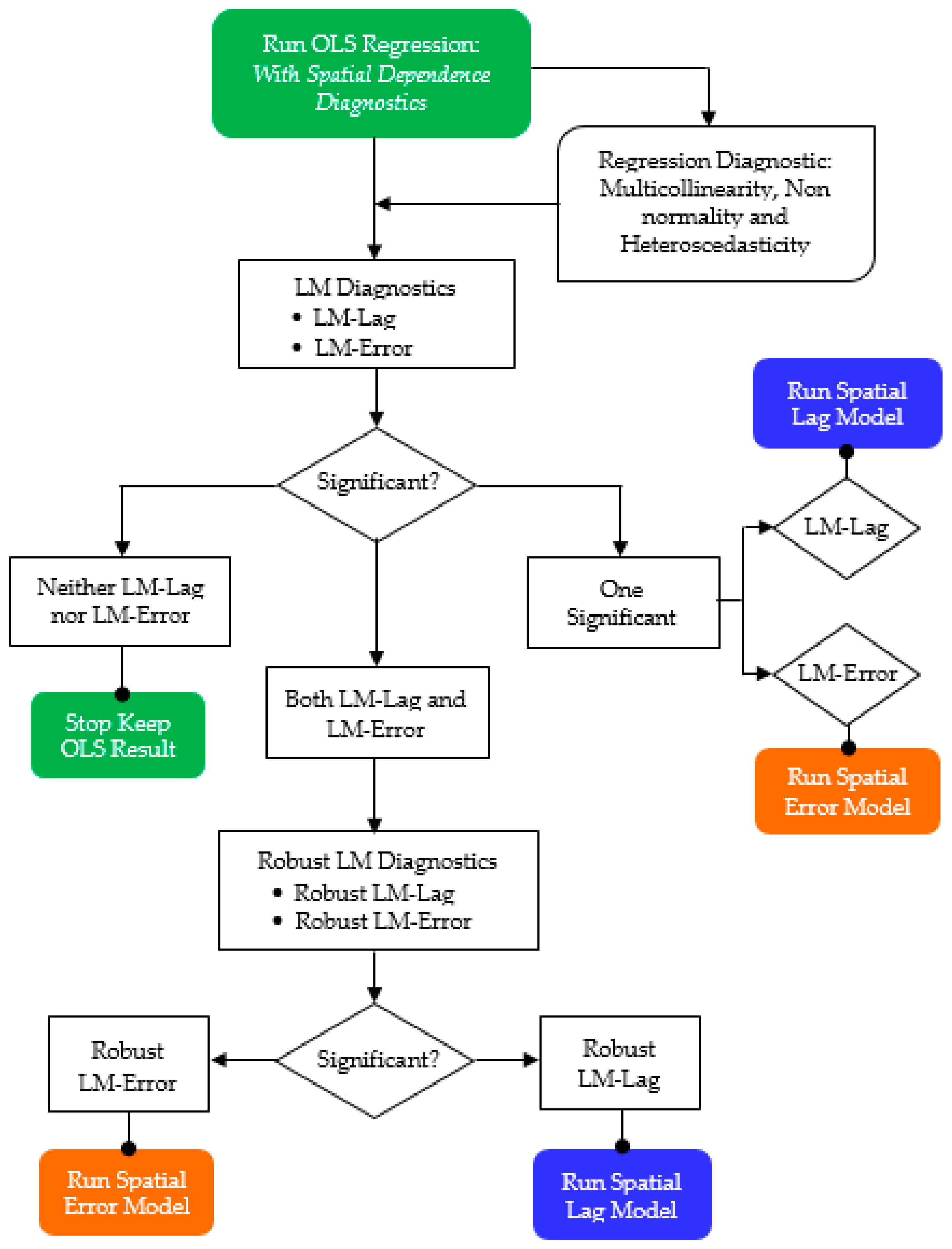
The array of spatial autocorrelation test statistics seems puzzling at first, but there is a way to proceed via the results towards a spatial regression specification. It is summarized in the diagnosis output of five Lagrange multiplier (LM) test statistics. The first two (LM-lag and robust LM-lag) are applied to test the fitness of the SLM. The next two (LM-error and robust LM-error) are applied to test the fitness of the SEM. The last test, LM-SARMA, is applied to measure the fitness of the model that considers both spatial lag and spatial error simultaneously. Then we decided which one is the most robust model based on those tests. We can see the whole process in the diagram shown in Figure 2.

2.4. Measures of Fit in Spatial Models

In order to measure the fitness of the spatial model, either SLM or SEM, there are four indicators that can be considered when the ML approach was used. They are consisting of: (1) the pseudo R2, (2) the maximized log-likelihood (LIK), (3) the Akaike information criterion (AIC) and (4) the Schwartz criterion (SC). The pseudo R2 is the ratio of the variance of the predicted values to the variance of the observed values for the dependent variable. It is different from R2 in the OLS model, which is calculated based on the decomposition of the total sum of squares into stated and residual sums of squares [77], but pseudo R2 still can be used to measure the fitness of the model. The higher the value of the pseudo R2 indicates that the model has better goodness of fit. While for LIK, AIC, and SC, the model has better goodness of fit when the value of LIK is higher, and the value of AIC and SC are lower.

3. Result

3.1. Spatial Variation of Food Consumption Expenditure and Socio-Economic Indicators by Provinces

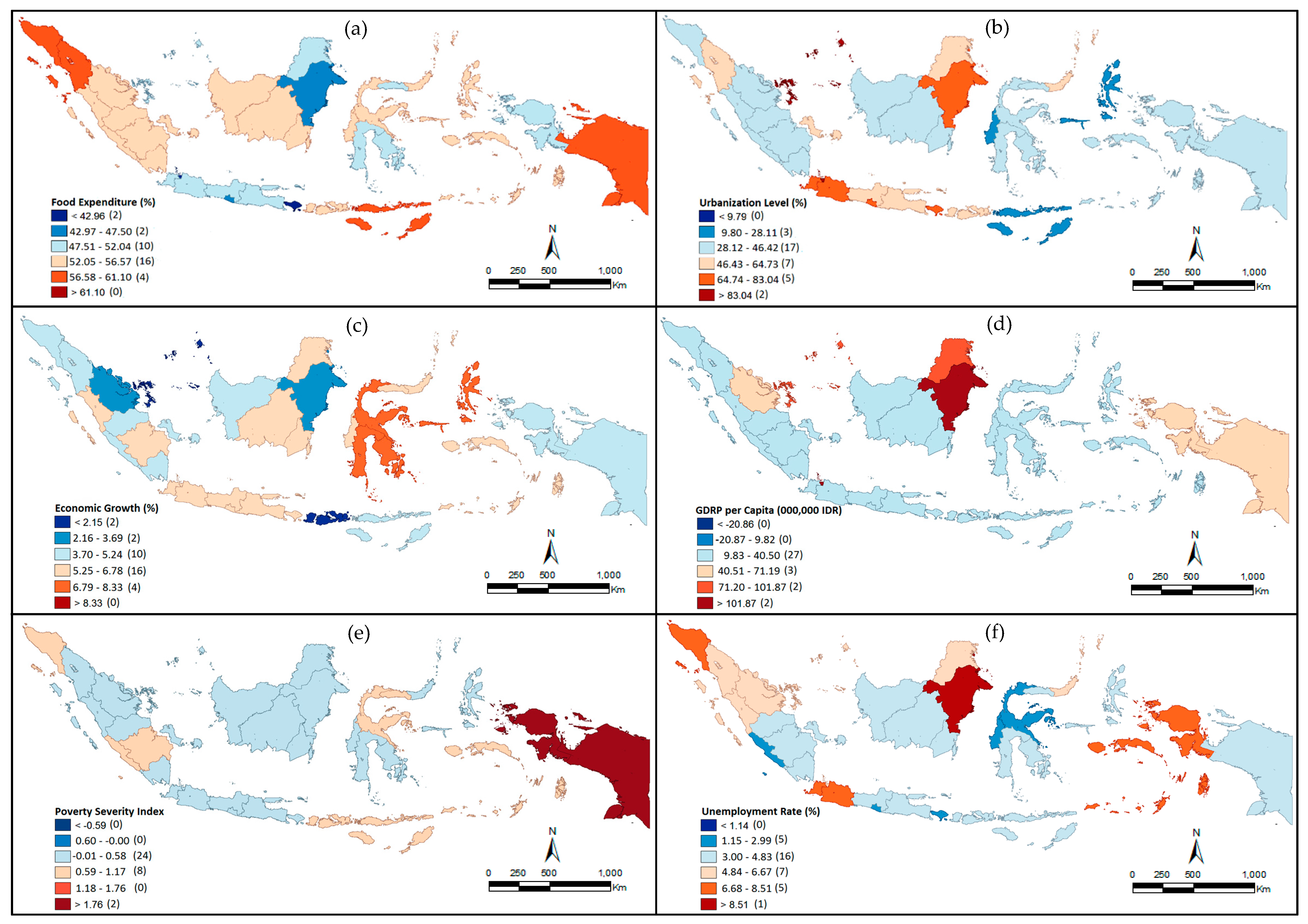
There are six variables of food expenditure and socio-economic indicators as mentioned in the method section. As noted, food expenditure here is a ratio of food expenditure per capita to total expenditure per capita showing the percentage value. Spatial variation of food expenditure (Figure 3a) shows that the highest value (56.58–61.10) found in the North part of Sumatra, Eastern Nusa Tenggara, and Eastern part of Papua. These regions are mostly dominated by rural areas, except the North Sumatra Province that showing a different pattern. The rest of Sumatra’s provinces, including some provinces in Kalimantan, Sulawesi, Maluku, and West Nusa Tenggara have values above average (orange colors) as they have so many areas which are still rural. Other regions including Java, Bali, East and North Kalimantan, South and Southeast Sulawesi, as well as West Papua have food expenditure below the average (blue colors). Most prominent and populous cities are located in these regions. These phenomena show that rural areas have higher percentage of food expenditure, whereas urban areas have lower percentage of food expenditure.
Then Figure 3b shows that the highest urbanization (64.74–83.04) occurred in Western Java, Yogyakarta, Bali, and the East Kalimantan Province. These regions actually are populous areas that having many cities. Other regions that have an urbanization rate above average (orange colors) consist of North Sumatra Province, the rest of Java, West Nusa Tenggara Province, and North Kalimantan Province as well as North Sulawesi Province. These regions also have many urbanized areas. Rest of regions have urbanization below average (blue colors) and these regions were actually dominated by rural areas.
Figure 3c shows that economic growth above average (orange colors) mostly found in Java, South and West Sumatra Province, Central, South and North Kalimantan Province, the whole Sulawesi, and Maluku. Some of these regions are urbanized areas with high economic activities such as Java, other regions are rich with natural resources such as marine biota, plantation, and mining, except Bali which is known as a global tourism destination. Other regions have economic growth below average (blue colors). Some of them have a lack of development and natural resources such as West and East Nusa Tenggara. Surprisingly, regions that are known having rich natural resources including coal, gas, and oil such as East Kalimantan, Riau Provinces, and Papua have low economic growth. Seemingly the economic growth of these regions that have been relying too much on natural resources has become stagnant now.
The variation of GDRP per capita between provinces is shown in Figure 3d. There are only seven provinces that have GDRP per capita above average (orange colors) consisting of Riau, Riau Islands, Jakarta, East Kalimantan, North Kalimantan, West Papua, and Papua Province. Except for Jakarta, these regions are rich with natural resources, mainly mining, but having less population. As shown in Figure 3c, most of these regions have low economic growth, thus people are not interested to come and involve in economic activities in these regions. Seemingly, the regional leakage phenomenon has occurred in these regions.
Figure 3e shows the distribution of poverty between provinces. The highest poverty (> 1.76) found in Papua beyond other provinces. This phenomenon shows that the development of people’s prosperity in Papua is still lacking than other provinces in Indonesia. Other provinces have poverty slightly above average (light orange color) and slightly below average (light blue colors); thus, the difference is not significant.
The distribution of unemployment is shown in Figure 3f. The distribution is quite random. Higher unemployment (orange colors) found in Western Java, Northern Sumatra, Eastern Kalimantan, Northern Sulawesi, Southern Maluku, and Western Papua. This shows that unemployment above-average found in more developed areas such as Western Java, in the area with rich natural resources such as some parts of Kalimantan and Sumatra also Northern part of Sulawesi, and the area with lack of economic development such as Southern Maluku and Western Papua.

3.2. Global and Local Spatial Autocorrelation

Moran’s index of food expenditure is greater than 0 (Figure 4), indicating that food expenditure presents positive spatial autocorrelations. Additionally, as the p-value is less than 0.05 with a positive z-score [51,78], it can be concluded that the value of this variable is spatial. As shown by the LISA map of food expenditure, 10 provinces have statistically significant spatial clustering, and 24 provinces have insignificant spatial autocorrelation (Figure 5). Specifically, the number of provinces showing H–H and L–L cluster are 4 and 6, respectively, and there are no provinces showing L–H and H–L. In terms of geographical distribution, H–H is found in four provinces consisting of Aceh and North Sumatera in Sumatra Island and Papua and West Papua Province in Papua Island, while L–L is located only in one Island (Java-Bali) at six provinces (DKI Jakarta, West Java, Central Java, DI Yogyakarta, East Java, and Bali). This result indicated that spatial autocorrelation is exist between food expenditures of provinces, therefore, a spatial regression approach is required.

3.3. Evidence from Spatial Econometrics Modeling

The above analysis of global and local spatial autocorrelation shows that spatial clustering exists at the province-level of food expenditure. Therefore, further analysis is required in the form of a spatial econometrics model that takes spatial dependence into consideration. Table 1 shows the results of the OLS estimation of the food expenditure model, as the preliminary step to develop spatial econometrics model. This model has R2 value of 0.6688. In addition, the other three measurements of the goodness of fit are included, thus we can compare the fitness of this model with the spatial regression models. They consist of the log-likelihood (−80.354), the Akaike information criterion (172.708), and the Schwarz criterion (181.866).
The OLS coefficient shows that economic growth, GDRP per capita, poverty severity index, and urbanization have negative coefficients, meaning that increasing their value are able to decline food expenditure. Economic growth shows the highest value of coefficient than others, thus it has the highest effect on food expenditure. Furthermore, from those four variables, only the poverty severity index does not have a significant effect (p-value > 0.05). On the other hand, the unemployment rate has a positive coefficient showing that increasing unemployment will increase food expenditure. Therefore, the success of development planning in improving economic growth, GDRP per capita, as well as urbanization are able to decline food expenditure as long as this is accompanied by efforts to reduce unemployment.
A test for non-normality (Jarque–Bera) score (0.008; p = 0.996) indicates the normal distribution of an error term and the low p-value of Breusch–Pagan test points (18.819; p = 0.002) shows the existence of heteroskedasticity. In addition, the matrix correlation coefficient among independent variables was calculated in order to eliminate multicollinearity. According to Anselin and Rey [77], the multicollinearity condition number below 30 showing an absence of multicollinearity (Table 2).
Afterward, Table 3 shows that the LM-LAG of the food expenditure model is more significant than LM-error (see the p-value that should be less than 0.05 for the significance). According to Anselin [77], this indicates that food expenditure is not distributed randomly, but is spatially correlated. Therefore, we should develop the spatial lag model (SLM) in modeling food expenditure.
Table 4 shows the results of the SLM in modeling food expenditure. For the lag model, a new variable for the spatial lag coefficient called “W_Food Expenditure” was introduced to the model. Its coefficient parameter (ρ) reflects the effect of spatial dependence within our sample data, measuring the average influence of neighboring observations on a certain observation. It has a negative effect and it is highly significant, indicating that there is a contrary effect between neighbors. For other variables actually still show similar signs of coefficients as the OLS, but now the effect of increasing poverty severity index on declining food expenditure becomes significant and higher than economic growth, GDRP per capita, and urbanization. Therefore, the poverty issue should be of concern. While the unemployment rate still has a positive coefficient as the OLS model, the absolute value of its coefficient is now approaching the absolute value of the coefficient of economic growth. Again, the effect of the unemployment rate on food expenditure should not be neglected.
Regarding the fitness of the model, the value listed in the spatial lag output is not a real R2, but so-called a pseudo-R2. Still, it can be seen that the SLM model has an increase in R2 thus this model is likely better than OLS. The proper measures of fit are the Log-likelihood, AIC (Akaike info criterion), and SC. We notice an increase in the Log-likelihood from -80.354 (for OLS) to -75.306. Furthermore, the AIC and SC are decreasing from 172.708 (OLS) to 164.611, and from 181.866 (OLS) to 175.296, respectively. All of these values are suggesting an improvement in the model fitness after the spatial lag approach was used.

4. Discussion and Conclusions

In general, the spatial distribution of food expenditure between provinces shows a closer pattern with the spatial distribution of urbanization and economic growth. Although not all urbanized areas exhibit lower food expenditure, there is a pattern where higher urbanization is likely followed by lower food expenditure. Similarly, higher economic growth found in most urban areas, but still, there are some rural areas with rich natural resources that are able to decline food expenditure. In this case, the Engels’ law seems to work properly as more prosperous society spend a lesser income proportion for food consumption.
The distribution of other variables has more random patterns. Regarding GDRP per capita except for DKI Jakarta, all provinces with a higher value of GDRP per capita found in provinces that have rich natural resources but have less population. According to the poverty severity index, Papua has the highest value beyond other provinces that more or less have similar value. Whereas a higher unemployment rate can be found in more scattered areas, including provinces which have high urbanization level or rich natural resources or retarded development.
Since the patterns are not clear enough, then further approach is required, particularly a regression. As the connectivity between provinces should be considered, the first step that was done is to check the presence of spatial dependence in the food expenditure variable. The results show that spatial correlation in food expenditure between provinces significantly exists based on the calculation of the Moran Index for global and LISA for local spatial autocorrelation. Interestingly for LISA results, high–high cluster found in rural or regions with a lack of development such as the northern part of Sumatra and Papua, where both regions are actually rich with natural resources. In addition, the low–low cluster is only found in Java as an urbanized island [79] where all economic activities are concentrated. Again, urbanization and economic growth show important roles in lessening the proportion of income for food expenditure.
Then, the OLS regression was developed as a step toward building the SLM model. The absolute values of the SLM coefficient show that the poverty severity index has the highest effect followed by economic growth, unemployment rate, w food expenditure, urbanization, and GDRP per capita, respectively. Except unemployment rate variable, all variables have negative coefficients, which mean their increase will decline the share of food expenditure. Surely, increasing economic growth, urbanization, and GDRP per capita are expected as they are able to reduce food expenditure as consequences of increasing income and prosperity. However, for the poverty severity index, the situation is different. Against Engel’s law, a lower share of food expenditure also occurs when income disparity among the poor is increasing. Since this variable has the highest coefficient value; thus, the poverty issue will reduce the benefit of other variables such as economic growth, urbanization, and GDRP per capita. Food expenditure variable also has a negative coefficient indicating that there is a contrary effect between province and its neighbor where lowering food expenditure in a province followed by increasing food expenditure in its neighbor, and vice versa. This implies that imbalanced development between provinces will push inequality in food expenditure between provinces. Therefore, the balanced development becomes very important, meaning that disparity in economic growth, GDRP per capita, urbanization, including poverty and unemployment issues between provinces should be reduced.
Particularly for the unemployment rate, it should be of concern that increasing the unemployment rate is followed by increasing food expenditure. Seemingly, unemployed have a lack of income or budget, so that they must spend most of their money on buying food. Although the coefficient value of the unemployment rate is below economic growth, it still can considerably reduce the benefit of increasing economic growth, urbanization, and GDRP per capita.
Based on these findings, poverty and unemployment rate are critical issues that should be addressed to optimize the capability of economic growth, urbanization, and GDRP per capita in reducing food expenditure as well as enhancing food security. Previous research shows that urbanization has pushed economic development [80], and has positive impacts on economic growth [81,82]. On the other hand, increasing income disparity among the poor result in declining food expenditure, seemingly caused by an urgent need for fulfilling basic non-food expenditure, thus reducing income for buying food [83]. Furthermore, increasing food expenditure due to rising unemployment has likely occurred, as explained by Carroll et al. [37] that at the time of unemployment, food expenditure is highly dependent on the savings owned. Lack of savings will make unemployed should prioritize food than other things; thus, most of their income is spent on food expenditure.
In conclusion, increasing economic growth, urbanization, and GDRP per capita are able to support food security by increasing income. Thus, the household consumption is shifted from food consumption to non-food consumption, causing lower food expenditure. This phenomenon certainly supports the Engel’s law. Contrarily, the Engel’s law will be violated due to three other variables consisting of poverty, unemployment, and regional development disparity. The severity of poverty will lead to a misleading conclusion as lower food expenditures is also occurred when people’s ability to purchase is very low. Unemployed people will not get any benefit from economic growth, thus they become vulnerable to food insecurity as they spend most of their income on food. Furthermore, regional development disparity will make a decline in food expenditure only occurred in provinces with higher economic growth, urbanization, and GDRP per capita (economic growth centers).
Those above findings highlight more comprehensive factors that affect the application of Engel’s law. Depending on the situation in every country or region, the benefit of regional economic development on supporting food availability and accessibility will depend on their capability to manage poverty, unemployment, and regional disparity issues. This gives a new understanding of Engel’s law that might be applied differently depending on different socio-economic factors that determine the share of food expenditure, instead of debating the evidence that support or not support the Engel’s law.
Understanding about food expenditure is very important to a wide range of economy and policy research, including consumption and demand behavior research, as well as living standards, poverty, and inequality [84,85,86,87]. Furthermore, food security issue has become crucial as recently it has been included as one of SDG’s target to end hunger and improve food nutrition that should be consumed. Still, this study has a limitation that should be considered in conducting future studies. The analysis of the study was based on the provincial-level data. We encourage future researchers to broaden the scope of this research by using data at the city or district level. An interesting idea for further research is by conducting a similar spatial analysis on more wide socio-economic factors that affect food consumption, such as non-food expenditure, dietary habits, and population composition based on gender and age.

Author Contributions

A.S.P. designed the research, collected, and analyzed the data. A.S.P. and D.O.P. Software. G.T. supervision. All authors wrote, reviewed and commented on the manuscript. All authors have read and approved the final manuscript. All authors contributed equally to this work.

Funding

The research was supported by "One Belt and One Road" initiative on the implementation mechanism of agricultural capacity cooperation between China and countries along the route (18JLD310), the Heilongjiang Provincial Philosophy and Social Science Office, and a Ph.D. scholarship from the China Scholarship Council (CSC), the China Government, for the first author.

Acknowledgments

Thank you to editor and all reviewers for their valuable advice on this paper.

Conflicts of Interest

The authors declare no conflicts of interest. The funders had no role in the design of the study; in the collection, analyses, or interpretation of data; in the writing of the manuscript, or in the decision to publish the results.

References

  1. FAO. Rome Declaration on World Food Security and World Food Summit Plan of Action: World Food Summit 13–17 November 1996, Rome, Italy; FAO: Rome, Italy, 1996; ISBN 9251039399. [Google Scholar]
  2. Abu Hatab, A.; Cavinato, M.E.R.; Lagerkvist, C.J. Urbanization, livestock systems and food security in developing countries: A systematic review of the literature. Food Secur. 2019, 11, 279–299. [Google Scholar] [CrossRef] [Green Version]
  3. Abu Hatab, A.; Cavinato, M.E.R.; Lindemer, A.; Lagerkvist, C.J. Urban sprawl, food security and agricultural systems in developing countries: A systematic review of the literature. Cities 2019, 94, 129–142. [Google Scholar] [CrossRef]
  4. Haysom, G.; Tawodzera, G. Measurement drives diagnosis and response: Gaps in transferring food security assessment to the urban scale. Food Policy 2018, 74, 117–125. [Google Scholar] [CrossRef]
  5. Regmi, A.; Meade, B. Demand side drivers of global food security. Glob. Food Secur. 2013, 2, 166–171. [Google Scholar] [CrossRef] [Green Version]
  6. Satterthwaite, D.; McGranahan, G.; Tacoli, C. Urbanization and its implications for food and farming. Philos. Trans. R. Soc. B Biol. Sci. 2010, 365, 2809–2820. [Google Scholar] [CrossRef]
  7. He, C.; Liu, Z.; Xu, M.; Ma, Q.; Dou, Y. Urban expansion brought stress to food security in China: Evidence from decreased cropland net primary productivity. Sci. Total Environ. 2017, 576, 660–670. [Google Scholar] [CrossRef]
  8. Li, H.; Wu, Y.; Huang, X.; Sloan, M.; Skitmore, M. Spatial-temporal evolution and classification of marginalization of cultivated land in the process of urbanization. Habitat Int. 2017, 61, 1–8. [Google Scholar] [CrossRef] [Green Version]
  9. Wang, J.; Lin, Y.; Glendinning, A.; Xu, Y. Land-use changes and land policies evolution in China’s urbanization processes. Land Use Policy 2018, 75, 375–387. [Google Scholar] [CrossRef]
  10. Van Vliet, J.; Eitelberg, D.A.; Verburg, P.H. A global analysis of land take in cropland areas and production displacement from urbanization. Glob. Environ. Chang. 2017, 43, 107–115. [Google Scholar] [CrossRef]
  11. Sklenicka, P.; Janovska, V.; Salek, M.; Vlasak, J.; Molnarova, K. The Farmland Rental Paradox: Extreme land ownership fragmentation as a new form of land degradation. Land Use Policy 2014, 38, 587–593. [Google Scholar] [CrossRef]
  12. Sklenicka, P. Classification of farmland ownership fragmentation as a cause of land degradation: A review on typology, consequences, and remedies. Land Use Policy 2016, 57, 694–701. [Google Scholar] [CrossRef] [Green Version]
  13. Liu, Y.; Yamauchi, F. Population density, migration, and the returns to human capital and land: Insights from Indonesia. Food Policy 2014, 48, 182–193. [Google Scholar] [CrossRef] [Green Version]
  14. Masters, W.A.; Djurfeldt, A.A.; De Haan, C.; Hazell, P.; Jayne, T.; Jirström, M.; Reardon, T. Urbanization and farm size in Asia and Africa: Implications for food security and agricultural research. Glob. Food Secur. 2013, 2, 156–165. [Google Scholar] [CrossRef]
  15. Rudiarto, I.; Hidayani, R.; Fisher, M. The bilocal migrant: Economic drivers of mobility across the rural-urban interface in Central Java, Indonesia. J. Rural Stud. 2019. [Google Scholar] [CrossRef]
  16. Yin, X.; Chen, J.; Li, J. Rural innovation system: Revitalize the countryside for a sustainable development. J. Rural Stud. 2019. [Google Scholar] [CrossRef]
  17. Parry, M.L.; Rosenzweig, C.; Iglesias, A.; Livermore, M.; Fischer, G. Effects of climate change on global food production under SRES emissions and socio-economic scenarios. Glob. Environ. Chang. 2004, 14, 53–67. [Google Scholar] [CrossRef]
  18. White, J.W.; Hoogenboom, G.; Kimball, B.A.; Wall, G.W. Methodologies for simulating impacts of climate change on crop production. Field Crop Res. 2011, 124, 357–368. [Google Scholar] [CrossRef] [Green Version]
  19. Hijmans, R.J. The effect of climate change on global potato production. Am. J. Potato Res. 2003, 80, 271–279. [Google Scholar] [CrossRef]
  20. Ludwig, F.; Asseng, S. Climate change impacts on wheat production in a Mediterranean environment in Western Australia. Agric. Syst. 2006, 90, 159–179. [Google Scholar] [CrossRef]
  21. FAO. Food security. Policy Brief. 2006, 2, 1–4. [Google Scholar]
  22. Lusk, J.L. Income and (Ir) rational food choice. J. Econ. Behav. Organ. 2019, 166, 630–645. [Google Scholar] [CrossRef]
  23. Diehl, J.A.; Oviatt, K.; Chandra, A.J.; Kaur, H. Household food consumption patterns and food security among low-income migrant urban farmers in Delhi, Jakarta, and Quito. Sustainability 2019, 11, 1378. [Google Scholar] [CrossRef] [Green Version]
  24. Gerbens-Leenes, P.W.; Nonhebel, S.; Krol, M.S. Food consumption patterns and economic growth. Increasing affluence and the use of natural resources. Appetite 2010, 55, 597–608. [Google Scholar] [CrossRef] [PubMed]
  25. Marques, A.C.; Fuinhas, J.A.; Pais, D.F. Economic growth, sustainable development and food consumption: Evidence across different income groups of countries. J. Clean. Prod. 2018, 196, 245–258. [Google Scholar] [CrossRef]
  26. Gandhi, V.P.; Zhou, Z. Food demand and the food security challenge with rapid economic growth in the emerging economies of India and China. Food Res. Int. 2014, 63, 108–124. [Google Scholar] [CrossRef]
  27. Burggraf, C.; Kuhn, L.; Zhao, Q.; Teuber, R.; Glauben, T. Economic growth and nutrition transition: An empirical analysis comparing demand elasticities for foods in China and Russia. J. Integr. Agric. 2015, 14, 1008–1022. [Google Scholar] [CrossRef]
  28. Pingali, P. Westernization of Asian diets and the transformation of food systems: Implications for research and policy. Food Policy 2007, 32, 281–298. [Google Scholar] [CrossRef]
  29. Huang, J.; Bouis, H. Structural Changes in the Demand for Food in Asia; Int. Food Policy Res. Inst.: Washington, DC, USA, 1996. [Google Scholar]
  30. Kearney, J. Food consumption trends and drivers. Philos. Trans. R. Soc. B Biol. Sci. 2010, 365, 2793–2807. [Google Scholar] [CrossRef]
  31. Stage, J.; Stage, J.; Mcgranahan, G. Is urbanization contributing to higher food prices? Environ. Urban. 2010, 22, 199–215. [Google Scholar] [CrossRef]
  32. Szabo, S. Urbanisation and Food Insecurity Risks: Assessing the Role of Human Development. Oxf. Dev. Stud. 2016, 44, 28–48. [Google Scholar] [CrossRef] [Green Version]
  33. Dávila, O.G. Food security and poverty in Mexico: The impact of higher global food prices. Food Secur. 2010, 2, 383–393. [Google Scholar] [CrossRef]
  34. Kam, S.P.; Hossain, M.; Bose, M.L.; Villano, L.S. Spatial patterns of rural poverty and their relationship with welfare-influencing factors in Bangladesh. Food Policy 2005, 30, 551–567. [Google Scholar] [CrossRef]
  35. Maitra, C.; Rao, D.S.P. Poverty-Food Security Nexus: Evidence from a Survey of Urban Slum Dwellers in Kolkata. World Dev. 2015, 72, 308–325. [Google Scholar] [CrossRef]
  36. Gibney, M.J.; Lee, P. Patterns of food and nutrient intake in a suburb of Dublin with chronically high unemployment. J. Hum. Nutr. Diet. 1993, 6, 13–22. [Google Scholar] [CrossRef]
  37. Carroll, C.D.; Dynan, K.E.; Krane, S.D. Unemployment risk and precautionary wealth: Evidence from households’ balance sheets. Rev. Econ. Stat. 2003, 85, 586–604. [Google Scholar] [CrossRef] [Green Version]
  38. Aguiar, M.; Hurst, E. Consumption versus expenditure. J. Political Econ. 2005, 113, 919–948. [Google Scholar] [CrossRef] [Green Version]
  39. Etana, D.; Tolossa, D. Unemployment and Food Insecurity in Urban Ethiopia. Afr. Dev. Rev. 2017, 29, 56–68. [Google Scholar] [CrossRef]
  40. Antelo, M.; Magdalena, P.; Reboredo, J.C. Economic crisis and the unemployment effect on household food expenditure: The case of Spain. Food Policy 2017, 69, 11–24. [Google Scholar] [CrossRef] [Green Version]
  41. Leonard, T.; McKillop, C.; Carson, J.A.; Shuval, K. Neighborhood effects on food consumption. J. Behav. Exp. Econ. 2014, 51, 99–113. [Google Scholar] [CrossRef] [Green Version]
  42. Farrow, A.; Larrea, C.; Hyman, G.; Lema, G. Exploring the spatial variation of food poverty in Ecuador. Food Policy 2005, 30, 510–531. [Google Scholar] [CrossRef] [Green Version]
  43. Morrison, K.T.; Nelson, T.A.; Ostry, A.S. Mapping spatial variation in food consumption. Appl. Geogr. 2011, 31, 1262–1267. [Google Scholar] [CrossRef]
  44. Cerciello, M.; Garofalo, A. Estimating urban food waste at the local level: Are good practices in food consumption persistent? Econ. Politica 2018, 36, 863–886. [Google Scholar] [CrossRef]
  45. Case, A.C. Spatial patterns in household demand. Econom. J. Econom. Soc. 1991, 59, 953–965. [Google Scholar] [CrossRef] [Green Version]
  46. Aten, B.H. Does space matter? International comparisons of the prices of tradables and nontradables. Int. Reg. Sci. Rev. 1997, 20, 35–52. [Google Scholar] [CrossRef]
  47. Murdoch, J.C.; Rahmatian, M.; Thayer, M.A. A spatially autoregressive median voter model of recreation expenditures. Public Financ. Q. 1993, 21, 334–350. [Google Scholar] [CrossRef]
  48. Bell, K.P.; Bockstael, N.E. Applying the generalized-moments estimation approach to spatial problems involving micro-level data. Rev. Econ. Stat. 2000, 82, 72–82. [Google Scholar] [CrossRef]
  49. Pinkse, J.; Slade, M.E. Contracting in space: An application of spatial statistics to discrete-choice models. J. Econom. 1998, 85, 125–154. [Google Scholar] [CrossRef]
  50. Kelejian, H.H.; Prucha, I.R. A generalized moments estimator for the autoregressive parameter in a spatial model. Int. Econ. Rev. 1999, 40, 509–533. [Google Scholar] [CrossRef] [Green Version]
  51. Cliff, A.D.; Ord, J.K. Spatial Autocorrelation; Pion: London, UK, 1973. [Google Scholar]
  52. Anselin, L. Spatial Econometrics: Methods and Models; Kluwer Academic Publishers: Boston, MA, USA, 1988. [Google Scholar]
  53. Tobler, W. On the First Law of Geography: A Reply. Ann. Assoc. Am. Geogr. 2004, 94, 304–310. [Google Scholar] [CrossRef]
  54. Bappenas. Rencana Pembangunan Jangka Menengah Nasional (RPJMN) 2015–2019; Bappenas: Jakarta, Indonesia, 2015. [Google Scholar]
  55. Pribadi, D.O.; Putra, A.S.; Rustiadi, E. Determining optimal location of new growth centers based on LGP–IRIO model to reduce regional disparity in Indonesia. Ann. Reg. Sci. 2015, 54, 89–115. [Google Scholar] [CrossRef]
  56. Houthakker, H.S. An international comparison of household expenditure patterns, commemorating the centenary of Engel’s law. Econom. J. Econom. Soc. 1957, 59, 532–551. [Google Scholar] [CrossRef]
  57. Seale, J.L., Jr.; Regmi, A. Modeling international consumption patterns. Rev. Income Wealth 2006, 52, 603–624. [Google Scholar] [CrossRef]
  58. John Baffes, B.; Etienne, X.L. Analysing food price trends in the context of Engel’s Law and the Prebisch-Singer hypothesis. Oxf. Econ. Pap. 2016, 68, 688–713. [Google Scholar] [CrossRef]
  59. Hamilton, B.W. Using Engel’s Law to estimate CPI bias. Am. Econ. Rev. 2001, 91, 619–630. [Google Scholar] [CrossRef]
  60. Kaus, W. Beyond Engel’s law-A cross-country analysis. J. Socio-Econ. 2013, 47, 118–134. [Google Scholar] [CrossRef]
  61. Grigg, D. Food Expenditure and Economic Development. GeoJournal 1994, 33, 377–382. [Google Scholar]
  62. Brunsdon, C.; Fotheringham, A.S.; Charlton, M.E. Geographically weighted regression: A method for exploring spatial nonstationarity. Geogr. Anal. 1996, 28, 281–298. [Google Scholar] [CrossRef]
  63. GeoDa Center. Available online: https://geodacenter.github.io/ (accessed on 3 June 2019).
  64. Getis, A. Spatial weights matrices. Geogr. Anal. 2009, 41, 404–410. [Google Scholar] [CrossRef]
  65. Haining, R.P. Spatial autocorrelation and the quantitative revolution. Geogr. Anal. 2009, 41, 364–374. [Google Scholar] [CrossRef]
  66. Xu, C.; Pribadi, D.O.; Haase, D.; Pauleit, S. Incorporating spatial autocorrelation and settlement type segregation to improve the performance of an urban growth model. Environ. Plan. B Urban Anal. City Sci. 2018. [Google Scholar] [CrossRef]
  67. Zhao, X.; Zheng, Y.; Huang, X.; Kwan, M.P.; Zhao, Y. The effect of urbanization and farmland transfer on the spatial patterns of non-grain farmland in China. Sustainability 2017, 9, 1438. [Google Scholar] [CrossRef] [Green Version]
  68. Zhao, R.; Tian, Y.; Lei, A.; Boadu, F.; Ren, Z. The effect of local government debt on regional economic growth in China: A nonlinear relationship approach. Sustainability 2019, 11, 3065. [Google Scholar] [CrossRef] [Green Version]
  69. Wang, K.; Zhang, J.; Geng, Y.; Xiao, L.; Xu, Z. Differential Spatial-Temporal Responses of Carbon Dioxide Emissions to Economic Development: Empirical Evidence Based on Spatial Analysis. Mitig. Adapt. Strateg. Glob. Chang. 2019, 24, 1–24. [Google Scholar] [CrossRef]
  70. Moran, P.A.P. The interpretation of statistical maps. J. R. Stat. Soc. Ser. B (Methodol.) 1948, 10, 243–251. [Google Scholar] [CrossRef]
  71. Geary, R.C. The contiguity ratio and statistical mapping. Inc. Stat. 1954, 5, 115–146. [Google Scholar] [CrossRef]
  72. Anselin, L. The Moran Scatterplot as an ESDA Tool to Assess Local Instability in Spatial Association; Regional Research Institute, West Virginia University Morgantown: Morgantown, WV, USA, 1993. [Google Scholar]
  73. Glazier, R.H.; Creatore, M.I.; Gozdyra, P.; Matheson, F.I.; Steele, L.S.; Boyle, E.; Moineddin, R. Geographic methods for understanding and responding to disparities in mammography use in Toronto, Canada. J. Gen. Intern. Med. 2004, 19, 952–961. [Google Scholar] [CrossRef] [PubMed] [Green Version]
  74. Anselin, L. Local indicators of spatial association—LISA. Geogr. Anal. 1995, 27, 93–115. [Google Scholar] [CrossRef]
  75. Griffith, D.A. Advanced spatial statistics for analysing and visualizing geo-referenced data. Int. J. Geogr. Inf. Sci. 1993, 7, 107–123. [Google Scholar] [CrossRef]
  76. LeSage, J.; Pace, R.K. Introduction to Spatial Econometrics; CRC Press Taylor & Francis Group: Boca Raton, FL, USA, 2009. [Google Scholar]
  77. Anselin, L.; Rey, J.S. Modern Spatial Econometrics in Practice; GeoDa Press LLC: Chicago, IL, USA, 2014. [Google Scholar]
  78. Cliff, A.D.; Ord, J.K. Spatial Processes: Models & Applications; Pion: London, UK, 1981. [Google Scholar]
  79. BPS (Indonesia Statistical Office). Statistical Yearbook of Indonesia 2018; BPS: Jakarta, Indonesia, 2018. [Google Scholar]
  80. Gallup, J.L.; Sachs, J.D.; Mellinger, A.D. Geography and economic development. Int. Reg. Sci. Rev. 1999, 22, 179–232. [Google Scholar] [CrossRef]
  81. Frenken, K.; Van Oort, F.; Verburg, T. Related variety, unrelated variety and regional economic growth. Reg. Stud. 2007, 41, 685–697. [Google Scholar] [CrossRef] [Green Version]
  82. Turok, I.; McGranahan, G. Urbanization and economic growth: The arguments and evidence for Africa and Asia. Environ. Urban. 2013, 25, 465–482. [Google Scholar] [CrossRef]
  83. Haughton, J.; Khandker, S.R. Handbook on Poverty+ Inequality; World Bank Publications: Washington, DC, USA, 2009; ISBN 0821376144. [Google Scholar]
  84. Zezza, A.; Carletto, C.; Fiedler, J.L.; Gennari, P.; Jolliffe, D. Food counts. Measuring food consumption and expenditures in household consumption and expenditure surveys (HCES). Introduction to the special issue. Food Policy 2017, 72, 1–6. [Google Scholar] [CrossRef]
  85. Borlizzi, A.; Delgrossi, M.E.; Cafiero, C. National food security assessment through the analysis of food consumption data from Household Consumption and Expenditure Surveys: The case of Brazil’s Pesquisa de Orçamento Familiares 2008/09. Food Policy 2017, 72, 20–26. [Google Scholar] [CrossRef]
  86. Brzozowski, M.; Crossley, T.F.; Winter, J.K. A comparison of recall and diary food expenditure data. Food Policy 2017, 72, 53–61. [Google Scholar] [CrossRef] [Green Version]
  87. Ansah, I.G.K.; Gardebroek, C.; Ihle, R. Resilience and household food security: A review of concepts, methodological approaches and empirical evidence. Food Secur. 2019, 11, 1187–1203. [Google Scholar] [CrossRef] [Green Version]
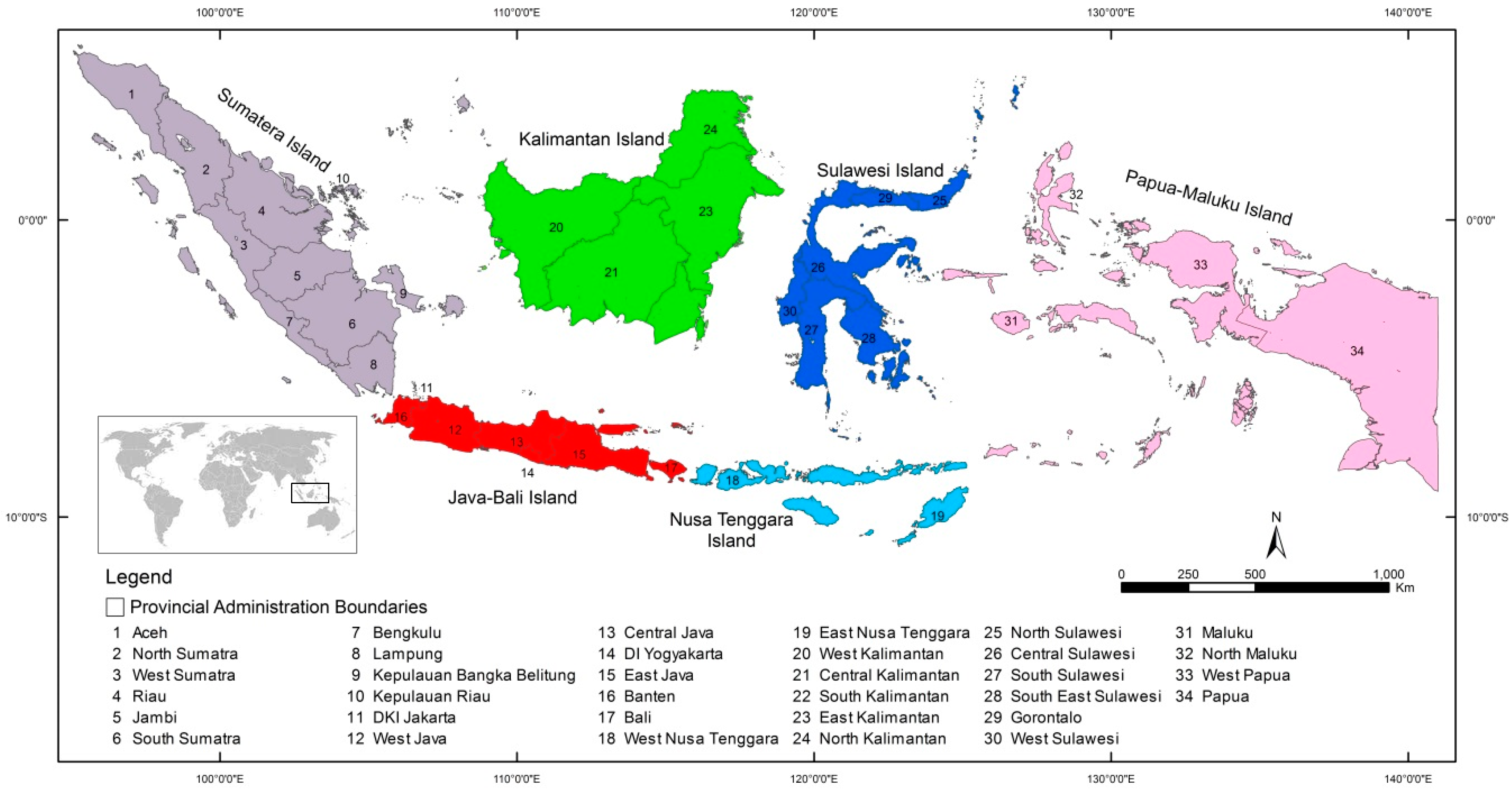
Figure 1. Map of study area: Indonesia.
Sustainability 12 01638 g001
Figure 2. Spatial regression decision process. Source: Adopted from Anselin and Rey [77].
Sustainability 12 01638 g002
Figure 3. Standard deviation map of spatial distribution of (a) food expenditure, (b) urbanization level, (c) economic growth, (d) gross domestic regional product (GDRP) per capita, (e) poverty severity index, and (f) unemployment rate.
Sustainability 12 01638 g003
Figure 4. Global autocorrelation of food expenditure.
Sustainability 12 01638 g004
Figure 5. Local indicators of spatial association (LISA) cluster (a) and significance map (b) of food expenditure. Note: high–high: provinces with high food expenditure surrounded by provinces with high food expenditure. Low–high: provinces having low food expenditure surrounded by provinces with high food expenditure. High–low: provinces with high food expenditure surrounded by provinces with low food expenditure. Low–low: provinces having low food expenditure surrounded by provinces with low food expenditure.
Sustainability 12 01638 g005
Table 1. Ordinary least square estimation of food expenditure.
VariablesCoefficientStd. Errort-Statisticp-Value
Constant63.65073053.130879820.32998240.000
Economic Growth−0.84298510.3422346−2.46317890.020
GDRP per Capita−0.03854590.0204640−1.88359370.070
Poverty Severity Index−0.73347430.9625873−0.76198210.452
Unemployment Rate0.65771120.29634282.21942700.035
Urbanization−0.18066170.0380845−4.74370410.000
R20.6688
Maximized log-likelihood (LIK)−80.354
Akaike information criterion (AIC)172.708
Schwartz criterion (SC)181.866
Table 2. Regression diagnostics.
DFValuep-Value
Multicollinearity condition number: 16.933
Normality of errors (Jarque–Bera test)20.0080.996
Heteroskedasticity random (Breusch–Pagan test) coefficients518.8190.002
Table 3. Diagnostics for spatial regression modelling.
TestMI/DFValuep-Value
Lagrange multiplier (LM)-lag17.5720.006
Robust LM-lag19.6820.002
LM-error (ERR)11.7260.189
Robust LM-ERR13.8360.050
LM-Sarma211.4080.003
Table 4. The results of the spatial lag model of food expenditure.
VariablesCoefficientStd. Errort-Statisticp-Value
Constant76.20774494.116184118.51417300.000
Economic Growth−0.96406380.2675532−3.60325990.000
GDRP per Capita−0.03996120.0159744−2.50157340.012
Poverty Severity Index−3.23157500.9829683−3.28756780.001
Unemployment Rate0.91176490.24092073.78450240.000
Urbanization−0.20660330.0303278−6.81233350.000
W_Food Expenditure−0.20798290.0567949−3.66200000.000
pseudo-R20.7555
LIK−75.306
AIC164.611
SC175.296