Article

Stimulating Implementation of Sustainable Development Goals and Conservation Action: Predicting Future Land Use/Cover Change in Virunga National Park, Congo

by
Mads Christensen
and
Jamal Jokar Arsanjani
*
Geoinformatics Research Group, Department of Planning and Development, Aalborg University Copenhagen, A.C. Meyers Vænge 15, DK-2450 Copenhagen, Denmark
*
Author to whom correspondence should be addressed.
Sustainability 2020, 12(4), 1570; https://doi.org/10.3390/su12041570
Submission received: 7 December 2019 / Revised: 11 February 2020 / Accepted: 12 February 2020 / Published: 19 February 2020

Abstract

:
The United Nations 2030 Agenda for Sustainable Development and the Sustainable Development Goals (SDG’s) presents a roadmap and a concerted platform of action towards achieving sustainable and inclusive development, leaving no one behind, while preventing environmental degradation and loss of natural resources. However, population growth, increased urbanisation, deforestation, and rapid economic development has decidedly modified the surface of the earth, resulting in dramatic land cover changes, which continue to cause significant degradation of environmental attributes. In order to reshape policies and management frameworks conforming to the objectives of the SDG’s, it is paramount to understand the driving mechanisms of land use changes and determine future patterns of change. This study aims to assess and quantify future land cover changes in Virunga National Park in the Democratic Republic of the Congo by simulating a future landscape for the SDG target year of 2030 in order to provide evidence to support data-driven decision-making processes conforming to the requirements of the SDG’s. The study follows six sequential steps: (a) creation of three land cover maps from 2010, 2015 and 2019 derived from satellite images; (b) land change analysis by cross-tabulation of land cover maps; (c) submodel creation and identification of explanatory variables and dataset creation for each variable; (d) calculation of transition potentials of major transitions within the case study area using machine learning algorithms; (e) change quantification and prediction using Markov chain analysis; and (f) prediction of a 2030 land cover. The model was successfully able to simulate future land cover and land use changes and the dynamics conclude that agricultural expansion and urban development is expected to significantly reduce Virunga’s forest and open land areas in the next 11 years. Accessibility in terms of landscape topography and proximity to existing human activities are concluded to be primary drivers of these changes. Drawing on these conclusions, the discussion provides recommendations and reflections on how the predicted future land cover changes can be used to support and underpin policy frameworks towards achieving the SDG’s and the 2030 Agenda for Sustainable Development.

1. Introduction

Established in 1925 as the first National Park (NP) in Africa, the Virunga NP is located in the Albertine Rift Valley in the eastern part of the Democratic Republic of the Congo [1]. Along with the Mgahinga Gorilla NP in Uganda and the Parc Nationale Des Volcans in Rwanda, Virunga is part of a triangle of NP’s in central Africa, principally designated in order to enhance conservation efforts to protect the critically endangered mountain gorilla (Gorilla Beringei Beringei) [2]. The park covers an area of 790,000 ha [3], and hosts the majority of the fragments of the last remaining habitat suitable for the mountain gorilla. Furthermore, the multitude of variety in nature and climate variables, including large lakes, open land savannah, vast forest areas, snow-covered mountain tops and erupting volcanoes, provides critical habitats for a great variety of the other large species of mammals we associate with Africa [1]. For this reason, the park was inscribed as a United Nations (UN) Educational, Scientific and Cultural Organization (UNESCO) World Heritage site in 1979. However, the NP is located in one of the most densely populated regions in sub-Saharan Africa, which has been the scene of prolonged political turmoil and social conflict [4], causing severe pressure on the ecological integrity of the landscape and its biodiversity. Moreover, the rich volcanic soil and high rainfall within the Virunga NP catchment makes it highly suitable for agriculture, and thus an attractive opportunity to underpin subsistence and commercial farming operations [2].
The rapidly increasing population has significantly increased the demand for natural resources (land, water energy, food, etc.), causing rapid land clearing for agriculture and grazing, removal of plants for different purposes, including artisanal mining operations, and house building [4]. Despite the efforts of authorities to protect the integrity of the NP, multiple pressures continue to threaten its habitats and biodiversity, including: civil unrest; illegal activities; land conversion and encroachment; livestock farming / grazing of domesticated animals; widespread depletion of forests in the lowlands and; a massive influx of 1 million refugees occupying adjacent areas of the park [5]. Militia leaders and prospectors are threatening the borders of the park in search for the vast deposits of diamonds, gold, uranium and other coveted minerals, while the vast influx of destitute refugees resorts to poaching and charcoal production, resulting in further fragmentation and degradation of the forest landscape [1]. In fact, the majority of the total population of nearly 6 million people in the surrounding province of North Kivu rely entirely on charcoal for their cooking needs, and an estimated three-quarter of this charcoal is sourced from the Virunga catchment, most of it illicitly from within the NP [6].
Thus, the region is highly important, both ecologically and economically, and the conflicting demands for socioeconomic development while maintaining the ecological integrity of the NP has underpinned the need to ensure continued conservation efforts and sustainable natural resource management. This is critical in order to safeguard the biodiversity and habitats of the NP, while preserving the foundation of the livelihoods of millions of people. This agenda is fortified through the UN 2030 Agenda for Sustainable Development and the 17 Sustainable Development Goals (SDG)’s that were adopted at the UN general assembly in 2015. The SDG’s call on concerted action to pursue economic development while ensuring social inclusion and environmental sustainability on the basis of good governance. The SDG framework provides a comprehensive agenda through which to mainstream policies and derive targeted actions for addressing core sustainability challenges. However, the ability to target policies and actions to address conservation issues, while pursuing economic development and prosperity, leaving no one behind, is hampered by lacking scientific evidence and data to direct and support informed decision making.
In order to derive targeted policies and actions to support effective land use planning, management and ecological restoration conforming to the requirements of the SDG’s, it is imperative to understand the underlying processes of change [7]. Up-to-date information on current land cover and land use provides critical information that can be used to underpin decision-making processes, while modelled predictions about plausible future land use/land cover (LULC) scenarios provide indications of potential trajectories and thus a platform for identifying interventions. Changes in land use and land cover can be described and projected through the use of land change models, which can be used to explain and assess the dynamics of land cover- and broader system change [8]. Spatial land change models thus provide platforms for exploring potential future scenarios, which can be used to guide land use decision making and planning [8].
The purpose of the study is to assess and quantify past and plausible future land use and land cover changes and dynamics within the Virunga case study area. The primary analysis will be guided by a change analysis of classified satellite imagery to quantify past changes, and the development of a land change model, applying a coupled machine learning—the Markov chain approach—to derive a future land cover prediction for the year 2030. The aim is to assess the plausible future evolution of the landscape within the Virunga case study area and address an existing data gap in order to provide evidence to support data-based decision-making processes conforming to the requirements of the SDG’s.

Problem Statement and Research Questions

While several studies have already successfully applied predictive land change modelling to support land use management and decision-making processes [9,10,11,12], a thorough literature review indicates that such an approach has been applied in just a few case studies and hence it is necessary to explore further cases in order to assure its applicability across different landscapes. Therefore, a remote area is targeted in Africa covering the Virunga NP and its immediate vicinity. This study aims to apply remotely sensed data and geospatial and modelling tools to detect, quantify, analyse, and predict future land change in the Virunga NP and its immediate vicinity. Hence, the following research questions are targeted:
  • Have there been major land cover changes within the study area in the last 10 years? And if so, what kind of land cover changes?
  • What has the spatial extent of the land cover change been and which areas have experienced the highest rate of changes?
  • What are the major driving forces behind these changes?
  • What will the extent of land change be by 2030?
  • How can the future land cover prediction for the Virunga study area be used to support and underpin policy frameworks towards achieving the SDG’s?
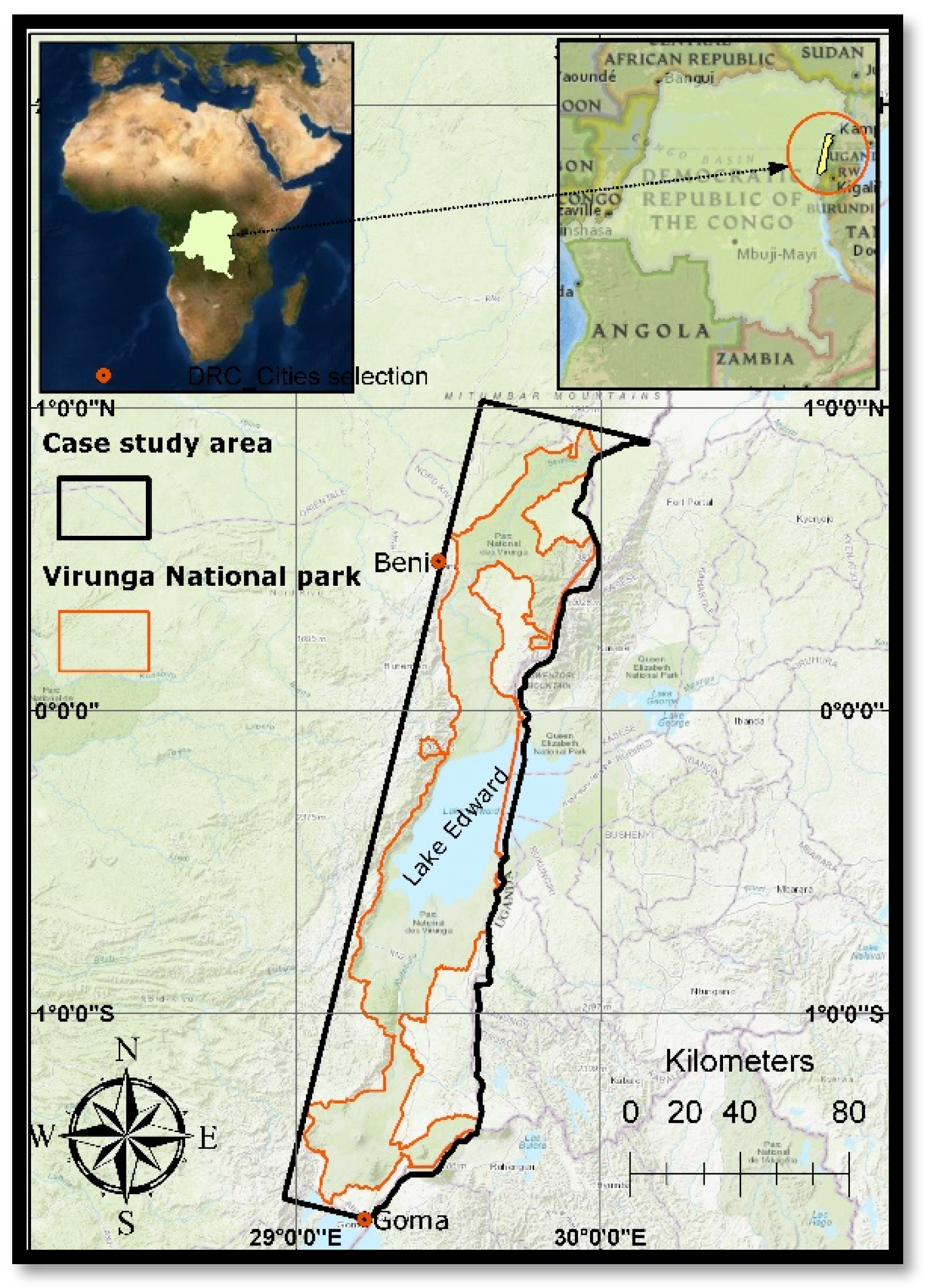
2. Study Area

The Virunga NP is located in Central Africa, in the Eastern part of the Democratic Republic of the Congo, on the border with Uganda and Rwanda. It is located in the equatorial zone, within the Albertine Rift, of the Great African Rift Valley [3]. In this study, The Virunga NP and its immediate vicinity was used as case study area in order to assess the dynamics within the NP and the landscape dynamics of the entire Virunga catchment. The study area is created from a minimum-bounding rectangle encompassing the entire NP, clipped at the Rwandan border. It was considered critical to include the border areas around the NP in order to explore socioeconomic changes, primarily in the form of urban development and cropland expansion, outside of the NP, and assess how these land cover dynamics could potentially impede conservation efforts and sustainable land management planning. The study area, as shown in Figure 1, covers a total of 14,810 km2 of which 7779 km2 is within the Virunga NP.

3. Methodology

The methodological framework utilized in this study to predict the future landscape around the Virunga NP was developed using a variety of different tools and the theoretical framework outlined below. The workflow is illustrated in Figure 2.
In this section, the methodology applied in this study to derive land cover predictions for the year 2030, conforming to this sequential stepwise approach is described. All datasets were either created in, or re-projected to, a Reseau Geodesique de la République Democratique du Congo (RDC) 2005 Transverse Mercator (TM) Zone 18 (EPSG:4051) projected coordinate system, recommended for use in the Democratic Republic of the Congo. ArcGIS was used as a primary tool for data preprocessing and visualisation of results.

3.1. Land Cover Classification

Google Earth Engine provides a cloud-based platform for accessing and processing large amounts of both current and historical satellite imagery, including those acquired by the Landsat-7 and Landsat-8 satellites. The advantages of seamless integration of archived, and pre-processed satellite imagery, along with a powerful cloud-processing platform made Google Earth Engine an ideal platform for conducting the land cover classification. The land classification in Google Earth Engine is composed of several different steps;
  • Choosing an appropriate satellite imagery dataset, fitting the objective of the study,
  • Define land cover classes and collect training data to train the supervised classification algorithm,
  • Developing a JavaScript code to acquire, process and classify the satellite imagery based on the choice of classification algorithm.

3.1.1. Satellite Imagery

In this study, three land cover maps were created, one for 2010, 2015 and 2019. As the National Aeronautics and Space Administration (NASA)’s Landsat satellites provides an archived and freely available dataset covering the entire study period with high resolution (30 m) multispectral imagery, these were selected for this study. Google Earth Engine provides integrated access to analysis-ready (already geometrically corrected and orthorectified), surface reflectance Landsat data from the Tier-1 collection. For the 2010 land cover map, tier-1 data from the Landsat 7 Enhanced Thematic Mappers (ETM+) sensor were selected, while tier-1 data from the Landsat 8 Observation Land Images (OLI) were chosen for the 2015 and 2019 land cover maps. For all three land cover maps, cloud-free composite images were generated from a stack of multiple images collected from the preceding three years (i.e., the 2010 land cover map is based on images from 2008–2010). Only images with less than 30% cloud cover were used in the compositing process, resulting in approximately 60–70 useable tiles for each three-year period.

3.1.2. Collecting Training/Validation Data

As a first step in preparing a training dataset for the land classification, the definition of a nomenclature of land cover classes fitting the objective of the study needed to be defined. Accordingly, the 5 following land cover classes were enough to ensure a sufficient representation of the spatiotemporal variety of land cover changes and identify the primary drivers contributing to forest change dynamics.
  • Forest: afforested and primary forest areas. (Note: While the authors acknowledge the significant difference between afforested areas and primary forest, further separation of the two classes would have caused significant classification errors, due to the spectral similarity of the two classes. Accordingly, the two classes were merged into a combined forest cover class to increase classification accuracy of forest cover.)
  • Water: lakes and rivers.
  • Urban areas: developed residential or industrial areas, roads and urban fringes.
  • Cropland: planted or bare crop fields.
  • Open land/grassland: areas with sparse vegetation, characterized by open grasslands, bare soil or volcanic ash.
To train and validate the land-cover classifications, a reference training dataset was collected within the study area. The minimum samples for machine learning based algorithms to perform optimally should be at least 10 times the number of land cover classes. Thus, the training data samples should be at least 50. These reference training datasets were collected by drawing polygons and clicking points within the Google Earth Engine map interface. The points and polygons were randomly collected throughout the case study area, collecting multiple instances of training data samples for each land cover class. From the collection of training data polygons and points, a subsample of 500 points was used to train the model. An additional point dataset consisting of 50 individually sampled points were collected and used for validation. The validation dataset (i.e., ground truth) was sampled using high-resolution images available in the Google Earth archive from representative years between 2010–2019.

3.1.3. Land Cover Classification within the Google Earth Engine IDE

In order to create the three land cover maps, three individual scripts were prepared within the Google Earth Engine Integrated Development Environment (IDE), one for each of the three years. The JavaScript source code for the land cover classification is included in the Appendix A. The first component of the script was to import the area of interest (AOI) as table data. Secondly, five empty containers for geometry collections for the training datasets were imported as variables. Subsequently, the cloud-free composite of satellite images was imported using the JavaScript code. The function ‘maskClouds’ generates a cloud and a cloud shadow mask for the imported Landsat collection. Furthermore, within this function, the Normalized Difference Vegetation Index (NDVI) was calculated and added to the band collection of the satellite image composite. The NDVI was added to the band collection to enhance the contribution of vegetation in the spectral response for the classification. In addition to NDVI, the first seven bands of the Landsat 8 composite were used in the classification algorithm for the 2015 and 2019 land cover maps. Bands 1-5, band 7 and the added NDVI band were used for the 2010 land cover map, based on the Landsat 7 composite. Thereafter, 500 sample points for each training layer were generated by looping over each training dataset and creating random points within the geometries of the training data layers. Lastly, a confusion matrix was created in order to assess the performance of the classification algorithm.

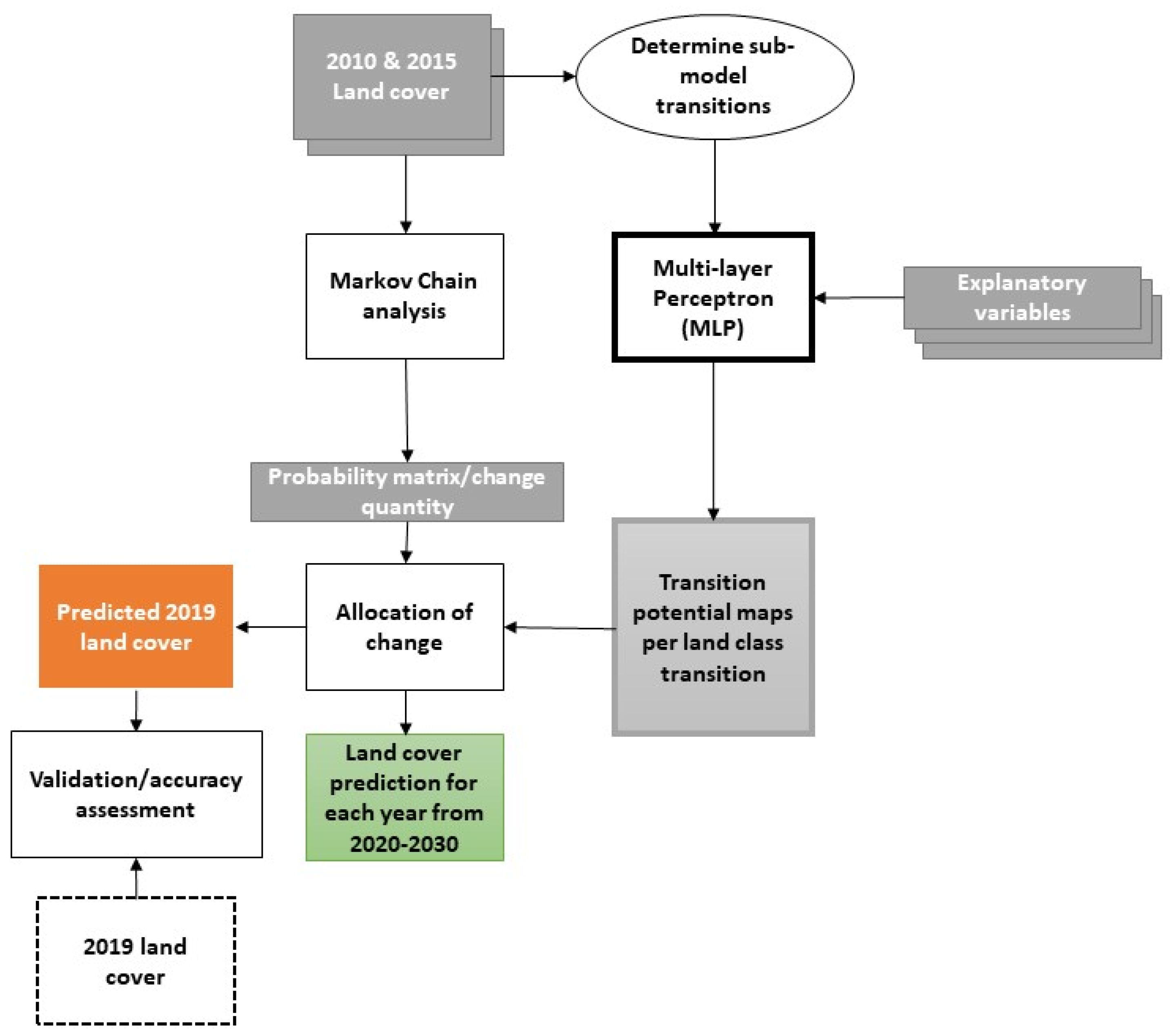
3.2. LULC Modelling and Prediction

The Land Change Module (LCM) within TerrSet (Geospatial Monitoring and Modeling Software) was used to conduct the sequential steps conforming to the requirements of LULC modelling using a multi-layer perceptron (MLP)-Markov chain approach. In this section, each step of the LULC modelling process is described.

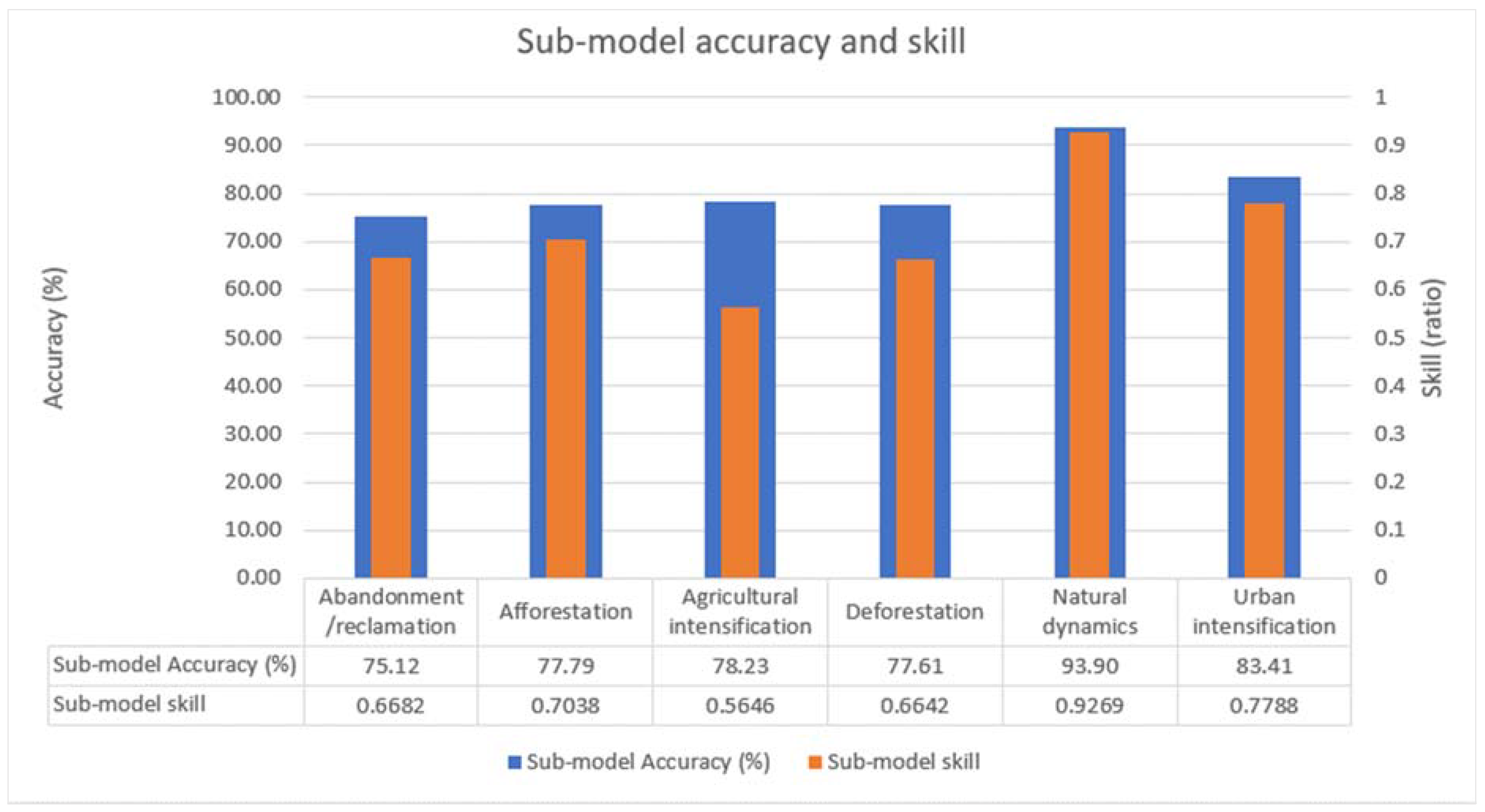
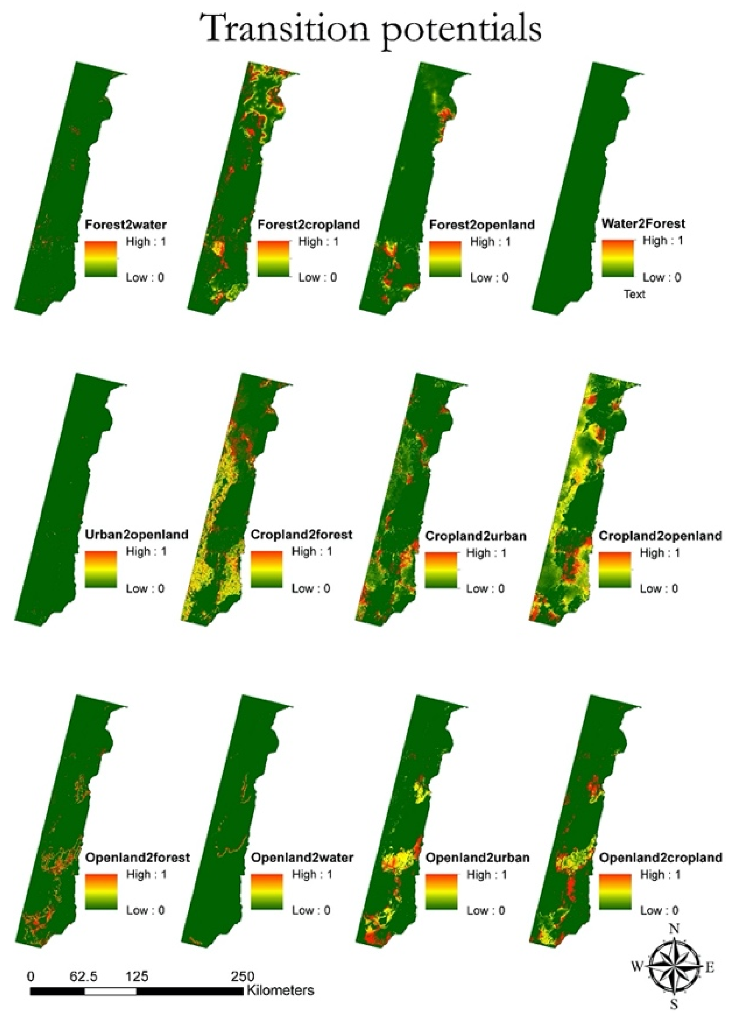
3.2.1. Modelling Transition Potentials: Submodels

The second step in the LULC change prediction process is to model the transition potentials, which are in essence maps of suitability/likelihood of one land cover changing into another [13]. Following [14] the land cover transitions can be grouped together into empirically evaluated transition submodels when the common underlying drivers are assumed to be the same. The submodels can consist from a single land cover transition (e.g., from open land to cropland) or from multiple transitions, grouped together based on the assumption that transitions are caused by the same underlying drivers of change. The explanatory variables are used to model the historical change process based on the empirical relationship between the measured change and the explanatory variable.
Based on the major land class transitions identified in the previous step, the 12 predominant transitions were grouped together based on transition type to form six individual submodels. The composition of transition groups and a description of the types of changes under each submodel can be seen in Table 1. Although persistence, i.e., areas that did not change, can be considered a trajectory, it cannot be considered as a transition class, and thus areas of persistence are ignored in LCM [10].

3.2.2. Explanatory Variables

LULC change processes are dynamic and result from the interaction between a range of different, primarily biophysical and socioeconomic criteria. In LULC change modelling, these criteria are also referred to as ‘explanatory’ variables, as these explain the components of the causal relationships determining the land cover dynamics and they form a critical prerequisite for developing a realistic land change model. The explanatory variables sum up the “knowledge” that the model will use to simulate future land cover scenarios [15]. Each explanatory variable was tested for its potential explanatory value using Cramer’s V scores. Cramer’s V is a coarse statistic measure of the strength of association or dependency between two variables and it ranges from 0.0 to 1.0 in values. Generally, variables with a total Cramer’s V score higher than 0.15 are considered useful and those with a score over 0.4 are considered good [13].
In choosing explanatory variables, the processes contributing to land cover change needs to be visualised in the form of a spatial dataset representing the underlying changes, at a spatial resolution consistent with the land cover maps (30 m). GIS data sets (further described in Table 2) were identified to describe the transitions in the case study area and geoprocessing was performed to derive spatial datasets to, either directly or as a proxy, explain the underlying changes for each transition. According to [16] variables cannot be categorical and thus needs to be continuous and quantitative. The drivers that were used in this study include; elevation (Digital Elevation Model (DEM)), aspect (Asp), slope, Evidence Likelihood (EL), distance from artisanal mines (D_am), distance from disturbance (D_disturb), distance from cities (D_cities), distance from forests (D_forest), distance from mining concessions (D_mining), distance from roads (D_roads), distance from waterways (D_water).
For each land cover class, evidence likelihood answers the question, “How likely is it that you would have this if you were an area that would experience change?” [13], meaning that it established the suitability of each pixel to transform into urban areas or cropland. To do this, evidence likelihood transforms a categorical variable into a continuous surface, based on the relative frequency of pixels belonging to the different categories within the areas of change [17]. In this study, evidence likelihood is a quantitative measure of the frequency of change between urban areas and cropland (also called disturbance) and all other land classes from 2010–2015. Thus, it represents the relative frequency of the different land cover classes that occurred in the areas that transitioned to urban or cropland. This variable aims to explain the geospatial processes that determine urban expansion and agricultural intensification.
The distance drivers represent the proximity of pixels to forces that either constraints or incentivise land cover changes. Mining activities is one of the primary driver of deforestation within the Virunga area “Artisanal mining operations are unregulated and often occur in riparian zones, removing forest and vegetation cover to process the mineral soil.” [18]. Accordingly, there is a documented relationship between deforestation and mining operations, thus, distance from artisanal mines and distance from mining concessions are included as proxy drivers of forest conversion, the rationale being that the closer in proximity a forested area is to known mining operations, the more likely it is to be deforested. Likewise, these drivers will likely positively correlate with an increase of open land, urban areas and cropland nearer to the mining concessions. Distance to disturbance is a spatial driver made from extracting Euclidian distances from areas that were urban or cropland in 2010. The hypothesis is that future anthropogenic disturbance is believed to be closer to areas of existing disturbance, and thus distances to existing disturbances are believed to be closely correlated with urbanisation processes and agricultural expansion.
Table 2 below describes the input datasets as well as the geoprocessing steps of each of the explanatory variables.

3.2.3. Modelling Transition Potential—MLP Calibration

Artificial neural networks are types of computational frameworks for a collection of units or nodes (also called neurons or perceptrons), which aim to mimic the human brain [19]. In this study, an MLP neural network was trained in order to model the nonlinear relationships between land cover change and the explanatory variables, thus deriving the transition potential for each type of land cover change. Operationally, within the LCM, MLP creates a random sample of cells that transitioned and a sample of cells that persisted and use half of the samples to train the model and develop multivariate functions (adjusting the weights) to predict the potential for change based on the value of the conditions at each location [15]. The other half of the subset sample of cells that transitioned and persisted is used to test the performance of the model (validation).
The 12 major transitions which occurred in the period between 2010 and 2015 were grouped together in 6 different submodels, namely; Abandonment/reclamation, Afforestation, Agricultural intensification, Deforestation, Natural dynamics and Urban intensification. The next step in modelling the transition potential was to assign the explanatory variables to each submodel. Variables can be added to the model either as static, meaning that they do not change over time, such as slope, or dynamic, meaning that they do change over time, such as proximity to roads (assuming dynamic road development). Static variables are unchanging over time and express aspects of basic suitability for transitions under consideration, while dynamic variables are time-dependent, such as proximity to existing forest areas or road networks, and are recalculated during the course of a future land cover simulation [13]. In this study DEM, slope, aspect, EL, D_am, D_mining and D_water was used as static variables, while D_disturb, D_cities. D_forests and D_roads were designated as dynamic variables. In contrast to the other distance-related variables, D_am and D_mining are defined as static, under the assumption that the geographic location of the mining operations remain fixed and are not expanding over time.
An iterative approach was used to establish the most appropriate, and accurate, combination of driver variables for each submodel, while avoiding overfitting. Each submodel was fitted with all 11 explanatory drivers to being with, and an iterative approach was used to remove the driver with the least explanatory potential, while assessing the accuracy score and skill level of the model after each iteration. The accuracy score provides a value in percentage that indicates how well the model is able to predict the changes that happened between 2010 and 2015, accounting for both change and persistence. The skill measure compares the number of correct predictions, minus those attributable to random guessing, to that of a hypothetical perfect prediction [10]. Thus, the skill measure provides an indication of how the explanatory drivers will explain past changes. The skill is measured on a scale from −1 to 1, where values less than 0 indicates that the model performs worse than what would be expected by random guessing, 0 indicates that the model performs as well as random guessing while values between 0 and 1 indicates that the performance of the model exceeds what is expected by pure chance.
After each iteration of calibrating individual submodels using MLP, a report about the nature of the model performance is created. This provides critical information on the overall accuracy and skill of the model, the skill measure broken down by component (transition and persistence type) and the explanatory power of each variable. In step 1, the variable with the lowest negative effect on the skill is held constant, and this provides information on the explanatory potential of this variable. If the accuracy and skill of the model don’t decrease by much, when holding the variable constant, this suggests that the variable has little value and can be removed [13]. On each iteration of the calibration of each submodel, the variable with the least explanatory potential was removed until a combination of 5-6 of the variables with the strongest explanatory potential was left under each submodel. Consequently, the final selected variables were loaded into the submodel structure to execute the final iteration of the MLP training.

3.2.4. Change Prediction and Model Validation

Following the transition submodel development, the 12 transition potential maps were used as input in a Markov chain model to simulate future LULC changes (Table 3). The Markov chain determines the amount of change using the earlier and later land cover map along with a pre-specified future year [13]. The Markov module produces a transition probability matrix, which is a matrix that records the probability of each land cover class to change into every other land class category. It also creates a transition areas matrix which is a record of the number of pixels that are expected to change from each land cover class over the specified time frame [13]. Finally, the Markov chain creates a set of conditional probability images which reports the probability of a land cover type to be found at each pixel after the specified prediction date [13]. However, as the matrices only determine the quantity of change, the transition potential (suitability) maps are utilized within the Markov analysis to spatially allocate changes in order to make a land cover prediction for a future year [13].
Consequently, Markov chain analysis was used to make a LULC prediction for 2019 and subsequently validated by using the actual 2019 land cover map for comparison. Yearly recalculation stages were assigned in the model to specify the frequency of which the dynamic variables are recalculated in the model. This means that the D_disturb, D_cities. D_forests and D_roads explanatory variables are updated in the model every year until the prediction year.
Besides visually inspecting how the predicted land cover compare with the actual 2019 land cover map, different Kappa Index of Agreement (KIA) scores was used to assess the overall accuracy of the prediction. The KIA scores can be used to test the agreement between a ‘comparison’ map and a ‘reference map’, both in terms of the quantity of cells in each land cover category and the agreement in terms of location of these cells [13]. The Kappa Standard (Kstandard) is equivalent to kappa and indicates the proportion of correctly assigned pixels versus the proportion that is correct by chance. The Kappa for no information (Kno) indicates the overall agreement between the simulated and reference map [13]. The Kappa for location (Klocation) is a measure of the spatial accuracy in the overall landscape, due to the correct assignment of values in each category between the simulated and reference map [13]. The Kappa for stratum-level location (KlocationStrata) is a measure of the spatial accuracy within preidentified strata, and it indicates how well the grid cells are located within the strata. The combination of Kstandard, Kno, Klocation and KlocationStrata scores allows for a comprehensive assessment of the overall accuracy both in terms of location and quantity. All KIA scores range from 0 to 1 (or 0% to 100%), where 0 indicates that agreement is equal to agreement due to chance and 1 (or 100%) indicates perfect agreement.

4. Results

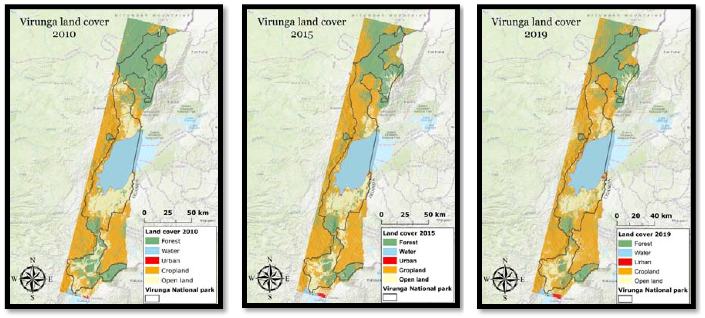
4.1. Land Cover Classification
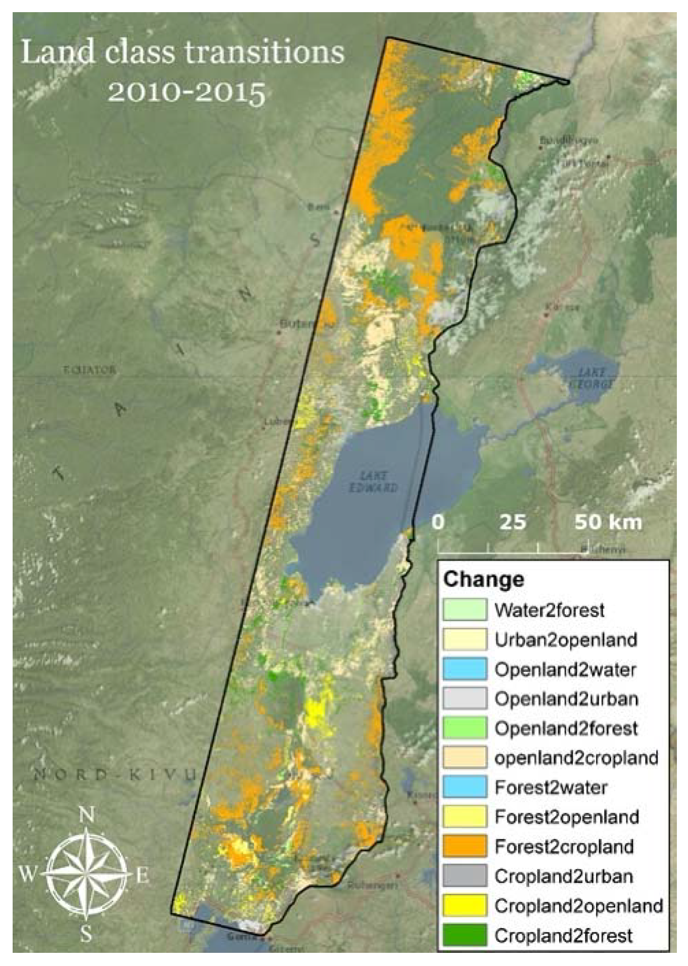
Using the workflow described in Section 3.1, the three land cover maps for 2010, 2015 and 2019 was generated, using Landsat data. The resulting land cover classifications can be seen in Figure 3 below.
The overall accuracy, producers- and users’ accuracy for each of the three land cover maps can be seen in Table 4, and the quantified land cover area under each land class, and for each year, can be seen from the graph presented in Figure 4.

Land Changes

In order to assess the spatiotemporal changes between 2010 and 2015, the earlier and latter land cover maps were cross-tabulated. The cross-tabulation table shown in Table 5 shows the frequencies with which the land classes remained the same (Diagonal) or changed into other categories (off-diagonal frequencies). The table represents quantities of conversion from the earlier to the later land cover data, and it clearly depicts significant changes, primarily between forest and cropland. The following information was obtained about the changes in each class from the table:
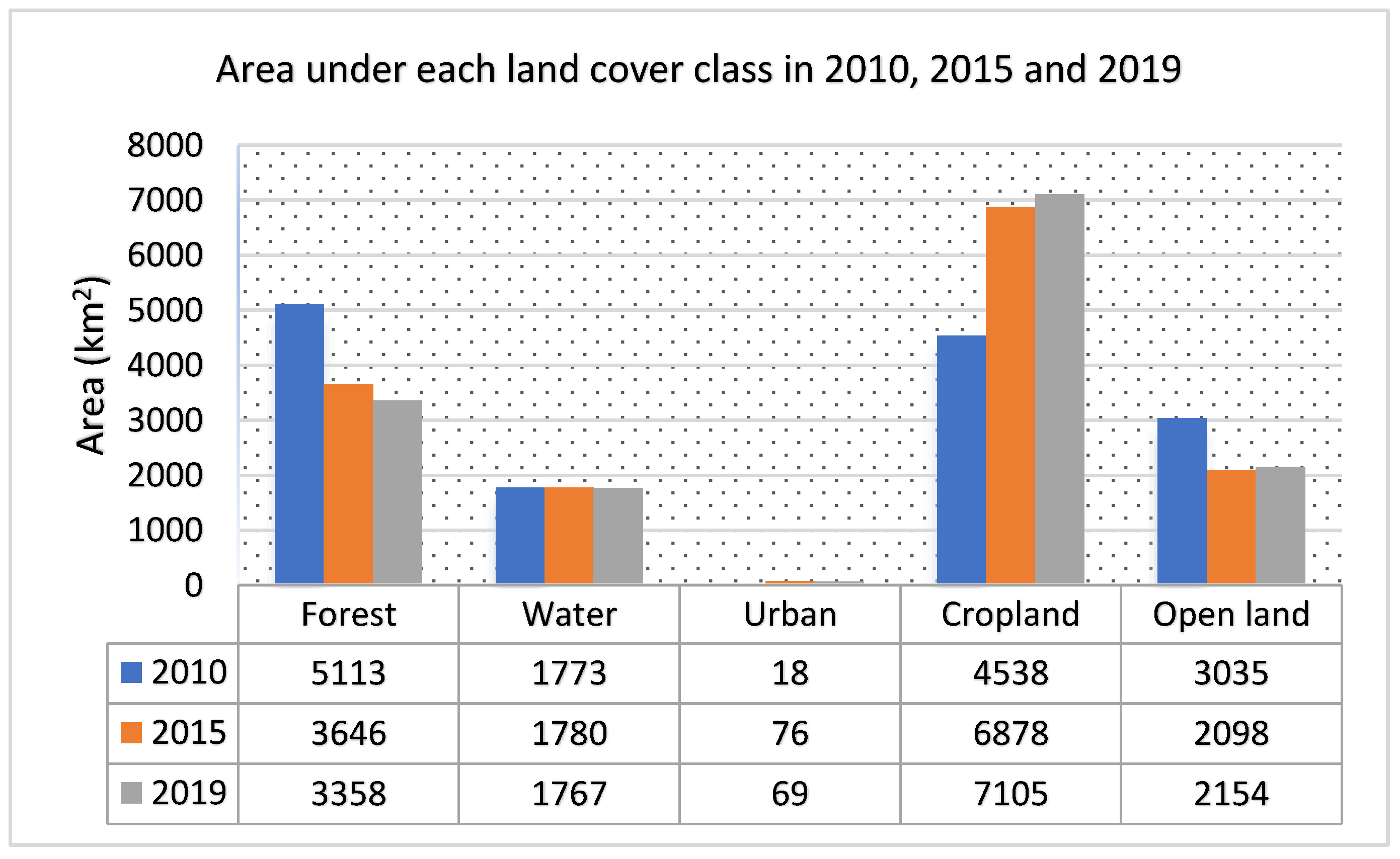
  • Between 2010 and 2015 the forest cover was reduced by 28.7% from 5113.4 km2 in 2010 to 3646.4 km2 in 2015. Even though there was a forest gain of 318.9 km2 largely caused by afforestation from cropland and open land, the net loss of 1467 km2 is almost exclusively attributed to forest conversion into cropland.
  • Accounting for the least prevalent land class in the case study area, urban areas have experienced a large increase between 2010 and 2015, from 17.8 km2 to 75.6 km2, resulting in a 57.9 km2 net gain. This is largely attributed with rapid urbanisation processes in the Democratic Republic of Congo in general, which has an estimated average annual urban population growth rate of 4.3% [20]. The population of the capital city in the North Kivu province, Goma, located in the south-eastern corner of the case study area, increased from 150,000 people in 1990 to more than one million in 2017 [6]. Thus, the majority of the urban class increase is caused by the expansion of Goma.
  • Cropland is the most dynamic land class in the case study area and represents the most dominant land cover type. The total area under cultivation increased by 51.5%, from 4538.4 km2 in 2010 to 6877.6 km2 in 2015. As mentioned previously, cropland is the main driver of deforestation and thus the majority of the agricultural expansion is caused by forest conversion. However, another 47% of cropland expansion is attributed with the cultivation of previously open land/grassland areas.
  • The open land cover class was reduced by 30.8%, from 3035.0 km2 in 2010 to 2098.3 km2 in 2015. Even though the open land class received a total net loss, 236.2 km2 was gained, caused by agricultural abandonment. Another 66 km2 gain of open land is attributed to deforestation. The majority of the net loss of the open land class (1109.2 km2) is associated with agricultural expansion, while another 59,5 km2 is attributed to urbanisation processes. A net loss of 69.8 km2 is associated with afforestation processes.
  • The water bodies remained largely unchanged, which is to be expected as there has been no waterworks (e.g., dam construction) in the study period. Thus, the water bodies, largely consisting from the two major lakes in the study area, Lake Édouard and Lake Kivu, have remained relatively consistent.
The spatial trends of the changes outlined above are illustrated in Figure 5 below.

4.2. LULC Model

Using the 2010 and 2015 land cover maps and the explanatory variables as input data, the model described in the methods section was trained to make a land cover prediction for each year between 2020 and 2030. Table 6 provides a list of the Cramer’s V scores of each explanatory variable used in the model and Figure 6 illustrates all the processed variables.
Table 7 below provides information on the accuracy and skill measure of the model when holding one or more variables constant. This relationship was used to identify the explanatory variables with the strongest explanation potential for each transition type.
The final skill measure and accuracy rate of each model calculated through MLP is summarized in Figure 7 and the explanatory drivers used under each submodel and selected performance scores is provided in Table 8.
The accuracy and skill measure reveal some disparity between the level of confidence of the transition modelling under each submodel, however overall the values are fairly consistent, ranging from 75% to 93%. Abandonment/reclamation has the lowest accuracy score (75.12%), followed by deforestation (77.61%), afforestation (77.79%) and agricultural intensification (78.23%). Agricultural intensification, however, has the lowest skill measure of all the submodels (0.56). Natural dynamics and urban intensification performed best, with accuracies of 93.90% and 83.41%, respectively. The skill measure of these two submodels was also the highest among all six, with 0.93 for natural dynamics and 0.78 for urban intensification. The outcome of the transition potential modelling is a series of transition potential maps, describing the suitability for each of the 12 major transitions included in the submodels. These maps can be seen in Figure 8.

4.2.1. Validating Results

Figure 9 below shows the actual and the predicted land cover map for 2019. The actual 2019 land cover map was created using Landsat data composites from the years 2017–2019, applying the process described in Section 3.1.3. A visual inspection indicates that the predicted land cover map, overall, looks fairly similar to the actual land cover map, however there are localised discrepancies where the model failed to predict changes/persistence, for example, in the mid-west where the simulation predicted cropland to replace large open land areas, when in actuality it did not.
K scores was used to comprehensively assess how the simulated 2019 land cover map ‘comparison’ compare with the actual 2019 land cover map ‘reference’. The K scores are provided in Table 9.
The statistics from the k scores shows that Kno is 0.9224, Klocation is 0.9001, KlocationStrata is 0.9001 and the overall Kstandard is 0.8828. According to [21], a model is valid if the overall Kappa (Kstandard) score exceeds 70% (or 0.7). The Kstandard score, close to 90%, is a very strong indicator of the overall accuracy and performance of the model, and the remaining k scores, all exceeding 85%, indicate that there are almost no, or very small quantification and location errors between the predicted and the actual land cover map for 2019. Thus, the simulation has a strong ability to predict both the quantity and the locations of change.

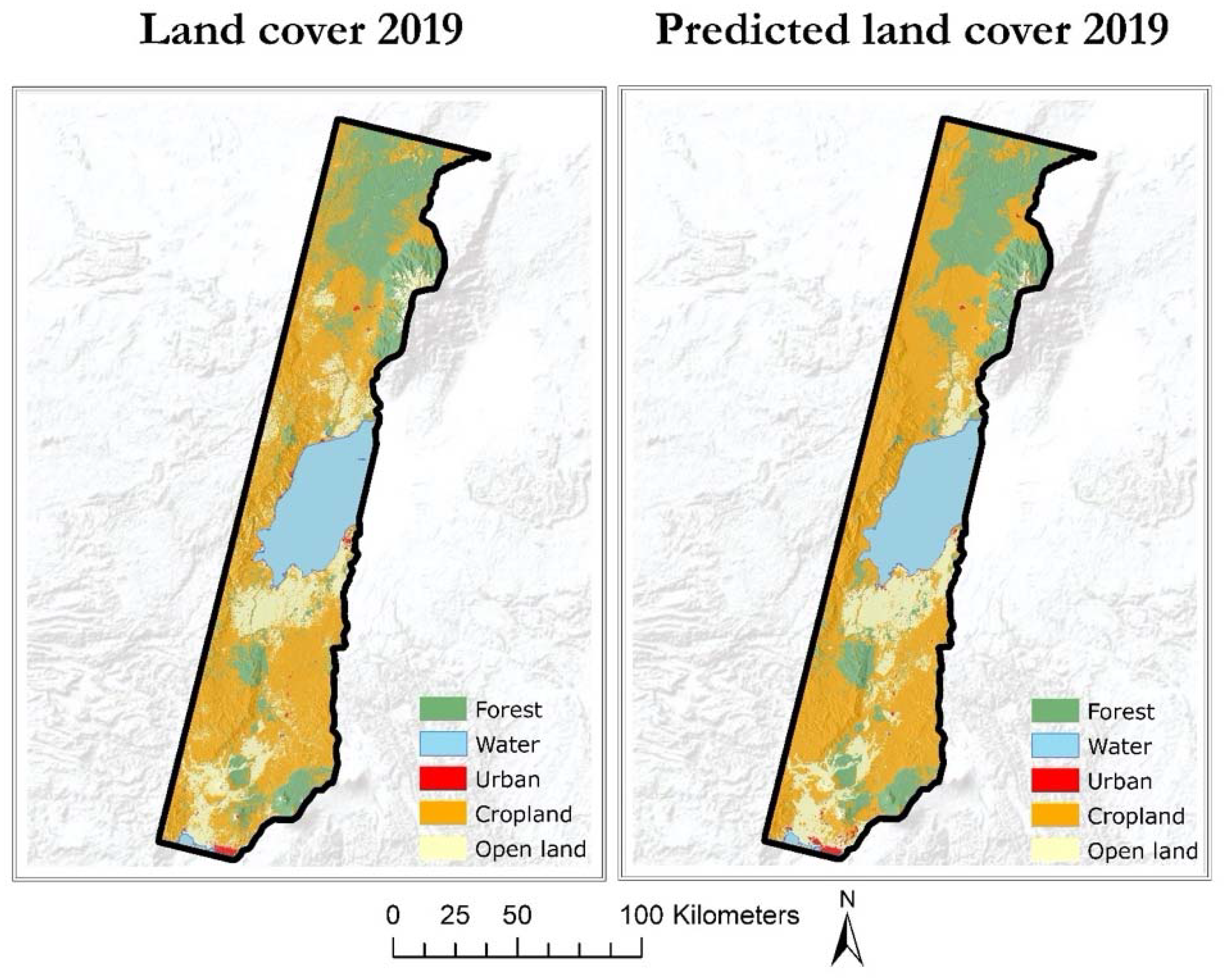
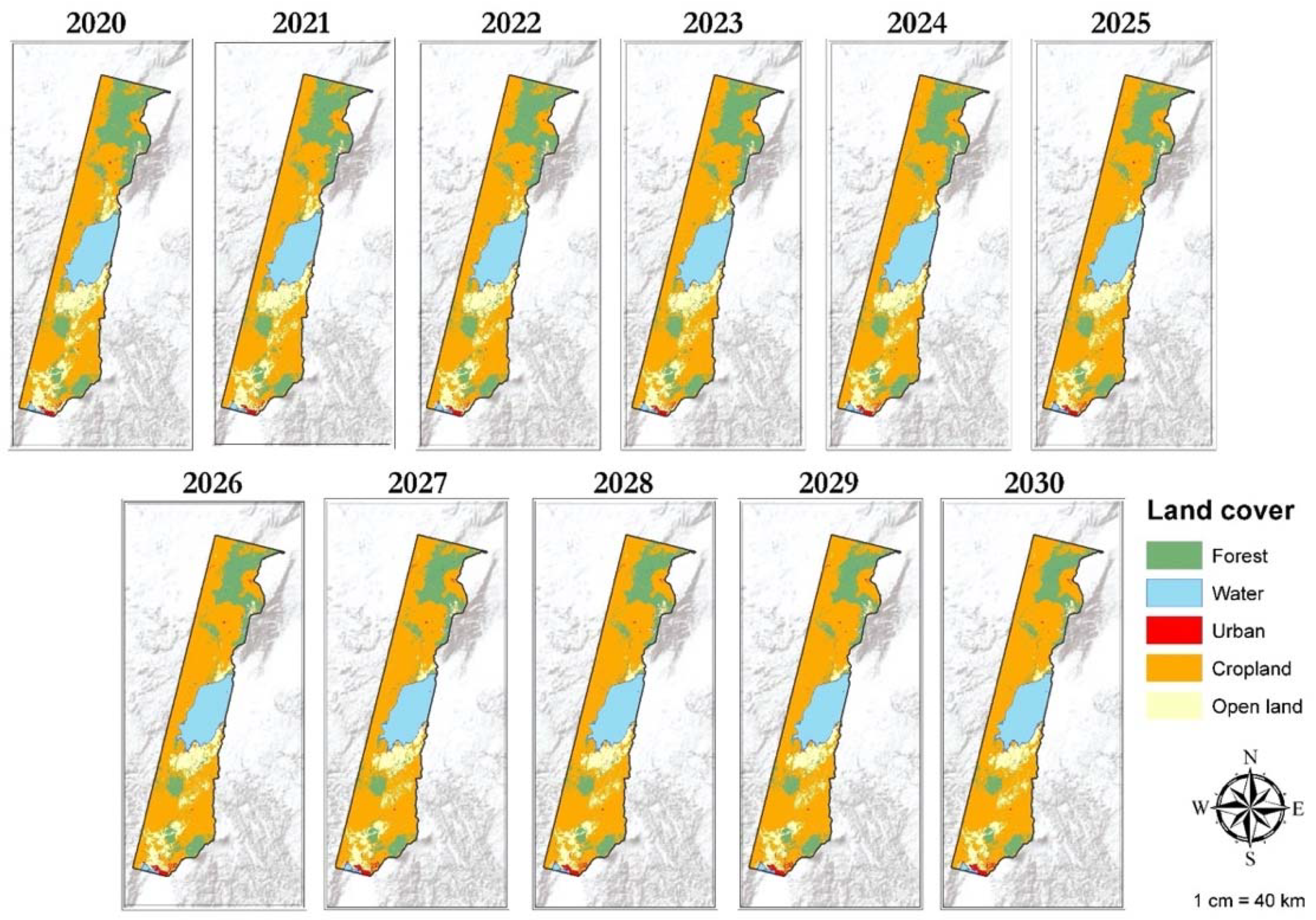
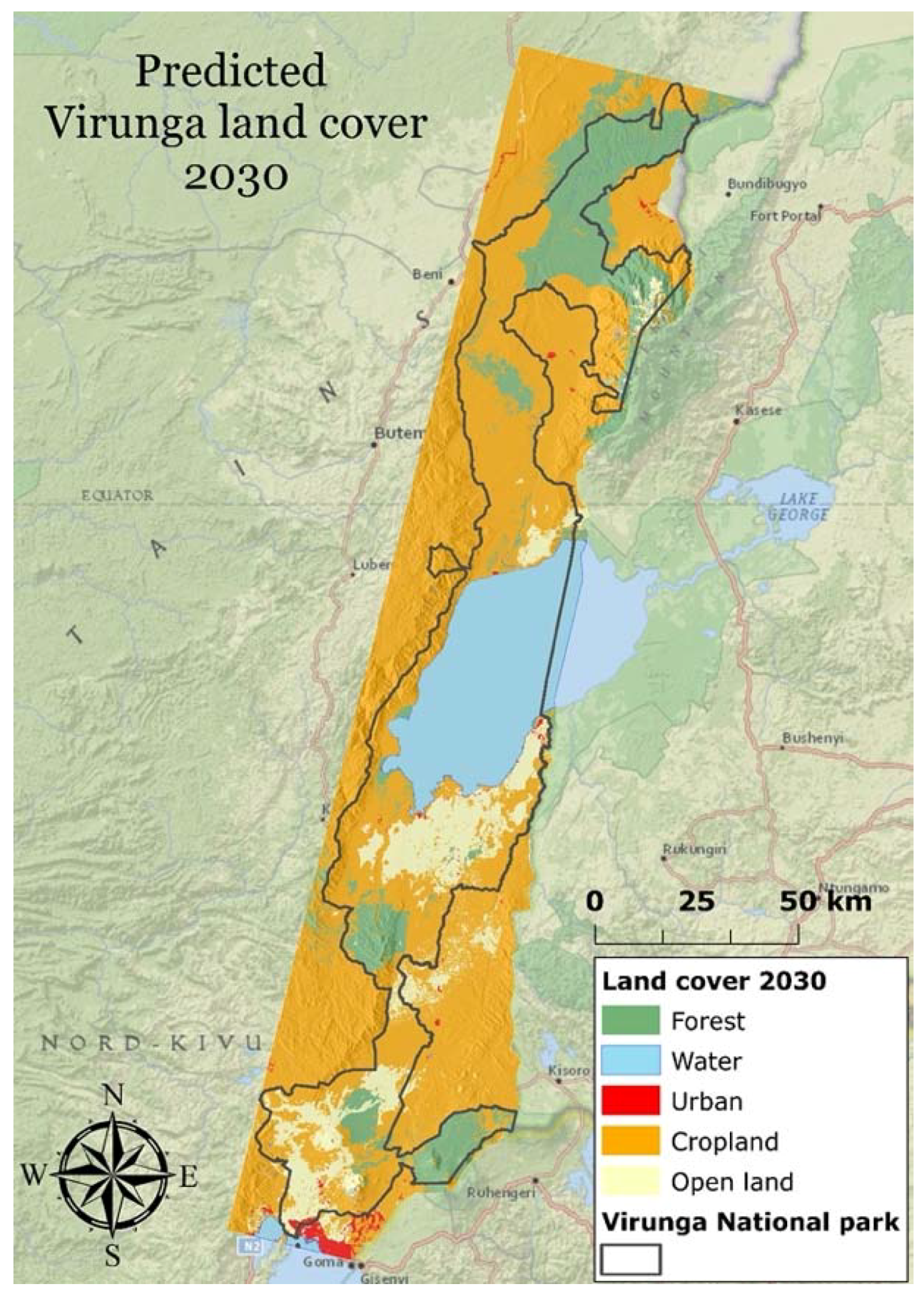
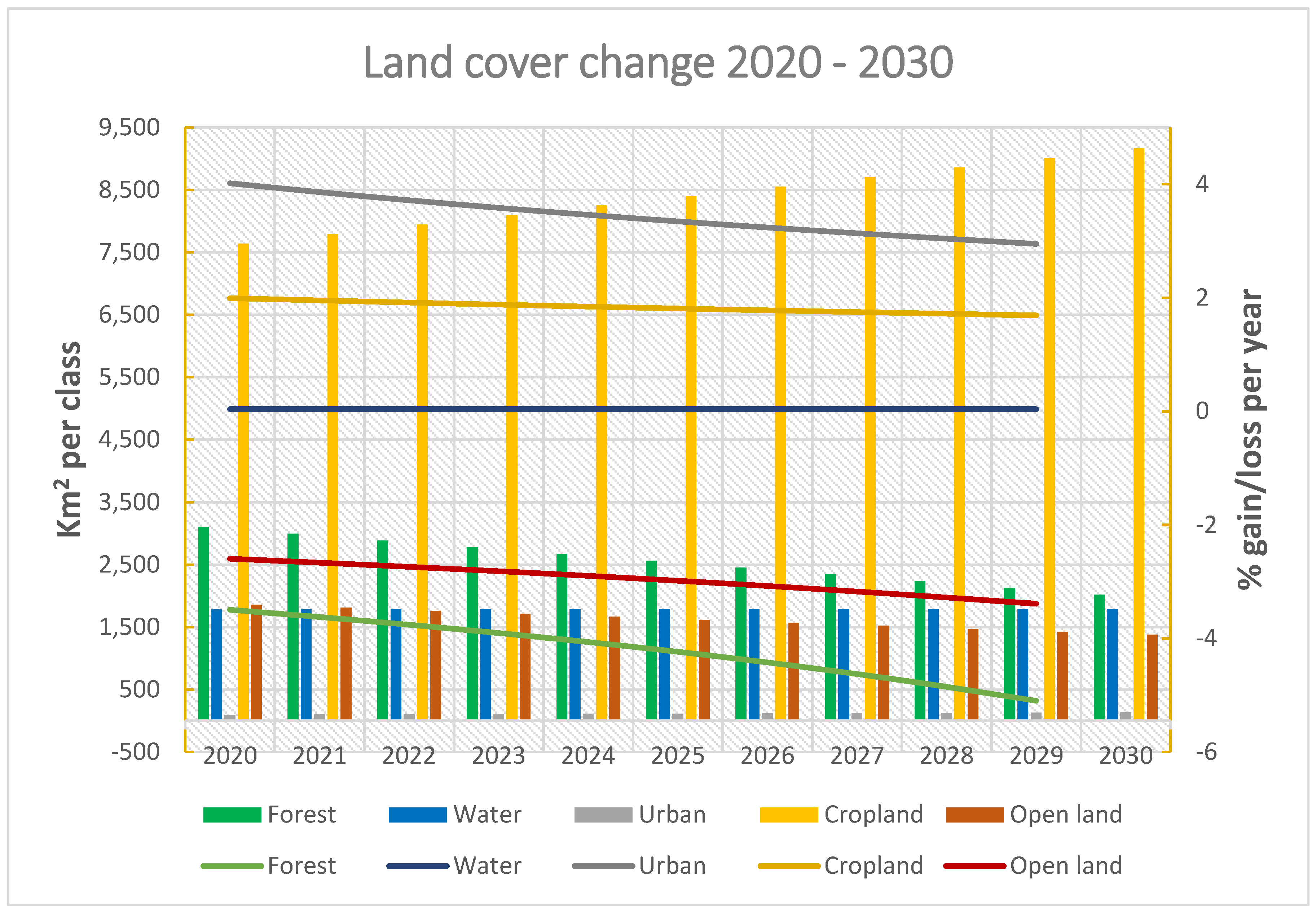
4.2.2. Land Cover Prediction

The resulting compilation of land cover predictions from 2020 through to 2030 can be seen from Figure 10, while the predicted land cover for 2030 is presented in Figure 11.
The series of land cover predictions covering 2020 to 2030, and the final land cover map for 2030 presented in Figure 11 clearly illustrates that the model predicts continuous cropland expansion, primarily at the expense of forest areas and existing open lands. The model also predicts continuous urban development, particularly around existing settlements. The collective change per class in total, and percent change per year, is illustrated in Figure 12. As depicted in the graph, the forest cover will continue to decrease throughout the 10-year period, with an average annual loss of 4.21% and a total area loss of 1085 km2, from 3104 km2 in 2020 to 2019 km2 in 2030. Water coverage will, as expected, remain largely the same, gaining a negligible average of 0.04% per year. Urban expansion and development of new settlements will continue, gaining an average annual of 3.44%. The total urban area is predicted to increase by 38 km2, from 95 km2 in 2020 to 133 km2 in 2030, and looking at the predicted land cover map, most of this is expected to be as a result of urban sprawl around the main city of Goma in south-eastern Virunga. As also visually apparent, cropland expansion will continue throughout the 10-year period, gaining an average annual area of 1.83%, and a total area gain of 1522 km2, from 7636 km2 to 9161 km2 class coverage. Along with forest areas, open land/grassland zones are expected to decrease the most, by 2.96% per year, losing a total of 482 km2 in the 10-year period, from 1857 km2 in 2020 to 1375 km2 in 2030.

5. Discussion

Understanding LULC changes, transitions, landscape risks and dynamics is paramount in order to inform policies, planning interventions and actions aiming to ensure sustainable development in all dimensions (economic, social and environmental) conforming to the objective of the UN SDG’s and the 2030 agenda for sustainable development. In this study, a combined MLP-Markov chain approach has been used to simulate future land cover changes in the period from 2020 to 2030, in a case study area covering the Virunga NP in the Democratic Republic of the Congo and its immediate vicinity. Two simulations were carried out. The first (2019) was used for model validation and accuracy assessment, and the second (2030) was used to predict landscape change within the case study area covering the Virunga NP catchment. The assessment of the spatial patterns of LULC change derived through a change analysis of historical trends combined with the development of a plausible future land cover scenario for the Virunga catchment will help to improve the understanding of the land system and establish cause-effect relationships between driver variables and land cover dynamics. Thus, the LULC change model aims to contribute to informing policy responses aiming to support sustainable land management and landscape planning decisions within the Virunga NP. It aims to provide a blueprint for quantified policy responses aiming to address existing challenges. Follow-up research should aim at applying the LULC model developed for this study for scenario-based analysis of policy response impacts.
As formerly mentioned, the LULC model developed in this study predicts a future land cover state, based on a business as usual scenario. Past land cover changes within the Virunga catchment has been largely linked with charcoal production and cropland expansion, which have impeded conservation efforts and put critical pressure on the ecological integrity of the landscape and its biodiversity. By cross-tabulating two land cover maps for 2010 and 2015, this study aimed to quantify past land cover changes and identify spatial trends of change. It concludes that forest conversion into cropland is the most common and frequent type of landcover change, contributing to the majority of the total net forest loss of 28.7% between 2010 and 2015. The most significant forest loss occurred around the perimeter of the forest areas in the northern sector of the case study area, however, the forest areas just north of the North Kivu provincial capital of Goma, also experienced substantial losses. While a 318.9 km2 forest cover gain was also identified in the change assessment, these gains cannot be qualified in existing literature, and as these gains are largely located within, or close by, existing cropland areas, they may likely be the result of misclassified pixels, possibly classifying plantation development as forest. While the urban cover is the least predominant land class type within the case study area, the cross-tabulation indicated that the urban land cover quadrupled between 2010 and 2015. The majority of the urban gain, however, is associated with significant urban development around Goma, located in the southeastern corner of the case study area. Another major land cover change results from the conversion of open land/grassland areas into cropland. In total, open land areas were reduced by 30.8% in the period from 2010 to 2015 and the majority of these transitions were located just north of Lake Edward.
If unchecked and unregulated, the LULC change model developed in this study indicates that the landscape within and outside the NP will continue to change dramatically in the next 10 years. While Figure 12 in the previous section quantified the collective amount of changes, per land class per year, from 2020 to 2030, Table 10 below quantifies the projected land changes from 2019 to 2030, between land classes. As can be seen from the cross tabulation, forests are attributed with the most significant land class loss in the period from 2019-2030, and almost all forest loss (1579.5 km2 of a total of 1651.1 km2) is associated with cropland expansion. Open land is also projected to experience significant land class loss (1162.8 km2) the majority of which (1081.8 km2) is also attributed to cropland expansion. While urban areas are projected to continue to be the minority land class in the Virunga NP catchment, the total urban area cover is projected to almost double, from 68,5 km2 to 132,7 km2 in the 11-year period. Most of this is attributed to the conversion of cropland and open land areas. Thus, the majority of all transitions, gains and losses, are for the most part attributed with the expansion of agricultural lands, and largely at the expense of forest areas.
Addressing forest loss is a primary component of conservation efforts and land management planning within the Virunga NP catchment. Therefore, it is critical to determine not just the amount of forest cover loss, but also the spatial extent and location of forest dynamics. Figure 13 below illustrates the spatial location of the dynamics of forest land, and as seen from the figure, forest loss is largely concentrated in the northern part of the study area, and particularly the north-eastern margin of the NP. This change is consistent with past deforestation patterns, which has historically been more predominant in the north where larger and more remote forest areas are located, and literature (i.e., [22]) indicate that illegal slashing of old growth forest to produce carbonized wood has been particularly predominant in the northern sector. This is largely caused by rebel groups operating near the city of Beni, supplying local villages and larger cities in the outskirts of the national park with charcoal [22]. Besides charcoal, army groups have also been known to transport illegal timber along the Kamango Route, linking the Democratic Republic of the Congo with Uganda, causing further forest loss and fragmentation [22]. Conversion of cleared forest areas and slashing of trees to plant subsistence crops, such as cassava and maize, is another primary driver of forest loss, particularly in the south [22]. While forest loss is also expected to continue in the southern part of the NP, particularly just north of Goma, the high montane forests to the northeast of Goma is predicted to remain largely intact, likely protected by its high altitude and steep terrain, making the area less accessible and thus less likely to be logged.

5.1. Policy Response Options, Planning Interventions and SDG Implementation

As the LULC change model developed in the context of this study is an empirical-statistical projection of past changes into the future, the outcome represents likely LULC changes as a reflection of a business as usual scenario. Thus, the results help to understand and illustrate how the intrinsic drivers of change will continue to drive land cover changes, if unchecked, while providing valuable information on possible future LULC configurations in the Virunga catchment and thus an indication of the causes and consequences of land-use change. In the absence of reformed regulatory policies, legal frameworks and planning interventions, Virunga NP will continue to be threatened by encroachment and deforestation, primarily caused by cropland expansion and persistent conflict. The high population density and a continuous population growth believed to be around 3% in the Virunga region [2], will inevitably result in fewer resources outside the Virunga NP, which will ultimately put more pressure within the park, resulting in further damaging human impact. The large-scale deforestation and conversion to agriculture caused by human activities will severely alter the integrity of the landscape and cause strong negative impacts on biodiversity and soil degradation, while undermining the natural resource foundation on which the local livelihoods depend. The formulation of adequate spatial policies in the Virunga catchment must balance the competing needs for land to feed the accelerating population and provide energy and resources, while reducing the loss of ecosystems and biodiversity. The SDGs provide the blueprint for such policy planning and interventions, aiming to balance prosperity for both people and the planet.
The direct exploitation of resources and expansion of cropland activities is intimately linked with the economic situation of the people [2], and thus in order to protect the biodiversity and integrity of the Virunga NP, policies should aim to improve and strengthen the economic security and livelihoods of the people living in its vicinity. The Virunga NP exists between the extremes of economic poverty and natural wealth, which has made it a target for all of those who aim to profit from its resources. A 2013 report by the World Wildlife Fund (WWF) entitled ‘The economic value of Virunga national park’ concluded that the “direct use of Virunga’s ecosystem could generate US$348 million per year and help diversify DRC’s economy [23]”. The main direct contributors to this value are tourism (US$235 million), fisheries (US$90 million) and hydropower (US$10 million), while another US$63.8 million, primarily attributed to carbon sequestration and erosion control, can be generated through the provision of ecosystem services [23]. If sustainably managed, the outstanding natural value of the Virunga NP could contribute significantly to the local economy, while providing livelihoods for 45.000 people through the provision of job opportunities [23]. Thus, policies should aim to strengthen conservation action by creating an alternative economy that incorporates and enables the surrounding communities from a thriving and well managed national park, while embracing the framework of the SDGs.

5.1.1. Incentivising Alternatives to Charcoal

As mentioned previously, the vast deforestation in the northern and southern sectors of the park, visualized in the simulated 2030 LULC map, is largely believed to be a reflection of illegal charcoal production and land clearing for agricultural expansion. The major demand for charcoal is located within the major villages, refugee camps and the capital city of Goma in particular. As the majority of the population in Goma rely on charcoal for their entire energy consumption, the prediction of a total clearing of the forest just north of Goma is highly probable and inherently linked with charcoal production and cropland expansion. Electricity is recognized to have substantial benefits for poverty reduction, health and education, and thus access to electricity should be incentivised and subsidized. Realising the US$10 million potential of hydropower in Virunga NP alone, could potentially contribute to provide job opportunities and tax revenue, and more importantly, if sustainably planned and implemented, release pressure on forests to obtain charcoal. Furthermore, the affordability and availability of modern cooking fuels and practices could be subsidised through regulatory reforms, i.e., reducing costs on kerosene stoves and cylinders [24], or through the establishment of microcredit systems. As evident from the LULC change model cropland expansion cause the majority of the land transformation and will continue to grow. Thus, adopting measures to support the development of sustainable biomass production initiatives, i.e., by improving linkages to agriculture, animal husbandry, agroforestry, etc. could be another approach to reduce the dependency on charcoal. Such policy initiatives would not only contribute to promote conservation action, and thus contribute to realizing SDG 15 (Life on land), but also contribute to the realisation of multiple SDG’s, including SDG 1 (No poverty), SDG 3 (Good health and well-being), SDG 8 (Decent work and economic growth), SDG 13 (Climate action) and SDG 7 which aims to ensure access to affordable, reliable, sustainable and modern energy for all.

5.1.2. Community Development

Land grabbing for subsistence agriculture has been another primary driver of change, historically, and unregulated and illegal encroachment has threatened the fringes of the Virunga NP. The LULC change model predicts that vast expanses of the NP will be subject to cropland expansion, at the expense of forests, savannahs and grassland, in 2030. To counteract the infringement, enforcement of existing legislation needs to be strengthened while at the same time community development efforts should aim to build capacity to pave the way for an alternative, and more sustainable, livelihood options for the increasing population [23]. Community-based planning and management is undoubtedly a cornerstone of conservation action and SDG implementation, as local communities are effectively custodians of their environment. Consequently, the local communities should be involved in the wider planning framework in order to maximise the development potential and environmental benefits. Thus, in order to contribute to the conservation of the NP and reduce land grabbing, economic development in the region, communal development projects and community involvement should be promoted, e.g., expanding the fragmented and desolate road infrastructure in order to improve market access, and thus increase revenue potential from agricultural and artisanal productions. Other communal development projects could support the promotion of alternative income generating activities, such as ecotourism development or educational programmes which could facilitate access to the tourism industry, such as free public park ranger or guide training programmes. Depending on the nature of community development programmes, successful implementation of initiatives such as those outlined above could potentially contribute to the realisation of SDG 1 (No poverty), SDG 3 (Good health and well-being), SDG 4 (Quality education), SDG 8 (Decent work and economic growth), SDG 9 (Industry, Innovation and Infrastructure), SDG 11 (Sustainable cities and communities) and SDG 15 (Life on land).

5.1.3. Utilising the LULC Change Model to Gain Intergovernmental Support and Mobilise Resources

While underpinning the need for reformative action to counteract the impact of deforestation and land degradation in Virunga, it is vital to realize that the majority of the policies and actions suggested will require significant investments. Accordingly, the Democratic Republic of the Congo will, to some extent, be relying on support and engagement from donor countries in order to forge strong bilateral relationships through which investments can be sourced and policies framed. Furthermore, collective international support can be forged using the framework of existing Multilateral Environmental Agreements (MEA)’s in order to better integrate conflict-concerns into the implementation and priorities and attain earmarked funding for targeted capacity building and conservation activities. For this purpose, the LULC change model and the simulated land cover for 2030 is not only an effective policy support tool to inform spatial planning and policy-making, but also a vital instrument which can be used for lobbying activities in order to gather support for conservation and poverty reduction activities and strategies at the intergovernmental level. Insight into a probable future LULC scenario within one of the most biodiverse world heritage sites in the world, which indicates that most of the forest resources within the NP will be gone by 2030, may provide further traction to support collective action and mobilisation of resources to preserve the integrity of the park and the biodiversity within it. The fortification of these bilateral and multilateral relationships will be vital in order to mainstream and finance conservation actions across sectoral policies, contributing to sustainable energy production, poverty reduction, education, health etc., thus underpinning a coordinated strategy providing political and economic governance while increasing human capacity and wellbeing. While potentially contributing to realise the majority of the SDG’s, development and revitalisation of global partnerships to strengthen the implementation of the SDG’s is the overall objective of SDG 17 (Partnerships for the Goals).

6. Conclusions

The Virunga catchment in the eastern part of the Democratic Republic of the Congo is subject to dramatic deforestation rates and land grabbing, causing significant changes to the land cover dynamics in one of the most biodiverse regions of Africa. In order to inform conservation actions and management practices to protect the diversity and integrity of the Virunga NP, while developing sustainable land managing policies and socioeconomic reforms it is vital to understand the drivers and dynamics of LULC changes.
This study was successfully able to use a combination of cloud processing platforms (Google Earth Engine), GIS software (ArcGIS) and LULC modelling tools (LCM in TerrSet) to simulate future deforestation and land change patterns in the Virunga catchment. It provides a good understanding of the predicted LULC changes, under a business-as-usual scenario, over the next ten years, and thus presents an effective policy support tool for decision makers and administrative bodies aiming to strengthen SDG implementation while preserving park resources.
The LULC model predicted that the largest shift between classes is attributed with the conversion of forest areas into cropland and the overall general trend is a significant increase in cropland with a net gain of more than 2000 km2. The increase in cropland is primarily located in the north of the Virunga catchment where a substantial proportion of the remaining forest areas is predicted to be replaced by cropland. The primary drivers of deforestation were identified as distance to artisanal mines and mining concessions and distance to cropland and cities, distance to roads and distance to water. These drivers all reflect the inherent relationship between accessibility to forested areas and proximity to human activities, which is consistent with literature and consistent with the hypothesis that charcoal production and land clearing for mining, urban expansion and subsistence agriculture are the primary contributors to deforestation within the Virunga NP.

Author Contributions

M.C. conducted the study, drafted and revised the paper. J.J.A. co-designed the paper and supervised the paper. All authors have read and agreed to the published version of the manuscript.

Funding

This research received no external funding.

Conflicts of Interest

The authors declare no conflicts of interest.

Appendix A

Source code for the 2019 land cover classification in Google Earth Engine
Map.centerObject(AOI, 9);
Map.addLayer(AOI, {}, ’aoi’);
//For Landsat surface reflectance product cloud masking
function maskclouds(image) {
var cloudShadowBitMask = 1 << 3;  // cloud shadow
var cloudsBitMask = 1 << 5;     // cloud
var qa = image.select(’pixel_qa’);
var date = image.get(’system:time_start’);
var mask = qa.bitwiseAnd(cloudShadowBitMask).eq(0)
   .and(qa.bitwiseAnd(cloudsBitMask).eq(0));
var ndvi = image.normalizedDifference([’B5’,’B4’]).multiply(10000).rename(’NDVI’);
return image.addBands(ndvi).updateMask(mask).divide(10000).set(’system:time_start’,date);
}
//Landsat 8 image collection
var L8collection = ee.ImageCollection(’LANDSAT/LC08/C01/T1_SR’)
          .filterDate(’2017-01-01’, ’2019-03-23’)
          .filterBounds(AOI)
          .filter(ee.Filter.lt(’CLOUD_COVER’, 35))
          .map(maskclouds);
print (L8collection);
var testimage = L8collection.median().clip(AOI);
 
Map.addLayer(testimage.select([’B5’, ’B4’, ’B3’]), {min:0, max:0.4}, ’false color’);
Map.addLayer(testimage.select([’B4’, ’B3’, ’B2’]), {min:0, max:0.4}, ’true color color’);
// Subsample training polygons with random points
// this ensures all classes have same sample size
// also EE can’t handle too many cells at once
var trainingLayers = [forest, water, city, cropland, openland2];
var n = 500;
// loop over training layers
for (var i = 0; i < trainingLayers.length; i++) {
 // sample points within training polygons
var pts = ee.FeatureCollection
  .randomPoints(trainingLayers[i].geometry(), n);
 // add class
var thisClass = trainingLayers[i].get(’class’);
 pts = pts.map(function(f) {
  return f.set({class: thisClass});
});
 // extract raster cell values
var training = testimage.sampleRegions(pts, [’class’], 30);
 // combine trainging regions together
if (i === 0) {
  var trainingData = training;
} else {
  trainingData = trainingData.merge(training);
}
}
print (trainingData);
 
//// classify with random forests
// use bands 1-7+NDVI
var bands = [’B1’, ’B2’, ’B3’, ’B4’, ’B5’,’B6’, ’B7’, ’NDVI’];
// fit a random forests model
var classifier = ee.Classifier.randomForest(500)
.train(trainingData, ’class’, bands);
// produce the land cover map
var classified = testimage.classify(classifier);
var p = [’00ff00’, ’ff0000’, ’000000’, ’0000ff’, ’orange’,];
// display
Map.addLayer(classified, {palette: p, min: 1, max: 5}, ’classification’);
 
//Accuracy assessment
//Test the classifiers’ accuracy. (data, y, X)
var trainingClassifier = classifier.train(training, ’class’, bands);
//Separate validation
var testingsep = forestvali.merge(watervali).merge(cityvali).merge(croplandvali).merge(openlandvali);
// Add reducer output to the Features in the collection.
testingsep = testimage.sampleRegions(testingsep, [’class’], 30);
//print (testingsep)
var validation_sep = testingsep.classify(trainingClassifier);
//print (validation_sep)
var errorMatrix_sep = validation_sep.errorMatrix(’class’, ’classification’);
//print(’Error Matrix:’, errorMatrix_sep);
var ft = ee.FeatureCollection([ee.Feature(null, {’Accuracy’: errorMatrix_sep.accuracy(), ’Producer Accuracy’:errorMatrix_sep.producersAccuracy(), ’User Accuracy’:errorMatrix_sep.consumersAccuracy(), ’Kappa’: errorMatrix_sep.kappa(), ’Error Matrix’:errorMatrix_sep.array()})]);
 
// Define customization options.
var options = {
 title: ’Landsat 8’,
 hAxis: {title: ’Wavelength (micrometers)’},
 vAxis: {title: ’Reflectance’},
 lineWidth: 1,
 pointSize: 4,
 series: {
  0: {color: ’00FF00’}, // forest
  1: {color: ’0000FF’}, // water
  2: {color: ’FF0000’}, // city
  3: {color: ’orange’}, // openland1
  4: {color: ’grey’}, // cropland
  5: {color: ’yellow’}, // openland2
}};
 
// Define a list of Landsat 8 wavelengths for X-axis labels.
var wavelengths = [0.44, 0.48, 0.56, 0.65, 0.86, 1.61, 2.2, 2.5];
// Create the chart and set options.
var spectraChart = ui.Chart.image.regions(
  testimage.select(bands), trainingLayers, ee.Reducer.mean(), 30, ’class’, wavelengths)
    .setChartType(’ScatterChart’)
    .setOptions(options);
 
// Display the chart.
print(spectraChart);
 
Export.table.toDrive({collection: ft, description: ’accu_2018’,
 fileNamePrefix: ’accu_2018’, folder: ’Master thesis’, selectors: [’User Accuracy’, ’Producer Accuracy’, ’Accuracy’,’Kappa’, ’Error Matrix’]});
// Export the image, specifying scale and region.
Export.image.toDrive({
image: classified,
 description: ’VirungaLC_2018’,
 scale: 30,
 folder: ’Master thesis’,
 region: AOI.geometry().bounds(),
 maxPixels: 2091108075,
 crs:’EPSG:4051’
});

References

  1. Andersen, F. Virunga National Park, the heart of darkness as UNESCO World Heritage. Cont. Manuscr. 2018, 11, 1–15. [Google Scholar] [CrossRef]
  2. Kayijamahe, E. Spatial Modelling of Mountain Gorilla (Gorilla Beringei Beringei) Habitat Suitability and Human Impact Virunga Volcanoes Mountains, Rwanda, Uganda and Democratic Republic of Congo; International Institute for Geo-information Science and Earth Observation: Enschede, The Netherlands, 2008. [Google Scholar]
  3. UNESCO. Virunga National Park. 2019. Available online: https://whc.unesco.org/en/list/63/ (accessed on 9 May 2019).
  4. Rainer, H.; Lanjouw, A.; Kayitare, A.; Rutagarama, E.; Sivha, M.; Asuma, S.; Kalpers, J. Beyond Boundaries: Transboundary Natural Resource Management for Mountain Gorillas in the Virunga-Bwindi Region; Biodiversity Support Program: Washington, DC, USA, 2001. [Google Scholar]
  5. UNESCO. Virunga National Park (Democratic Republic of the Congo). 2018. Available online: https://whc.unesco.org/en/soc/3815 (accessed on 9 May 2019).
  6. Yee, A. In Africa’s Oldest Park, Seeking Solutions to A Destructive Charcoal Trade; YaleEnvironment360: New Haven, CT, USA, 14 September 2017. [Google Scholar]
  7. Liping, C.; Yujun, S.; Saeed, S. Monitoring and predicting land use and land cover changes using remote sensing and GIS techniques-A case study of a hilly area, Jiangle, China. PLoS ONE 2018, 13, e0200493. [Google Scholar] [CrossRef]
  8. National Research Council. Advancing Land Change Modeling: Opportunities and Research Requirements; National Academies Press: Washington, DC, USA, 2014. [Google Scholar] [CrossRef]
  9. Shade, C.; Kremer, P. Predicting land use changes in philadelphia following green infrastructure policies. Land 2019, 8, 28. [Google Scholar] [CrossRef] [Green Version]
  10. Gibson, L.; Münch, Z.; Palmer, A.; Mantel, S. Future land cover change scenarios in South African grasslands—Implications of altered biophysical drivers on land management. Heliyon 2018, 4, e00693. [Google Scholar] [CrossRef] [PubMed] [Green Version]
  11. Guerrero, G.; Masera, O.; Mas, J.-F. Land use/Land cover change dynamics in the Mexican highlands: Current situation and long term scenarios. In Modelling Environmental Dynamics; Springer: Berlin/Heidelberg, Germany, 2008; pp. 57–76. [Google Scholar] [CrossRef]
  12. Jokar Arsanjani, J.; Helbich, M.; Kainz, W.; Bloorani, A.D.; Darvishi Boloorani, A. Integration of logistic regression, Markov chain and cellular automata models to simulate urban expansion. Int. J. Appl. Earth Obs. Geoinf. 2013, 21, 265–275. [Google Scholar] [CrossRef]
  13. Eastman, R.J. TerrSet Geospatial Monitoring and Modeling System—Manual; Clark University: Worchester, MA, USA, 2016. [Google Scholar]
  14. Pérez-Vega, A.; Mas, J.-F.; Ligmann-Zielinska, A. Comparing two approaches to land use/cover change modeling and their implications for the assessment of biodiversity loss in a deciduous tropical forest. Environ. Model. Softw. 2012, 29, 11–23. [Google Scholar] [CrossRef]
  15. Allan, R.; Förstner, U.; Salomons, W.; Paegelow, M.; Olmedo, M.T.C. Model Environmental Dynamics: Advances in Geomatic Solutions; Springer: Berlin/Heidelberg, Germany, 2008. [Google Scholar]
  16. Eastman, R.J. Terrset Geospatial Monitoring and Modelling System—Tutorial; Clark University: Worchester, MA, USA, 2016. [Google Scholar]
  17. Mirici, M.E. Land use/cover change modelling in a mediterranean rural landscape using multi-layer perceptron and markov chain (mlp-mc). Appl. Ecol. Environ. Res. 2018, 16, 467–486. [Google Scholar] [CrossRef]
  18. Institute for Environmental Security. Mining, Forest Change and Conflict in the Kivus, Eastern Democratic Republic of Congo—Outcome of a Short Study within the IES-ESPA Programme; Institute for Environmental Security: The Hague, The Netherlands, 2008. [Google Scholar]
  19. Yang, Z.R. Multi-layer perceptron. In Machine Learning Approaches to Bioinformatics; Yang, Z.R., Ed.; World Scientific: Singapore, 2010; pp. 133–153. [Google Scholar] [CrossRef]
  20. Central Intelligence Agency. The World Factbook 2020; Central Intelligence Agency: Washington, DC, USA, 2020.
  21. Zadbagher, E.; Becek, K. Modeling land use/land cover change using remote sensing and geographic information systems: Case study of the Seyhan. Environ. Monit. Assess. 2018, 190, 494. [Google Scholar] [PubMed]
  22. Jones, B. Deforestation surges in Virunga National Park in the wake of violence. Mongabay. 2018. Available online: https://news.mongabay.com/2018/10/deforestation-surges-in-virunga-national-park-in-the-wake-of-violence/ (accessed on 17 February 2020).
  23. World Wildlife Fund (WWF). The Economic Value Of Virunga National Park Report; WWF: Grand, Switzerland, 2013. [Google Scholar]
  24. Crawford, A.; Bernstein, J. MEAs, Conservation, and Conflict—A Case Study of Virunga National Park, DRC; International Institute for Sustainable Development: Winnipeg, MB, Canada, 2008; Volume 1. [Google Scholar]
Figure 1. Study area around the Virunga NP in the Democratic Republic of the Congo.
Sustainability 12 01570 g001
Figure 2. Land Change Modelling workflow to predict land cover change in Virunga in 2030.
Sustainability 12 01570 g002
Figure 3. Generated land cover maps.
Sustainability 12 01570 g003
Figure 4. Land cover area per class in 2010, 2015 and 2019.
Sustainability 12 01570 g004
Figure 5. Class transitions between 2010 and 2015.
Sustainability 12 01570 g005
Figure 6. Processed explanatory variable datasets used as input for the MLP modelling.
Sustainability 12 01570 g006
Figure 7. Submodel accuracy and skill measure from MLP.
Sustainability 12 01570 g007
Figure 8. Transition potentials.
Sustainability 12 01570 g008
Figure 9. Actual land cover map for 2019 versus the predicted 2019 land cover map.
Sustainability 12 01570 g009
Figure 10. Predicted land cover maps from 2020 to 2030.
Sustainability 12 01570 g010
Figure 11. Predicted 2030 land cover in Virunga.
Sustainability 12 01570 g011
Figure 12. Predicted land cover (km2) for each land cover class for each year between 2020–2030 and % yearly (gain/loss) per class. The horizontal lines indicate the yearly gain/loss in percent for each class, while the columns indicate the total land cover in km2 for each class for each year.
Sustainability 12 01570 g012
Figure 13. Spatial location of forest loss/gain from 2019 to 2030.
Sustainability 12 01570 g013
Table 1. Transition submodels and descriptions.
Transition SubmodelDescriptionLand Cover Transitions
Abandonment/reclamationUrban and agricultural areas converted to grassland and open land
  • Urban to open land
  • Cropland to open land
AfforestationLand cover classes converted to tree plantation
  • Cropland to forest
  • Open land to forest
Agricultural intensificationAgricultural areas substituting grasslands and open land areas
  • Open land to cropland
DeforestationForested areas converted into other land class types
  • Forest to cropland
  • Forest to open land
Natural dynamicsAreas where natural changes cause land conversion
  • Forest to water
  • Water to forest
  • Open land to water
Urban intensificationUrban areas substitute other land classes
  • Cropland to urban
  • Open land to urban
Table 2. Description of potential explanatory variables.
VariableDEMAspSlopeELD_amD_disturbD_citiesD_forestsD_miningD_roadsD_water
Data originSRTM 90m Digital Elevation Database v4Land cover 2010 + 2015International Peace Information Service (IPIS)Land cover 2010World Resources InstituteLand cover 2010World Resources Institute
Data formatRaster (GeoTiff)Raster (GeoTiff)Shapefile
(points)
Raster (GeoTiff)Shapefile
(points)
Raster (GeoTiffShapefile
(polygons)
Shapefile
(lines)
Shapefile
(lines)
Native coordinate systemWGS 84EPSG:4051WGS 84EPSG:4051WGS 84EPSG:4051WGS 84
Spatial resolution (m)90 m cell resolution resampled to a 30 m resolution30 m1: 50 000 vector scale converted to 30 m cell resolution30 m1: 50 000 vector scale converted to 30 m cell resolution30 m1: 50 000 vector scale converted to 30 m cell resolution
Temporal resolution20082010–20152009–2016201020092010201320092009
GeoprocessingReprojectReproject; computed from DEMComputed from land cover mapsReproject; clip to AOI; Euclidian distance from all artisanal mines (rasterize)Reclassify boolean (urban/cropland); Euclidian distance from disturbed areasReproject; clip to AOI; Euclidian distance from all cities (rasterize)Reclassify boolean (forest); Euclidian distance from forest areasReproject; clip to AOI; Euclidian distance from all mining concessions (rasterize)Reproject; clip to AOI; Euclidian distance from all roads (rasterize)Reproject; clip to AOI; Euclidian distance from all waterways (rasterize)
Table 3. Markov chain transition probability matrix.
Given:Probability of Changing to:
ForestWaterUrbanCroplandOpen Land
Forest0.31690.00170.00140.62710.0528
Water0.0190.99530.00000.00170.0011
Urban0.02080.00160.40250.27860.2965
Cropland0.10290.00050.00350.80220.0910
Open land0.07010.00350.02680.64510.2545
Table 4. Accuracy scores for the 2010, 2015 and 2019 land cover maps.
Overall AccuracyProducer’s AccuracyUser’s Accuracy
Land Cover Class201020152019201020152019201020152019
Forest 9690.91009610086
Water100100100100100100
Urban95.597.897.9849092
Cropland91.810080908288
Open Land82.584.585.5949894
Total (in %)92.8949293.294.692.792.89492
Table 5. LULC change matrix for the period from 2010 to 2015 (km2) class.
LC_2010
Land ClassForestWaterUrbanCroplandOpen LandTotal (km2)
LC_2015Forest3327.51.60.0247.569.83646.4
Water3.81770.20.00.35.21779.5
Urban0.60.013.02.559.575.6
Cropland1715.40.30.94051.81109.26877.6
Open land66.10.93.8236.21791.22098.3
Total (km2)5113.41773.017.84538.43035.014,477.5
Table 6. Cramer’s V scores for each of the explanatory variables.
VariableDEMAspSlopeELD_amD_disturbD_citiesD_forestsD_miningD_roadsD_water
Cramer’s VForest0.520.210.260.680.170.400.170.430.140.260.27
Water0.610.830.570.420.320.680.540.820.270.570.30
Urban0.140.070.060.100.080.040.060.040.090.090.07
Cropland0.420.320.340.290.310.520.200.320.310.340.29
Open land0.230.170.240.650.200.150.180.300.240.110.08
Overall0.420.420.330.480.220.420.280.460.220.320.20
Table 7. Extract from the calibration report indicating accuracy scores and skill measure of the model when holding variables constant.
Backwards Stepwise Constant Forcing
ModelVariables IncludedAccuracy (%)Skill Measure
With all variablesAll variables72.250.6300
Step 1: var.[5] constant[1,2,3,4,6,7,8,9,10]72.250.6300
Step 2: var.[5,10] constant[1,2,3,4,6,7,8,9]72.230.6298
Step 3: var.[5,10,7] constant[1,2,3,4,6,8,9]72.060.6275
Step 4: var.[5,10,7,9] constant[1,2,3,4,6,8]69.860.5981
Step 5: var.[5,10,7,9,4] constant[1,2,3,6,8]65.480.5397
Step 6: var.[5,10,7,9,4,8] constant[1,2,3,6]62.590.4999
Step 7: var.[5,10,7,9,4,8,3] constant[1,2,6]54.550.3940
Step 8: var.[5,10,7,9,4,8,3,1] constant[2,6]47.770.3036
Step 9: var.[5,10,7,9,4,8,3,1,6] constant[2]29.400.0587
Table 8. Submodels included in MLP with associated explanatory variables and selected performance indicators.
SubmodelExplanatory VariablesTransition/Persistence ClassClass Skill Measure (ratio)Submodel AccuracySubmodel SkillRMS
TrainingTesting
Abandonment/reclamationDEM; Slope; D_am; D_cities; D_mining; D_waterUrban to Openland0.813475.12%0.66820.29800.3071
Cropland to Openland0.5741
Persistence: Urban0.7401
Persistence: Cropland0.5398
AfforestationDEM; Slope; EL; D_disturb; D_forests; D_waterCropland to Forest0.518177.79%0.70380.27510.2737
Openland to Forest0.8918
Persistence: Cropland0.6536
Persistence: Openland0.7515
Agricultural intensificationDEM; D_am; D_disturb; D_mining; D_roads; D_waterOpenland to Cropland0.596178.23%0.56460.38990.3906
Persistence: Openland0.5329
DeforestationDEM; D_am; D_disturb; D_mining; D_roads; D_waterForest to Cropland0.610377.61%0.66420.33580.3369
Forest to Openland0.8300
Persistence: Forest0.5516
Natural dynamicsDEM; Slope; EL; D_forests; D_waterForest to Water0.984893.90%0.92690.12070.1281
Water to Forest0.9096
Openland to Water0.8707
Persistence: Forest0.8677
Persistence: Water0.9849
Persistence: Openland0.9441
Urban intensificationSlope; EL; D_am; D_cities; D_mining; D_roadsCropland to Urban0.866483.41%0.77880.25360.2489
Openland to Urban0.6564
Persistence: Cropland0.8294
Persistence: Openland0.7630
Table 9. K scores for 2019.
K INDICATORS2019
KSTANDARD0.8828
KNO0.9224
KLOCATION0.9001
KLOCATIONSTRATA0.9001
Table 10. Cross-tabulation between actual 2019 land cover and the simulated land cover for 2030.
LC_2019
Land ClassForestWaterUrbanCroplandOpen LandTotal (km2)
Simulated LC_2030Forest1707.20.20.5289.715.82019.1
Water4.81766.30.33.613.91789.6
Urban0.90.045.734.051.3132.7
Cropland1579.60.515.76469.51081.89161.3
Open land65.80.26.3308.3991.31374.9
Total (km2)3358.31767.268.57105.12154.039,605.0

