Article

Estimating Soil Arsenic Content with Visible and Near-Infrared Hyperspectral Reflectance

1
School of Land Engineering, Chang’an University, Xi’an 710054, China
2
Shaanxi Key Laboratory of Land consolidation, Xi’an 710054, China
3
Degraded and Unused Land Consolidation Engineering, The Ministry of Land and Resources, Xi’an 710054, China
4
College of Earth Sciences and Resources, Chang’an University, Xi’an 710054, China
5
College of Geological Engineering and Geomatics, Chang’an University, Xi’an 710054, China
*
Authors to whom correspondence should be addressed.
Sustainability 2020, 12(4), 1476; https://doi.org/10.3390/su12041476
Submission received: 6 January 2020 / Revised: 8 February 2020 / Accepted: 13 February 2020 / Published: 17 February 2020

Abstract

:
Soil arsenic (AS) contamination has attracted a great deal of attention because of its detrimental effects on environments and humans. AS and inorganic AS compounds have been classified as a class of carcinogens by the World Health Organization. In order to select a high-precision method for predicting the soil AS content using hyperspectral techniques, we collected 90 soil samples from six different land use types to obtain the soil AS content by chemical analysis and hyperspectral data based on an indoor hyperspectral experiment. A partial least squares regression (PLSR), a support vector regression (SVR), and a back propagation neural network (BPNN) were used to establish a relationship between the hyperspectral and the soil AS content to predict the soil AS content. In addition, the feasibility and modeling accuracy of different interval spectral resampling, different spectral pretreatment methods, feature bands, and full-band were compared and discussed to explore the best inversion method for estimating soil AS content by hyperspectral. The results show that 10 nm + second derivative (SD) + BPNN is the optimum method to predict soil AS content estimation; R v 2 is 0.846 and residual predictive deviation (RPD) is 2.536. These results can expand the representativeness and practicability of the model to a certain extent and provide a scientific basis and technical reference for soil pollution monitoring.

Graphical Abstract

1. Introduction

Arsenic (AS) is a kind of metalloid that is widely found in nature [1]. Atmospheric deposition, industrial production, sewage irrigation, and soil arsenic -containing pesticides cause soil AS pollution [2,3]. AS has strong neurotoxicity and teratogenicity and, moreover, the fact that AS compounds are relatively stable and do not easily degrade in the natural environment cause its accumulation in soil. Excessive AS content in the soil will not only harm the local ecological environment, but also cause irreparable damage to human health [4,5,6]. Therefore, how to obtain soil AS pollution information quickly and accurately has received much attention in recent years.
The traditional monitoring methods for soil AS pollution are field sampling followed by chemical analysis and rapid on-site monitoring by elemental analysis instruments. Traditional monitoring methods collect soil samples in the field and take them back to the laboratory to determine the soil AS content. These methods can obtain accurate information but are time-consuming, labor-intensive, cost-intensive, and inefficient, and they are subject to limited soil spatial heterogeneity and analyzing costs [7], and it is difficult to achieve repeated periodic sampling in a short time. Even though the on-site rapid monitoring method has the advantages of fast, continuous, and high-density information acquisition, it is mostly in the qualitative or semi-quantitative experimental stage and is susceptible to surrounding factors [8]. Therefore, both laboratory and on-site monitoring methods have some limitations in obtaining surface pollution characteristics quickly and accurately. In recent years, several spectral technologies have been developed using hyperspectral [9]. Spectral analysis refers to the analysis method using the principal and experimental method of spectroscopy to find out the chemical composition of a substance [10]. Visible/near-infrared [11], thermal infrared, and even ultraviolet spectroscopy can be used to estimate soil element contents because it is rapid, non-destructive, environmental friendly, and cost effective. Therefore, it can quickly obtain the soil AS pollution by establishing the soil AS pollution parameter model based on spectral analysis principles. Much research in recent years has focused on this. For example, Zheng et al. [12] suggested that it is feasible to predict AS element contents in soils using reflectance spectral, and the model results of 4 nm + multiplicative scatter correction (MSC) + partial least squares regression (PLSR) were the best (R2 = 0.711, residual predictive deviation (RPD) = 1.827); Cheng et al. [13] reported that AS contents in surface soils were detectable using visible/near-infrared spectral, and Savitzky–Golay (SG)+PLSR had the best effect (R2 = 0.75, RPD = 1.81). Many previous studies have investigated models for the estimation of AS content from visible and neat infrared (VNIR) hyperspectral [12,13,14,15,16,17,18,19,20]. PLSR was usually chosen as the estimation model [20]. PLSR and support vector regression (SVR) are linear modeling methods, which can effectively solve the linear problem. However, there is a clear non-linear relationship between the reflectance spectrum and soil AS content. There may be some shortcomings in using a linear model to deal with problems with a nonlinear relationship. The disadvantages of these methods are the single land use type and the unrepresentative models. In addition, because of the nonlinearity between soil AS content and spectral reflectance, it is difficult to estimate the soil AS content accurately using linear regression methods.
In the present study, six different types of land use in a gold mine tailing in Shangluo City and a suburb in Weinan City, Shaanxi Province, China were considered as research areas. Through collecting soil samples in the field and indoor chemical analysis, statistics on soil AS content in a mining area and a suburb were collected, and the spectrum of the soil samples was determined. The PLSR, SVR, and back propagation neural network (BPNN) methods were used to establish the relationship between soil hyperspectral reflectance and soil AS content. This experiment illustrates that it is feasible to estimate soil AS content by BPNN and hyperspectral, and improve the accuracy and stability of the model. This study provides useful guidance for rapid and extensive monitoring of soil AS pollution and environmental management.

2. Materials and Methods

2.1. Study Area

Shangluo City is located in the southeastern part of Shaanxi Province. It is between 108°34′20″–111°1′25″ E and 33°2′30″–34°24′40″ N. The total area is 19,851 square kilometers, which belongs to the monsoon climate zone. The soil type is yellow cinnamon soil. The Zhen’an Gold Mine operated in 1993. In 2006, the “4.30” dam failure occurred. After 13 years of treatment, it achieved certain results, but bare slag poses a serious threat to human health and was listed as one of the national key areas for heavy metal prevention and control, and after field soil sampling and analysis in July 2018, we found that the concentration of AS in the soil was seriously exceeded.
Weinan City is located in the middle reaches of the Yellow River, east of the Guanzhong Plain in Shaanxi Province, between 108°58′–110°35′ E and 34°13′–35°52′ N. Weinan City has a warm temperate semi-humid and semi-arid monsoon climate with four distinct seasons, sufficient sunshine and suitable rainfall. The maim soil type is fluvo-aquic soil and yellow loess soil. Weinan has experienced rapid urbanization over the past several decades. There are more than 20 types of polluting enterprises in the suburb, such as chemical plants, funeral homes, medical waste treatment plants, and so on. These polluting enterprises are also direct discharge areas of wastewater, waste gas, and waste slag in Weinan City. In recent years, heavy metal pollution caused by city expansion has drastically affects the soil ecological environment and human health.

2.2. Acquisition and Processing of Soil Data

The results of previous field investigations indicated that the soil AS content in the mining area is mainly affected by human activities and shows a large difference, and the suburban soil AS content is mainly affected by land use types and shows a small difference. Therefore, from November to December, 2018, 90 soil samples were collected in accordance with the uniform grid method with a higher sampling density in the mining area (50 m) and a lower density in the suburb (200 m). The 50 soil samples were collected from the mining area and the rest form the suburb. There were six members in the research group with unified training on the sampling method. First, sample points ware selected on the satellite map, and then the six members were divided into two groups to finish the sampling job in each area. A real-time kinematic (RTK) was used to precisely locate every sampling location. Figure 1 shows the position of the sampling points. The sampling was conducted at a depth of 0–20 cm. Stones, plant residues, and other large debris were removed from each fresh sample, which were then mixed thoroughly and then stored in a labelled plastic bag. Each sample weighted 500 g. All samples were air dried at room temperature. Small stones and plant residuals were manually removed and the soil samples were then run through a 2 mm sieve. The samples were divided into three parts, one of which was used for chemical determination of pH and soil AS content; one was used to measure spectral reflectance; and one was sealed for backup. The content of AS in the soil was determined by the atomic fluorescence spectrometry method; the pH value of the soil was measured by the glass electrode method.

2.3. Collection and Processing of Soil Spectral Data

The spectral reflectance of the soil samples was measured in a dark room using a FieldSpec4 field spectrum analyzer manufactured by American ASD Corporation. The measurements were conducted in a dark room with a 50 W halogen lamp as a light source, which was positioned 0.3 m away from the samples, with a zenith angle of 25°. The optical probe was perpendicular to the soil surface and about 10 cm away from the samples. The radiance of the standard white reflection panel was used to calibrate the instrument before collecting each of the five samples. The average of the 10 spectral curves for each soil sample was used as the reflectance spectrum of the soil samples.
Spectral pretreatment can effectively reduce the error caused by random influences in soil spectral data. In this paper, the 350–399 and 2401–2500 nm bands with low signal-noise ratio were excluded. The spectral data was resampled at intervals of 2 nm, 4 nm ,6 nm, 8 nm, 10 nm, 12 nm, and 14 nm, respectively. FD, SD, and MSC were performed on the spectral data to highlight the absorption and reflection characteristics of the spectral curve and eliminate redundant information between bands. Spectral resampling is one of the basic steps of spectral preprocessing, which has an important influence on the accuracy of the hyperspectral prediction model. With the increase of the spectral resampling interval, the spectral absorption band changes accordingly, which will affect the inversion accuracy [21]. The SG algorithm is a digital filtering algorithm that can smooth the spectral curve and improve the accuracy of the data without losing signal trends. Furthermore, for AS elements, spectral FD transformation can improve stability and accuracy requirements; SD transformation can enhance hidden information in the spectral data, amplify feature differences between bands, eliminate partial redundancy and noise, and reduce the random error caused by factors such as illumination and improper operation; MSC can correct the baseline offset effect caused by spectral scattering [21]. These spectral transformation methods have been widely used in hyperspectral vegetation and soil research, and have achieved good results [22,23,24].

2.4. Extraction Feature Bands

Since there are 2151 bands in the original spectral data, the high correlation between the bands leads to data redundancy, which brings great difficulties for spectral data analysis and processing. Therefore, it is necessary to reduce the dimensionality of the spectral data. Principal Component Analysis (PCA) is a commonly used method of dimensionality reduction [25]. Assuming that the original data is an m rows and n columns matrix X, the main steps of principal component analysis are:
Step 1: Zero-average each row of X;
Step 2: Calculate the covariance matrix:
C = 1 m ( X X T ) ;
Step 3: Calculate the eigenvalues of the covariance matrix and the corresponding eigenvectors;
Step 4: Arrange the feature vectors into a matrix from the largest to the smallest according to the corresponding feature value, and taking the first k rows to form a matrix P, Y = P × X is the data after dimension reduction to k dimensions.
After the principal component analysis of the spectral data, the first principal component variables with the largest explained variance can be calculated. According to each principal component variable, the correlation loadings corresponding to each band can be deduced. The greater the absolute value, the stronger the correlation between the band and the principal component, and the greater the contribution to the principal component. Therefore, a band having a large absolute value of correlation loadings can be selected as a feature band.

2.5. Model Calibration and Validation Methods

2.5.1. Partial Least Squares Regression

PLSR is a spectral analysis method that includes multiple linear regression, canonical correlation analysis, and principal factor analysis, and was proposed by Herman O. A. Wold [26]. The main research content of PLSR is the method of establishing a linear model for independent variables in the case of a large number of two sets of variables with high linear correlation in order to solve the problem that the number of samples is smaller than the number of variables and avoid over-fitting. The principle of PLSR is: Firstly, extract the mutually independent components T h ( h = 1 , 2 , ) from the independent variables ( x 1 , x 2 ,   , x m ) , and the extracted principal components carry as many originals as possible; then extracting the independent components U h = ( h = 1 , 2 , ) from the dependent variable ( y 1 , y 2 , , y m ) requires that the covariance between T h and U h is maximized and establishes the regression equation between the extracted components and the dependent variable through the multivariate regression method. The basic models of partial least square regression are:
X = T h P T + E
Y = U h Q T + E
where P and Q are the orthogonal load matrices of m × h, respectively, and E and F are the error terms, which are random variables obeying the normal distribution.

2.5.2. Support Vector Regression

Support Vector Machine (SVM) is a machine learning method proposed by Professor Vapnik et al. in 1995 [27], which has some advantages such as versatility, robustness, effectiveness, simple calculation, etc. The main idea of the SVM is to establish a classification hyperplane as the decision surface so that the margin edge between the positive and negative examples is maximized. The theoretical basis of the SVM is statistical learning theory, that is, risk minimization approximate implementation. SVM is originally used to solve classification problems. After continuous research and innovation, the theory of support vector regression (SVR) was gradually developed based on SVM theory [28]. The essence and structure of SVM and SVR are very similar, but the difference is that the value of SVM output in the classification problem is the discrete value between [−1,1], and the value of SVR output in the regression problem is any real number [29]. The type and parameters of the kernel function in SVR indirectly determine the distribution of samples in high-dimensional linear space, which affects the performance of SVR. In SVM theory, different kernel functions will lead to different SVR algorithms. Currently, there are four commonly used kernel functions:
Linear   kernel   function :   K ( x , x i ) = x T x i
Polynomial   kernel   function :   K ( x , x i ) = ( γ x T x i + r ) p
Radial   basis   function :   K ( x , x i ) = exp ( γ | | x x i | | 2   γ > 0 )
Sigmoid   function :   K ( x , x i ) = tan ( α ( x x i ) + b )

2.5.3. Back Propagation Neural Network

The BPNN is a multi-layer feedforward neural network [30], which is characterized by forward signal transmission and backward error propagation. In forward transfer, the input data is processed layer by layer from the input layer through the hidden layer to the output layer, and the state of each layer of neurons only affects the state of the next layer of neurons. If the output layer does not get the expected output value, it goes to the backpropagation and adjusts the network weight and threshold according to the prediction error, so that the BPNN prediction output is continuously approaching the expected output until the accuracy meets the requirement. Figure 2 shows the topology structure off the BPNN, X 1 , X 2 , , X n are the input values of the BP neural network, that is, the independent variables of the function. Y 1 , Y 2 , , Y n are the predicted values, that is, the dependent variables of the function, and ω i j and ω j k are the network weights. The training process of the BPNN model is as follows:
Step 1: Network initialization. According to the system input and output sequence (X, Y), determine the number of network input layer nodes, n, the number of hidden layer nodes, l, and the number of output layer nodes, m. Then initialize the connection weights, ω i j , between the input layer and the hidden layer, and ω j k , between the hidden layer and the output layer, and the thresholds a and b of the hidden layer and the output layer. The learning rate, η, and the neuron excitation function are given. Then determine the learning rate, η, and the excitation function, f .
Step 2: Calculate the hidden layer output. The hidden layer output, H, is calculated according to the input variable, X, the connection weight, ω i j , between the input layer and the hidden layer, and the hidden layer threshold, a.
H j = f ( i = 1 n ω i j x i a i ) j = 1 , 2 , , l
Step 3: Calculate the output layer output. The network prediction output, O, is calculated based on the hidden layer output, H, the connection weight, ω j k , and the output layer threshold, b.
O k = j = 1 n ω j k H j b k k = 1 , 2 , , m
Step 4: Calculate the error. The network prediction error, e, is calculated based on the network prediction output, O, and the expected output, Y.
e k = Y k O k k = 1 , 2 , , m
Step 5: Update the weight. The network connection weights, ω i j   and   ω j k , are updated according to the network prediction error, e.
ω i j = ω i j + η H j ( 1 H j ) x ( i ) j = 1 n ω j k e k i = 1 , 2 , n ; j = 1 , 2 , , l
ω j k = ω i j + η H j e k j = 1 , 2 , , l ; k = 1 , 2 , , m
Step 6: Update the threshold. The network connection thresholds, a and b, are updated according to the network prediction error, e.
a j = a j + η H j ( 1 H j ) j = 1 n ω j k e k j = 1 , 2 , , l
b j = b j + e k k = 1 , 2 , , m
Step 7: Determine whether the algorithm iteration ends. If not, return to step 2.
In this study, the kernel function of the SVR model was a radial basis function. A three-layer BPNN with a single hidden layer was used to predict the soil AS content. The input layer of the network was composed of the spectral reflectance, and the output layer was the soil AS content. The number of hidden neurons is calculated by Equation (15); n is the number of input neurons, and the activation function is a sigmoid function.
l = l o g 2 n
Principal component analysis used IBM SPSS Statistics 19.0 software, spectral resampling, and spectral preprocessing, and model building used MATLAB R2015b software.

2.6. Evaluation Modeling Accuracy

The performance of models were assessed using the calibration set coefficient of determination ( R c 2 ) , the validation set coefficient of determination ( R v 2 ) , the calibration set root mean square error (RMSEC) [31], the validation set root mean square error (RMSEV), the calibration set mean absolute error (MAEC), the validation set mean absolute error (MAEV), and RPD [32], according to the following equations:
R 2 = 1 i = 1 n i = 1 n ( y y ^ ) 2 i = 1 n i = 1 n ( y y ¯ ) 2
RMSE = 1 n i = 1 n ( y y ^ ) 2
MAE = 1 n i = 1 n | y y ^ |
RPD = standard   deviation RMSEV
where n is the number of samples and y, y ^ is measured and predicted values of AS content, respectively. The range of R2 is [0,1], and the larger the value of R², the stronger the linear relationship between the predicted value and the measured value, and the more stable the model is. The smaller the RMSEC and RMSEV values, the more accurate the model is, and the closer the values are, the more stable the model is and the stronger the prediction ability is. MAE is the average of the absolute values of the deviations of all individual observations from the arithmetic mean, which can accurately reflect the actual prediction error. When RPD > 3.0, the model has excellent predictive ability, 2.0 < RPD < 3.0 means the model has good predictive ability, RPD ≥ 2.0 means the model is reliable, 1.5 < RPD < 2.0 means the model is more reliable, but the reliability of the model can be improved by other methods, and RPD ≤ 1.5, means the model is not reliable.

3. Results

3.1. Descriptive Statistics

Since the study area includes some different types of land use, the background value of AS concentration is also different. Therefore, the study areas are divided into six areas; the pulp deposition area (A), the hillside (B), the remediation field (C), park area (D), residential area (E) and factory area (F). Table 1 shows the descriptive statistics of AS content and pH values of 90 sampling points. Table 1 indicates that the pH value of the soil in the whole study area is greater than 8.1, which is weakly alkaline. The average values of AS in the six regions are: 150.7, 35.21, 25.88, 12.58, 13.55, and 12.53 mg/kg, respectively. AS content in the A, B, and C areas exceeded the risk screen values for soil contamination of development land of the Soil Environment Quality Risk Control Standard for soil of development (agricultural) land of China (2018) [33,34] by 2.51, 1.41, and 1.03 times, respectively. The coefficient of variation can describe the degree of dispersion of each data value in the dataset. The larger the value, the more uneven the distribution of elements in space. The coefficient of variation of soil AS content in the six areas is ranked from large to small: B > A > C > F > E > D. Area B has the largest coefficient of variation and belongs to the strong variation type. It means that the AS content in area B is unevenly distributed, and the source might be human activities.
According to the systematic sampling method, the AS content of 90 samples were sorted in ascending order and divided into 30 groups. One sample in each group was randomly selected to compose the validation set. Thus, the validation set had a total of 30 values, and the remaining 60 values belonged to the calibration set. Table 2 shows the descriptive statistics of AS content in 90 sampling points in the calibration set and the validation set. It can be seen from Table 2 that the maximum\minimum, mean value and coefficient of variation for two sets of data are very close, indicating that the distribution of the two groups of data is nearly the same.

3.2. Different Resampling Interval Modeling Results

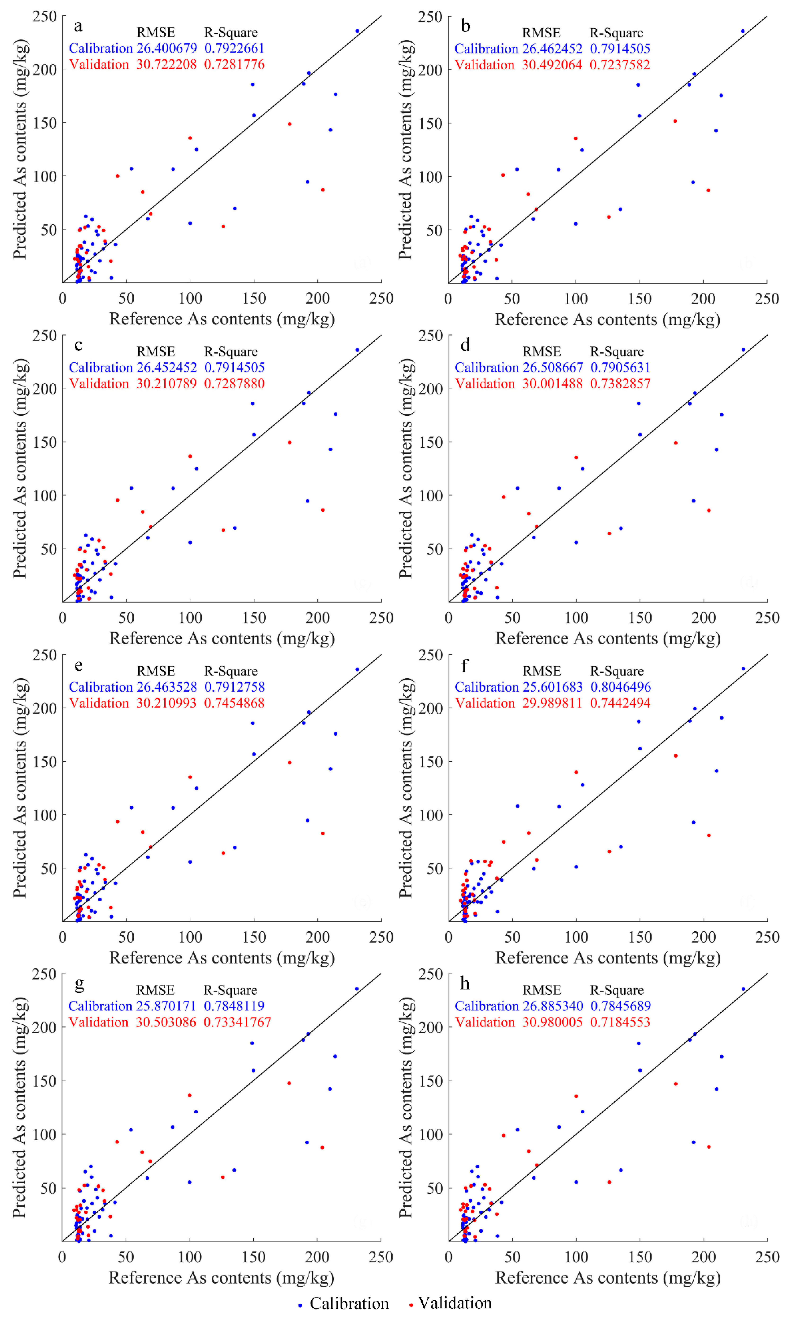
PLSR models using soil samples with 2 nm, 4 nm, 6 nm, 8 nm, 10 nm, 12 nm, and 14 nm spectral interval resampling were built for AS content estimation. Scatter points of different resampling interval model results are showed in Figure 3. The closer the scatter points are to the 1:1 line, the higher the accuracy and stability of the models are. Table 3 compares the modeling accuracy of different interval resampling spectrum using PLSR models. Different resampling intervals cause different accuracy; 10 nm interval resampling has the highest calibration and validation accuracy, indicating that spectral resampling at intervals of 10 nm can reduce spectral noise, remove redundant information, and maintain spectral data characteristics better. The bands referred to in the following sections, such as 690 nm, represent the arithmetic mean of 690–699 nm, 700 nm represents the arithmetic mean of 700–709 nm, and so on.

3.3. Different Spectral Preprocessing Method Modeling Results

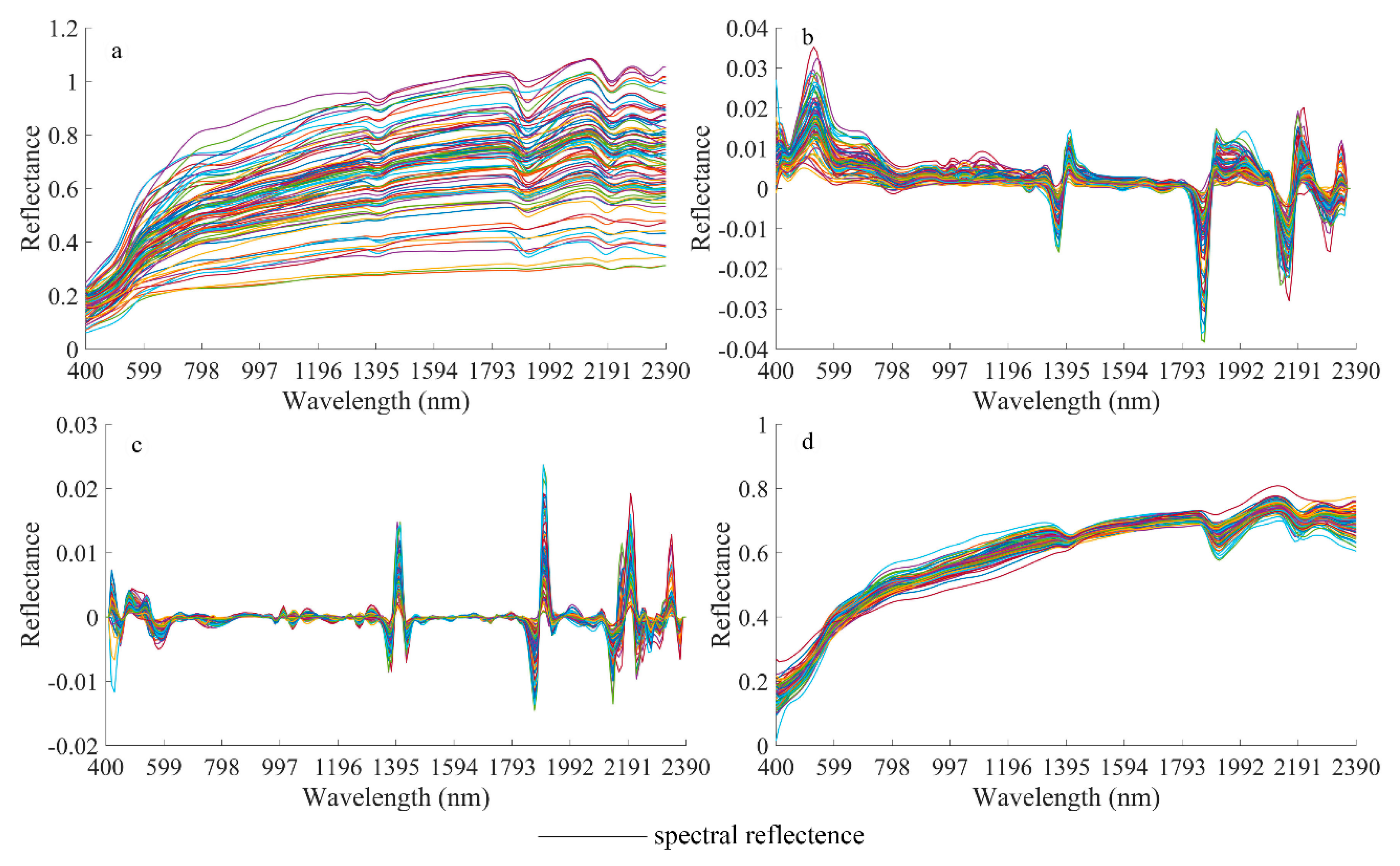
The curves of different spectral preprocessing methods are displayed in Figure 4. PLSR modeling was performed using four spectral data with different spectral pretreatments. The results of the different spectral preprocessing models are shown in Figure 5, which indicates that the position relationships between the scatter points and the 1:1 line are similar. However, the scatter point distribution of the SD model is closer to the 1:1 line. Table 4 shows the accuracy evaluation results of PLSR modeling after different preprocessing methods. It can be seen that the modeling accuracy of the four groups after different preprocessing methods is higher than that without the spectral preprocessing. After SD transformation, the modeling accuracy was the best, followed by SG, and MSC was the worst.

3.4. Influence of Feature Band Extraction on Segment Modeling Accuracy

Principal component analysis was performed on the 10 nm resampled and SD-transformed spectral data. Table 5 shows that the cumulative explained variance of the first six principal components has reached 95%. Therefore, the 55 original bands with the largest absolute value of correlation loadings from the first six principal components can be selected as the characteristic bands (Table 6). The reflectance of 55 feature bands is the independent variable, and the AS content is the dependent variable. Figure 6 shows the modeling result of the PLSR method. The comparison between the characteristic band and the full band modeling accuracy is displayed in Table 7. It can be seen that, compared with the PLSR modeling results of the feature band extraction by principal component analysis, the RMSE of the full-band modeling is lower, and R2 and RPD are higher, indicating that feature bands cannot improve the model verification accuracy in this study.

3.5. Different Inversion Model Modeling Results

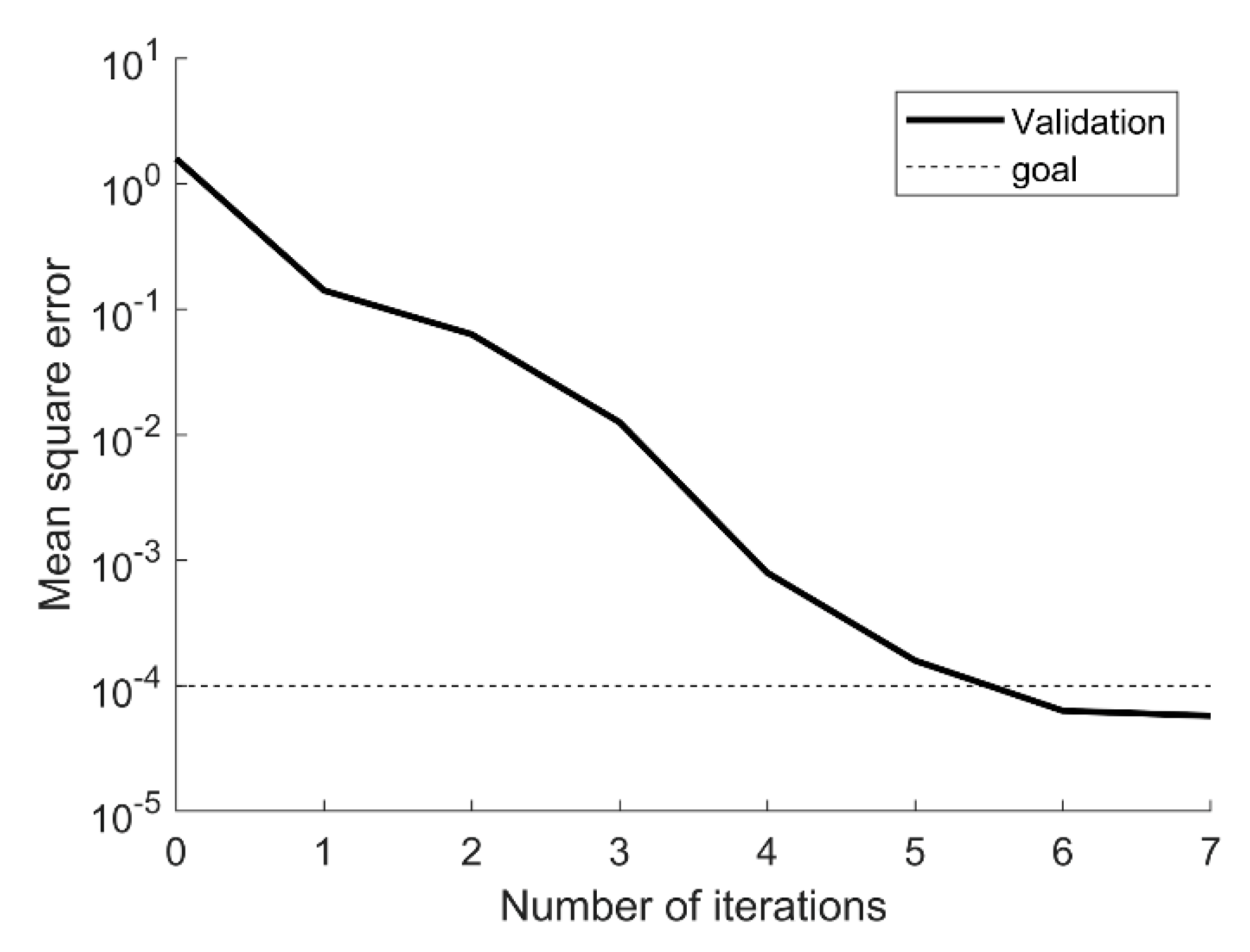
The spectral reflectance with 10 nm resampling and SD transformation is independent, and the AS content is used as the dependent variable. The model is established by PLSR, SVR, and BPNN, respectively. In the back propagation neural network model, the number of input layers, hidden layers, and output layers of the BP neural network model was 1. The number of neurons in the input layer was 200, the number of hidden layer neurons was 7, and the number of output layers was 1. The initial learning rate, η , was 0.11, the training frequency was 20, and the expected error was 0.0001. The error performance curve of BP neural network training is shown in Figure 7. After only six iterations, the network reached the expected error level, showing the fast convergence speed of the model. Figure 8 shows the modeling results. Most of the scatter points in BPNN are located close to the 1:1 line, and the trend is more consist with the 1:1 line. Table 8 compares the modeling accuracy of different modeling methods under the same interval spectral resampling and pretreatment conditions. In the BPNN modeling results, the difference of R2 between the calibration set and the validation set was 0.0715 and the difference in accuracy was only 7.67%, which indicates that the established BPNN model has good applicability and there is not an over-fitting problem in the model. After analyzing and comparing the results of the three models, it can be seen that the BPNN model was the best model for predicting the AS content in soil. This means that the BPNN model can solve the problem of the number of training samples being insufficient to support modeling due to excessive differences between sample values. The superiority of the BPNN model was attributed to the optimization of the BPNN initial input parameters (thresholds and weights); this approach does not have the problem of low accuracy common in other models.

4. Discussion

4.1. Best Inversion Model Analysis

In this paper, PLSR, SVR, and BPNN methods are used to establish a hyperspectral prediction model for estimating soil AS content in mining and suburban soils form VNIR spectra. Some studies regarding the models for estimating AS concentrations from VNIR spectrum are displayed in Table 9. By comparing the R2 and RPD values, our estimation using the BPNN model for AS is better than most of them, and the validation set, R2, and RPD are 0.861 and 2.536, respectively.
From Figure 3, Figure 5, Figure 6 and Figure 8a, it can be seen that the scatter points of the high soil AS content in the PLSR and SVR models are farer from the 1:1 line than in the BPNN model. This is because the number of the high soil AS content samples used for modeling are low and the extreme values between the sample values are too large. In the BPNN modeling results (Figure 8b), the scatter points of high soil AS content are relatively close to the 1:1 line, but there are still some points that are a long way from the line of equivalence. This maybe because the amount of data is too small and the model needs further optimization. Moreover, there are many factors affecting soil spectral, which may affect the modeling result. In general, BPNN has some strong abilities of adaptive learning, knowledge reasoning, and computational optimization. Therefore, the BPNN model can solve the nonlinear problem effectively between soil AS content and reflectance spectra, and the low modeling accuracy caused by insufficient data in other models can be avoided in order to improve model accuracy and stability simultaneously.

4.2. Inversion Mechanism Analysis

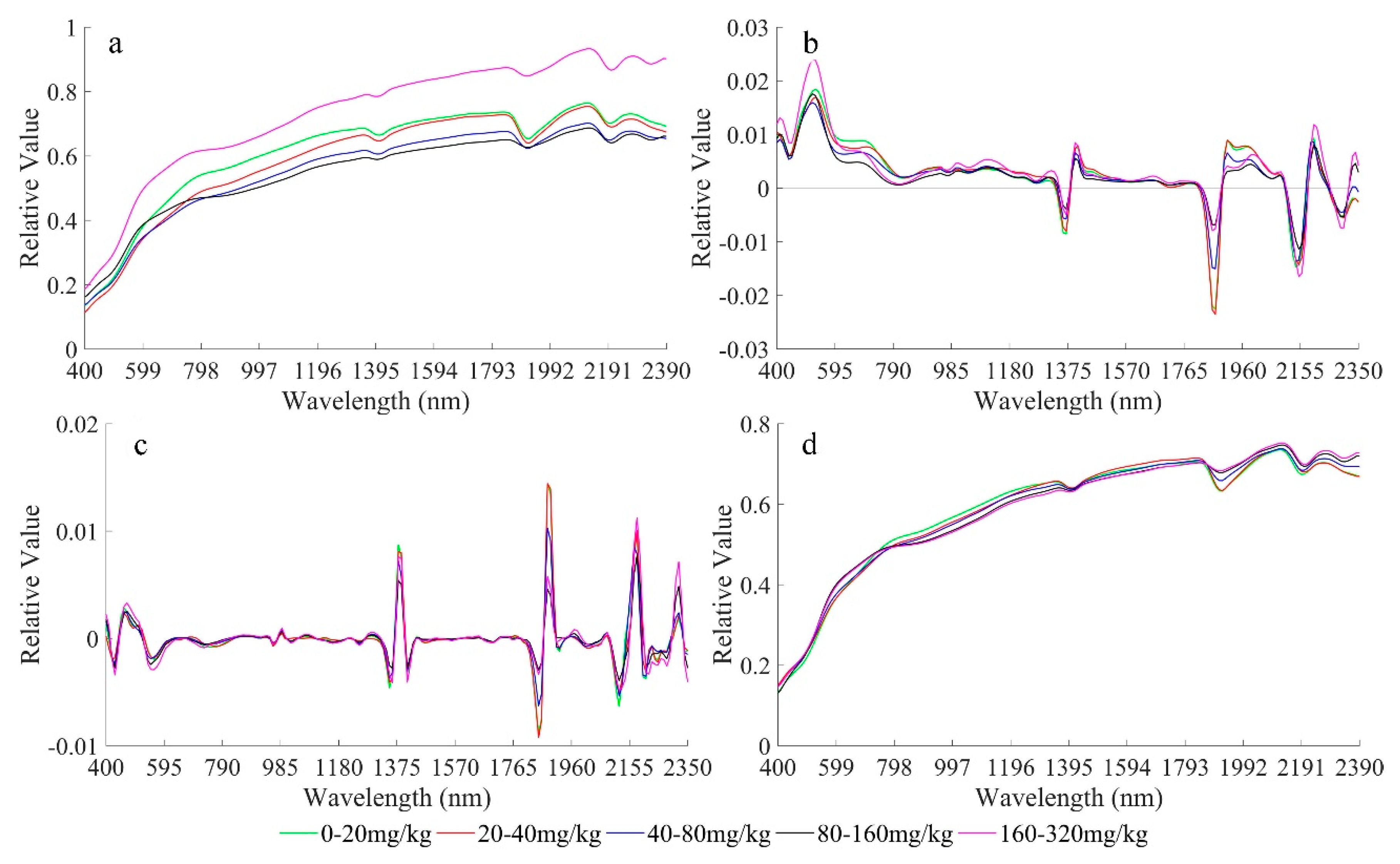
Many previous studies have shown that there are several weak absorption peaks at 430, 530, and 650 nm in the original spectrum, which are mainly related to iron-manganese oxide [35]. The absorption peaks at 1400, 1900, and 2210 nm are related to soil organic matter, clay minerals, and hydroxyl groups in the water [36]. The weak absorption peak at 2250 nm is mainly related to soil organic matter [37]. The 10 nm interval spectral resampling data subjected to different pretreatment methods were divided into five groups according to the AS content (Figure 9). The results show that SD transformation can effectively amplify the differences between spectral reflectance of feature bands with different AS contents, compared with S–G smoothing, FD, and MSC. This is the reason why SD transformation can improve the accuracy and stability of the model. There are some different degrees of reflection (absorption) peaks at 430, 530, 1380, 1400, 1430, 1870, 1900, 2140, 2200, and 2340 nm, which can be considered as characteristic bands of soil AS content, consistent with the characteristic bands of Fe (450, 550, 1000, 1400, 1900, 2050, 2200, 2250, 2400, and 2470 nm) [38]. Moreover, studies have shown that soil AS content is highly correlated with soil Fe content [35]. These indicate that the inversion mechanism of soil AS content is indirectly constructed by the correlation between AS and iron-manganese oxide, organic matter, and clay minerals.
In addition, some results suggest that the reflectance at 480, 1755, 1920, 2210, 2260, and 2320 nm have a good correlation with soil AS content [39]. The feature bands of soil AS content extracted by principal component regression were 450, 500, 600, 650, 700, 750, 800, 900, 1000, 1200, 1400, 1900, 2050, 2200, 2250, 2350, 2400, and 2470 nm [14]. These are consistent with this paper, indicating that the extraction results of feature bands are reliable. The modeling accuracy of the feature bands in Section 3.3 is slightly lower than the full-band modeling accuracy. This may be because the 10 nm interval spectral resampling has effectively eliminated the inter-spectral redundancy and repeated information, and the feature band extraction causes the effective information to be missing.

4.3. Limitations and Future Work

The presence of AS in soils is an issue of concern. Relative to the total AS content, the existing forms of AS is of great significance for understanding the source, migration, transformation characteristics, and bioavailability of AS in the soil. At present, most research on soil AS existence focusses on the areas of bio-remediation and phytoremediation [40]. According to the National Standard Soil environmental quality Risk control standard for soil contamination of agricultural land [33] and Soil environmental quality Risk control standard for soil contamination of development land [34] of the People’s Republic of China, the determination method of AS in soil is total AS element content. In order to compare with national standards, the total AS content in this study was used as the research object. Obviously, the estimation of AS content in different existing forms is a question worthy of discussion. However, the differences in the spectral characteristics of different AS content are not significant, and the detection method is difficult. In published research that estimate soil AS content based on hyperspectral, there is little research in estimating the AS content in different existing forms based on hyperspectral, but it is of great importance to distinguish the spectral differences in the AS content of different existing forms. We are also actively exploring this work.
The extreme value of soil AS suitable for hyperspectral estimation is still unknown, which is also a question worth exploring. In order to increase the range of AS content in soil samples, when selecting the study area, we selected a mining area with very high AS content and an urban suburb with low AS content. The 90 samples were divided into five groups: 0–20mg/kg, 20–40 mg/kg, 40–80 mg/kg, 0–160 mg/kg, and 160–320 mg/kg, and the accuracy and stability of the BPNN model were, respectively, calculated. The results are shown in Table 10. From the current sample data and test results, there is not much relationship between different AS content ranges and estimation accuracy, but it seems that the accuracy is higher when the amount of data is larger. Therefore, the study may be limited to individual sample points. In order to improve the estimation accuracy of soil AS content, it is necessary to collect more soil samples with high AS content in the future to optimize the soil AS content estimation models.
Hyperspectral estimation of soil AS content is fast and cost saving and provides some convenience for monitoring soil AS pollution. However, soil spectral reflectance is affected by multiple components [41,42]; in order to obtain accurate spectral information, soil samples need to be carefully measured. Therefore, in areas with large differences in soil composition, the application of this model needs to be discussed. As the number of soil samples increases, we will continue to optimize the models.

5. Conclusions

In this paper, we explored the feasibility and best estimation method for estimating soil AS content by BPNN and VNIR hyperspectral. The main conclusions are as follows: (1) The results of the PLSR models modeling using the original spectrum, 2, 4, 6, 8, 10, 12, and 14 nm interval resampling spectrum indicated that the estimation accuracy of 10 nm interval resampling is the best ( R v 2 = 0.744 and RPD = 1.725). (2) S–G smoothing was performed on the spectral data after 10 nm interval resampling, then FD, SD, and MSC transformation were performed, and the estimation model was established by the PLSR method. The results indicated that the SD transformation had the best modeling accuracy ( R v 2 = 0.770 and RPD = 1.887). (3) Comparing the PLSR modeling accuracy with the full-bands and 55 feature bands extracted by principal component analysis, the results suggested that the feature band extraction cannot improve the model validation accuracy. (4) The independent variable was the original spectral reflectance after 10 nm re-sampling and SD transform, and the dependent variable was AS content. The estimation models were established using PLSR, SVR, and BPNN algorithms, respectively. The results showed that BPNN had the best modeling accuracy ( R v 2 = 0.861 and RPD = 2.536). In summary, using BPNN and hyperspectral data to estimate soil AS content is feasible, and the best estimation method is: 10 nm+ SD+ BPNN.

Author Contributions

research conceptualization, L.H.; methodology, L.H., H.Z., and Y.Z.; investigation, L.H., R.C., Z.L., and H.H.; resources, H.Z.; writing, R.C. and L.H. All authors have read and agreed to the published version of the manuscript.

Funding

This study was funded by the Opening fund of the Key Laboratory of Degraded and Unused Land Consolidation Engineering, the Ministry of Land and Resources (Program No. SXDJ2017-9), the Opening fund of Shaanxi Key Laboratory of Land consolidation (Program No. 2018-ZZ03, 2018-JC03), the National Natural Science Foundation of China (Program No. 41871190), and the National Science Basic Research Plan in Shaanxi Province of China (Program No. 2018JQ4027). The sponsors had no role in the design, execution, interpretation, or writing of the study.

Conflicts of Interest

The authors declare no conflict of interest.

References

  1. Herath, I.; Vithanage, M.; Bundschuh, J.; Maity, J.P.; Bhattacharya, P. Natural Arsenic in Global Groundwaters: Distribution and Geochemical Triggers for Mobilization. Curr. Pollut. Rep. 2016, 2, 68–89. [Google Scholar] [CrossRef] [Green Version]
  2. Holly, M. An arsenic forecast for China. Science 2013, 341, 852–853. [Google Scholar]
  3. Iva, H. Arsenic in rice: A cause for concern. J. Pediatr. Gastroenterol. Nutr. 2015, 60, 142–154. [Google Scholar]
  4. Chao, S.; Jiang, J.Q.; Zhang, W.J. A review on heavy metal contamination in the soil worldwide: Situation, impact and remediation techniques. Environ. Skept. Crit. 2014, 3, 24–38. [Google Scholar]
  5. Guha, M.D.N.; Debasree, D.; Anirban, B.; Chandan, S.; Ashoke, N.; Arabinda, D.; Aloke, G.; Kallol, B.; Kanti, M.K. Dietary arsenic exposure with low level of arsenic in drinking water and biomarker: A study in West Bengal. J. Environ. Sci. Health Part A-Toxic/Hazard. Subst. Environ. Eng. 2014, 49, 555–564. [Google Scholar]
  6. Sobhanardakani, S. Arsenic health risk assessment through groundwater drinking (case study: Qaleeh shahin agricultural region, kermanshah province, Iran). Pollution 2009, 4, 77–82. [Google Scholar]
  7. Gong, H.M.; Ma, R.J.; Wang, Z.J.; Ye, Y.; Hu, Y.M. Development of Technologies for Monitoring Agricultural Soil Heavy Metal Pollution. Chin. Agric. Sci. Bull. 2013, 29, 140–147. [Google Scholar]
  8. Zhu, X.C.; Cao, L.G.; Liang, Y. Spatial distribution and risk assessment of heavy metals inside and outside a typical lead-zinc mine in southeastern China. Environ. Sci. Pollut. Res. 2019, 26, 26265–26275. [Google Scholar] [CrossRef]
  9. Sørensen, L.K.; Dalsgaard, S. Determination of Clay and Other Soil Properties by Near Infrared Spectroscopy. Soil Sci. Soc. Am. J. 2005, 69, 159. [Google Scholar] [CrossRef]
  10. Zhang, Q.X.; Zhang, H.B.; Liu, W.K.; Zhao, S.X. Inversion of heavy metals content with hyperspectral reflectance in soil of well-facilitied capital farmland construction areas. Trans. Chin. Soc. Agric. Eng. 2017, 33, 230–239. [Google Scholar]
  11. Yu, X.; Liu, Q.; Wang, Y.B.; Liu, X.Y.; Liu, X. Evaluation of MLSR and PLSR for estimating soil element contents using visible/near-infrared spectroscopy in apple orchards on the Jiaodong peninsula. Catena 2016, 137, 340–349. [Google Scholar] [CrossRef]
  12. Zheng, G.H.; Zhou, S.L.; Wu, S.H. Prediction of As in Soil with Reflectance Spectroscopy. Environ. Sci. Pollut. Res. 2011, 31, 173–176. [Google Scholar]
  13. Cheng, H.; Shen, R.L.; Chen, Y.Y.; Wan, Q.J.; Shi, T.Z.; Wang, J.J.; Wan, Y.; Hong, Y.S.; Li, X.C. Estimating heavy metal concentrations in suburban soils with reflectance spectroscopy. Geoderma 2019, 336, 59–67. [Google Scholar] [CrossRef]
  14. Ren, H.Y.; Zhuang, D.F.; Qiu, D.S.; Pan, J.Q. Analysis of Visible and Near-Infrared Spectra of As Contaminated Soil in Croplands Beside Mines. Spectrosc. Spectr. Anal. 2009, 29, 114–118. [Google Scholar]
  15. Wu, Y.Z.; Chen, J.; Ji, J.F.; Gong, P.; Liao, Q.L.; Tian, Q.J.; Ma, H.R. A Mechanism Study of Reflectance Spectroscopy for Investigating Heavy Metals in Soils. Soil Sci. Soc. Am. J. 2007, 71, 918–926. [Google Scholar] [CrossRef]
  16. Wu, D.W.; Wu, J.Z.; Ma, H.R. Study on the Prediction of Soil Heavy Metal Elements Content Based on Mid-Infrared Diffuse Reflectance Spectra. Spectrosc. Spectr. Anal. 2010, 30, 1498–1502. [Google Scholar]
  17. Zhang, W.; Gao, X.H.; Yang, Y.; Li, J.S.; Zhang, Y.J.; Tian, C.M.; Jia, W.; Feng, L.; Ma, Y.L.; Yuan, H.X.; et al. Estimating Heavy Metal Contents for Topsoil Based on Spectral Analysis —A Case Study of Yushu and Maduo Counties in the Three-River Source Region. Soils 2014, 46, 1052–1060. [Google Scholar]
  18. Wang, J.J.; Cui, L.J.; Gao, W.X.; Shi, T.Z.; Chen, Y.Y.; Gao, Y. Prediction of low heavy metal concentrations in agricultural soils using visible and near-infrared reflectance spectroscopy. Geoderma 2014, 216, 1–9. [Google Scholar] [CrossRef]
  19. Liu, P.; Liu, Z.H.; Hu, Y.M.; Shi, Z.; Pan, Y.C.; Wang, L.; Wang, G.X. Integrating a Hybrid Back Propagation Neural Network and Particle Swarm Optimization for Estimating Soil Heavy Metal Contents Using Hyperspectral Data. Sustainability 2019, 11, 419. [Google Scholar] [CrossRef] [Green Version]
  20. Xu, L.J.; Li, Q.Q.; Zhu, X.M.; Liu, S.G. Hyperspectral Inversion of Heavy Metal Content in Coal Gangue Filling Reclamation Land. Spectrosc. Spectr. Anal. 2017, 37, 3839–3844. [Google Scholar]
  21. Tan, K.; Ye, Y.Y.; Du, P.J.; Zhang, Q.Q. Estimation of Heavy Metal Concentrations in Reclaimed Mining Soils Using Reflectance Spectroscopy. Spectrosc. Spectr. Anal. 2014, 34, 3317–3322. [Google Scholar]
  22. Mutanga, O.; Skidmore, A.K.; Prins, H.H.T. Predicting in situ pasture quality in the Kruger National Park, South Africa, using continuum-removed absorption features. Remote Sens. Environ. 2003, 89, 393–408. [Google Scholar] [CrossRef]
  23. Zhao, L.; Hu, Y.M.; Zhou, W.; Liu, Z.H.; Pan, Y.C.; Shi, Z.; Wang, L.; Wang, G.X. Estimation Methods for Soil Mercury Content Using Hyperspectral Remote Sensing. Sustainability 2018, 10, 2474. [Google Scholar] [CrossRef] [Green Version]
  24. Curran, P.J.; Dungan, J.L.; Peterson, D.L. Estimating the foliar biochemical concentration of leaves with reflectance spectrometry. Remote Sens. Environ. 2001, 76, 349–359. [Google Scholar] [CrossRef]
  25. Fukunaga, K.; Koontz, W.L.G. Representation of random processes using the finite Karhunen-Loève expansion. Inf. Control 1970, 16, 85–101. [Google Scholar] [CrossRef] [Green Version]
  26. Wang, H.W. Partial Least Squares Regression Method and its Application; National Defense Industry Press: Beijing, China, 1999; pp. 1–3. [Google Scholar]
  27. Hsu, C.; Lin, C. A comparison of methods for multiclass support vector machines. IEEE Trans. Neural Netw. 2008, 13, 415–425. [Google Scholar]
  28. Liu, X.B. Analysis and Research of Forecast Model on PM2.5 Using Support Vector Regression. Master’s Thesis, Southwestern University Of Finance And Economics, Chengdu, China, 2016. [Google Scholar]
  29. Lian, C.Y. Support Vector Regression Based on Genetic Algorithm and its Application in Phase Separation Procedure with Salts. Master’s Thesis, Hebei University Of Technology, Wuhan, China, 2015. [Google Scholar]
  30. Zhou, Z.H. Neural Network and its Application; Tsinghua University Press: Beijing, China, 2004. [Google Scholar]
  31. Esbensen, K.H.; Guyot, D.; Westad, F.; Lars, P.H. Multivariate Data Analysis: An Introduction to Multivariate Data Analysis and Experimental Design, 5th ed.; CAMO Software: Oslo, Norway, 2002; p. 598. [Google Scholar]
  32. Si, H.Q.; Yao, Y.M.; Qang, D.Y.; Liu, Y. Hyperspectral prediction of soil organic matter contents under different soil moisture contents. Trans. Chin. Soc. Agric. Eng. 2015, 31, 114–120. [Google Scholar]
  33. GB 15618-2018. Soil Environmental Quality—Risk Control Standard for Soil Contamination of Agricultural Land; Ministry of Ecology and Environment of the People’s Republic of China: Beijing, China, 2018. Available online: http://www.mee.gov.cn/ywgz/fgbz/bz/bzwb/trhj/201807/t20180703_446029.shtml. (accessed on 2 November 2019).
  34. GB 36600-2018. Soil Environmental Quality—Risk Control Standard for Soil Contamination of a Development Land; Ministry of Ecology and Environment of the People’s Republic of China: Beijing, China, 2018. Available online: http://www.mee.gov.cn/ywgz/fgbz/bz/bzwb/trhj/ (accessed on 3 November 2019).
  35. Wu, Y.Z.; Chen, J.; Wu, X.M.; Tian, Q.J.; Ji, J.F.; Qin, Z.H. Possibilities of reflectance spectroscopy for the assessment of contaminant elements in suburban soils. Appl. Geochem. 2005, 20, 0–1059. [Google Scholar] [CrossRef]
  36. Nayak, P.S.; Singh, B.K. Instrumental characterization of clay by XRF, XRD and FTIR. Bull. Mat. Sci. 2007, 30, 235–238. [Google Scholar] [CrossRef] [Green Version]
  37. Ben-Dor, E.; Inbar, Y.; Chen, Y. The reflectance spectra of organic matter in the visible near-infrared and short wave infrared region (400–2500 nm) during a controlled decomposition process. Remote Sens. Environ. 1997, 61, 1–15. [Google Scholar] [CrossRef]
  38. Thomas, K.; Stefan, S. Estimate of heavy metal contamination in soils after a mining accident using reflectance spectroscopy. Environ. Sci. Technol. 2002, 36, 2742–2747. [Google Scholar]
  39. Song, l.; Jian, J.; Tan, D.J.; Xie, H.B.; Luo, Z.F.; Gao, B. Estimation of soil’s heavy metal concentration (As, Cd and Zn) in Wansheng mining area with geochemistry and field spectroscopy. Spectrosc. Spectr. Anal. 2014, 34, 812–817. [Google Scholar]
  40. Zhao, F.J.; McGrath, S.P.; Meharg, A.A. Arsenic as a food chain contaminant: Mechanisms of plant uptake and metabolism and mitigation strategies. Annu. Rev. Plant Biol. 2010, 61, 535–559. [Google Scholar] [CrossRef] [PubMed] [Green Version]
  41. Gao, P.; Fu, T.G.; Wang, K.L.; Chen, H.Y.; Zeng, F.P. Spatial heterogeneity of surface soil mineral components in a small catchment in Karst peakcluster depression area, South China. Chin. J. Appl. Ecol. 2013, 24, 3179–3184. [Google Scholar]
  42. Liu, H.J.; Wang, X.; Li, H.X.; Meng, X.T.; Jiang, B.W.; Zhang, X.L.; Yu, Z.Y. Effect mechanism of soil minerals on spectral characteristics of main soil classes in songnen plain. Spectrosc. Spectr. Anal. 2018, 38, 3238–3244. [Google Scholar]
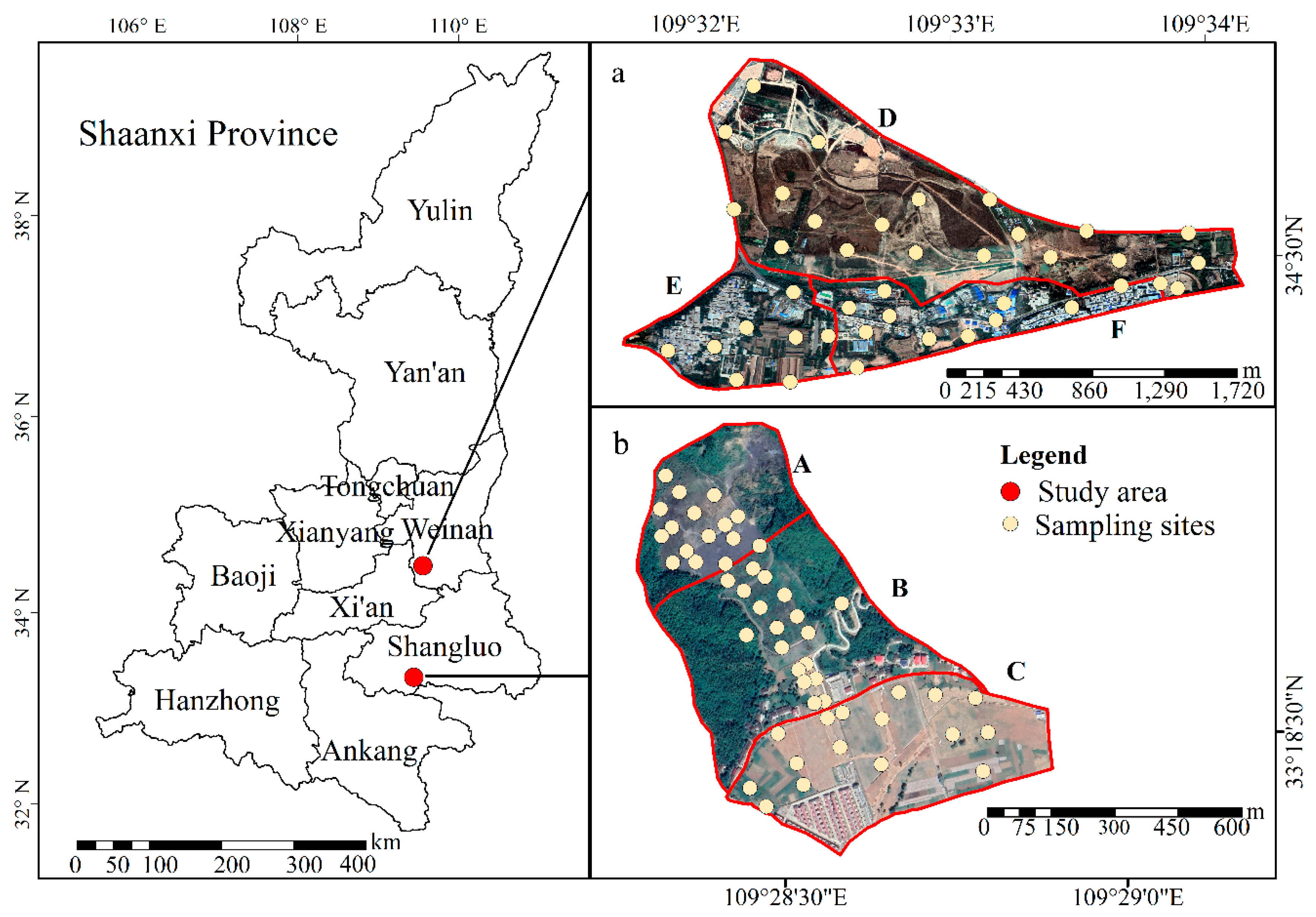
Figure 1. Study area and the distribution of soil sampling points; A–F denote six types of land use, (a) suburb, Weinan City, (b) mining area, Shangluo City.
Sustainability 12 01476 g001
Figure 2. Back Propagation neural network (BPNN) topology structure.
Sustainability 12 01476 g002
Figure 3. Scatter plots of the reference vs predicted arsenic contents for different resample intervals using partial least squares regression: (a) original, (b) 2 nm, (c) 4 nm, (d) 6 nm, (e) 8 nm, (f) 10 nm, (g) 12 nm, and (h) 14 nm. RMSE: root mean square error.
Sustainability 12 01476 g003
Figure 4. The spectral reflectance curves of the soil samples; (a) Savitzky–Golay (S-G), (b) First Derivation (FD), (c) Second Derivation (SD), and (d) Multiplicative Scatter Correction (MSC). (Each curve indicates the spectral curve of one soil sample).
Sustainability 12 01476 g004
Figure 5. Scatter plots of the reference vs. predicted soil arsenic contents for different spectral pretreatments using partial least squares regression; (a) S-G, (b) FD, (c) SD, and (d) MSC. The blue points indicate the calibration set and the red points indicates the validation set.
Sustainability 12 01476 g005
Figure 6. Scatter plots of the reference vs. predicted soil arsenic contents after selection feature bands using partial least squares regression.
Sustainability 12 01476 g006
Figure 7. Error of Back Propagation neural network.
Sustainability 12 01476 g007
Figure 8. Scatter plots of the reference vs. predicted soil arsenic contents using support vector regression (a) and back propagation neutral network (b) models.
Sustainability 12 01476 g008
Figure 9. Mean reflectance spectrum for five groups of resampling at 10 nm intervals and Savitzky–Golay (a), First Derivation (b), Second Derivation (c), and Multiplicative Scatter Correction (d) transformation, with AS content gradients.
Sustainability 12 01476 g009
Table 1. Soil arsenic (AS) concentrations and pH of soil samples in different areas.
Site TypeItemMaxMinMeanCoefficient of VariationBackground ValueRatio
Mining AreaAAS (mg/kg)231.0054.00150.700.37 **602.51
pH8.938.048.37
BAS (mg/kg)100.0013.3035.210.71 **251.41
pH8.565.338.19
CAS (mg/kg)41.5016.1025.880.28 **251.03
pH8.407.538.13
SuburbDAS (mg/kg)14.3011.3012.580.07600.21
pH9.138.408.81
EAS (mg/kg)16.1012.2013.550.08 **200.68
pH8.888.188.52
FAS (mg/kg)14.909.4012.530.12 *600.21
pH8.748.288.47
** means significant on 0.01 level, * means significant on 0.05 level. Take group D data as a control group.
Table 2. AS concentrations of soil samples in different data sets.
Data SetMax (mg/kg)Min (mg/kg)Mean (mg/kg)Coefficient of Variation
Calibration Set231.009.4045.611.28 **
Validation Set 214.0011.0045.011.27 **
** means significant on 0.01 level.
Table 3. The estimation results of different resample interval using partial least squares regression.
kRMSECRMSEV R C 2 R v 2 MAECMAEVRPD
Original526.4030.720.79230.728216.976322.63541.6546
2 nm426.5230.490.79150.723816.840622.22151.6655
4 nm326.4530.210.79150.728816.523621.65471.6989
6 nm326.5130.000.79060.738315.445921.36451.6922
8 nm326.4630.210.79130.745515.432122.21561.6592
10 nm325.6029.990.80460.744215.398120.54421.7253
12 nm326.3730.500.78480.733416.256421.19651.6543
14 nm326.8930.980.78460.718517.336522.03981.6312
k: the number of partial least squares regression (PLSR) factors used in each calibration. RMSEC: the root mean square error of the calibration set. RMSEV: the root mean square error of the validation set. R C 2 : the coefficient of determination of the calibration set. R V 2 : the coefficient of determination of the validation set. MAEC: the mean absolute error of the calibration set. MAEV: the mean absolute error of the validation set. RPD: residual predictive deviation.
Table 4. The estimation results of different spectral pretreatments using partial least squares regression.
kRMSECRMSEV R C 2 R v 2 MAECMAEVRPD
Original325.6029.990.80460.744315.398120.54421.7253
S–G325.6828.010.80340.766115.498821.35611.8576
FD426.0428.200.79800.757915.832220.54141.8375
SD424.9027.770.81520.770116.889914.62931.8874
MSC329.7132.240.73690.689219.930720.52291.5499
S–G: Savitzky–Golay. FD: first derivation. SD: second derivation. MSC: multiplicative scatter correction.
Table 5. The accumulated explained variance of the first 10 principal components (PC) of soil reflectance spectral.
Principal ComponentPC1PC2PC3PC4PC5PC6PC7PC8PC9PC10
Cumulative (%)53.672.885.892.594.195.696.697.397.898.2
Table 6. Feature band extraction results.
Soil PropertiesFeature Bands/nm
AS430, 450, 470, 480, 530, 610, 620, 640–660, 1030–1060, 1080–1110, 1230, 1240, 1280, 1300–1320, 1360–1380, 1400, 1400, 1480, 1510, 1580, 1750, 1850–1930, 2050, 2120, 2140, 2160, 2170, 2190–2220, 2250, 2340–2360
Table 7. The estimation results of the feature bands and all-bands using partial least squares regression.
kRMSECRMSEV R C 2 R v 2 MAECMAEVRPD
Feature Bands226.8629.620.78500.738422.108424.54371.7389
All-bands424.9027.770.81520.770114.629316.88991.8874
Table 8. The estimation results of using partial least squares regression, support vector regression, and a back propagation neutral network.
RMSECRMSEV R C 2 R v 2 MAECMAEVRPD
PLSR24.9027.770.81520.770114.629316.88991.8874
SVR32.8034.170.75700.720116.615920.31211.0313
BPNN16.5920.290.93220.860711.274914.42262.5362
Table 9. Comparison of the estimation models of AS concentration in soils using visible and reflectance spectroscopy.
Sampling SiteNum.MethodsR2RPDReferences
Agricultural Soils33MSC + PCR0.3674 [14]
Suburban Area61FD + PLSR0.72001.9000[15]
Suburban Area93SG + PLSR0.75001.8100[13]
Urban Area161SG + PLSR0.67001.7200[16]
Urban Area974nm + MSC + PLSR0.71101.8270[12]
Urban Area154BD + MLR0.39001.2300[17]
Urban Area96GA + PLSR0.35001.0900[18]
Urban Area90PSO + BPNN0.8110 [19]
Mining Area45SD + PLSR0.8400 [20]
Mining and Suburban Areas9010nm + SD + BPNN0.86072.5362This work
BD: band depth. GA: genetic algorithm. PSO: particle swarm optimization. RMSE: root mean square error. R 2 : coefficient of determination.
Table 10. The estimation results of different AS content ranges using back propagation neural networks.
AS ContentNumber of SampleRMSECRMSEV R C 2 R v 2 MAECMAEVRPD
0–20 mg/kg5213.3116.520.92540.873611.589613.63542.825
20–40 mg/kg1815.4918.860.91090.868911.861414.21452.757
40–80 mg/kg619.1821.900.98520.849612.201614.2492.365
80–160 mg/kg819.3423.630.87610.859912.025413.99652.412
160–320 mg/kg817.0921.360.88150.860612.632114.62542.613