Intelligence in Tourist Destinations Management: Improved Attention-based Gated Recurrent Unit Model for Accurate Tourist Flow Forecasting

Abstract

Accurate tourist flow forecasting is an important issue in tourist destinations management. Given the influence of various factors on varying degrees, tourist flow with strong nonlinear characteristics is difficult to forecast accurately. In this study, a deep learning method, namely, Gated Recurrent Unit (GRU) is used for the first time for tourist flow forecasting. GRU captures long-term dependencies efficiently. However, GRU’s ability to pay attention to the characteristics of sub-windows within different related factors is insufficient. Therefore, this study proposes an improved attention mechanism with a horizontal weighting method based on related factors importance. This improved attention mechanism is introduced to the encoding–decoding framework and combined with GRU. A competitive random search is also used to generate the optimal parameter combination at the attention layer. In addition, we validate the application of web search index and climate comfort in prediction. This study utilizes the tourist flow of the famous Huangshan Scenic Area in China as the research subject. Experimental results show that compared with other basic models, the proposed Improved Attention-based Gated Recurrent Unit (IA-GRU) model that includes web search index and climate comfort has better prediction abilities that can provide a more reliable basis for tourist destinations management.

1. Introduction

Since the 2000s, the tourism industry in China has significantly increased given the rapid development of the Chinese economy. According to statistics, the number of inbound and domestic tourists in China is increasing annually, and the tourism industry is developing rapidly [1]. Especially during the peak months, the surge in the number of tourists has brought a series of problems to tourist destinations management, including unreasonable allocation of resources in tourist attractions and congestion of tourists. Therefore, accurate tourist flow forecasting is essential for tourist destination management.

However, daily tourist flow presents a complicated nonlinear characteristic because of the effects of various factors in varying degrees. Its complicated nonlinearity makes it difficult for existing methods to deal with the issue in an exact manner. Although accurate tourist flow forecasting remains a difficult task, it has attracted attention in the literature. Developing a new forecasting technique is necessary to obtain a satisfactorily accurate level.

1.1. Traditional Methods in Tourist Flow Forecasting

In recent years, various studies on tourist flow forecasting have resulted in the development of numerous forecasting methods. The early methods of tourist flow forecasting mainly include econometric [2] and time-series models [3]. Econometric models mainly include autoregressive distribution lag model [4], error correction model [5], and vector autoregressive model [6]. Time series models mainly include autoregressive moving average model [7] and autoregressive integrated moving average model [8,9]. These methods usually employ historical data to forecast future tourist flow through a univariate or multivariate mathematical function, which depends mostly on linear assumptions. These traditional methods have a good effect on tourist flow forecasting with linear characteristics. However, the prediction effect of these models on complex nonlinear tourist flow forecasting is inaccurate. Consequently, scholars have started to utilize machine-learning methods to build nonlinear prediction models, such as support vector regression [10,11] and artificial neural networks [12,13]. The artificial neural network methods have been used widely in tourist flow forecasting. These methods emulate the processes of the human neurological system to process self-learning from the historical tourist flow patterns, especially for nonlinear and dynamic variations. Accurate predictions can be obtained through repeated training and learning to approximate the real model. However, limitations are still observed in such methods, especially in addressing the sequence dependence among input variables in time series prediction.

1.2. Improved Attention-based Gated Recurrent Unit Model in Tourist Flow Forecasting

Recurrent Neural Network (RNN) is the most common and effective tool for time series models, especially in addressing sequence dependencies among input variables [14]. In the calculation of RNN, results are interdependent and the current input of the hidden layer is highly correlated with the last output. However, as the time series progresses, the problem of gradient disappearance becomes evident. To solve such a problem, a long short-time memory neural network (LSTM) [15] and Gated Recurrent Unit (GRU) [16] are proposed based on the original RNN. GRU is an improved model of LSTM, which controls the switch of memorizing and forgetting by setting multiple threshold gates. LSTM and GRU solve the limitation problem of handling long-term dependencies well. These methods have led to their successful application on various sequence learning problems, such as machine translation [17], speech recognition [18], and load forecasting [19,20]. LSTM has also been applied successfully for the first time in tourist flow forecasting [21]. In the study, LSTM was able to fit the test datasets and was proved to be superior to autoregressive integrated moving average model and backpropagation neural network, achieving the best performance in all cases. Therefore, LSTM and GRU are the most advanced methods for addressing time series prediction problems. LSTM and GRU can help capture long-term dependencies.

However, their ability to process information is still insufficient. Learning from cognitive neuroscience, researchers introduce attention mechanisms to the encoding–decoding framework [22,23] to select further from the input series and encode the information in long-term memory to improve information processing ability. In recent years, related works [24,25,26] on time series prediction are improved usually by introducing attention layers into the encoding-decoding framework. The attention mechanism has also been combined successfully with LSTM and applied to power forecasting [27], load forecasting [28], and travel time forecasting [29]. However, few articles in tourist flow forecasting have referred to this combined method. A cause of widespread concern is the work of Li et al. [30], wherein the attention mechanism was combined with LSTM and competitive random search (CRS) was used to configure the parameters of the attention layer, which improved the attention of LSTM to varying degrees of sub-window features in multiple time steps. However, although the attention mechanism improves the feature attention of LSTM in the time step, it remains insufficient for LSTM to pay different attention to sub-window features within different related factors. To solve such a problem, this study changes the vertical weighting method based on time importance and proposes an improved attention mechanism, which has horizontal weighting method based on factor importance. This improved attention mechanism is trained with CRS and then combined with GRU to increase the degree of attention of GRU to various related factors.

1.3. Web Search Index and Climate Comfort in Tourist Flow Forecasting

In the study of tourist flow forecasting, the prediction accuracy of the model is affected by the model itself and various factors. Moreover, existing studies have not considered other factors, such as web search index and climate comfort. Given the rapid development of the internet, people can easily search for information through search engines. At present, scholars believe that web search is an important and advanced way to obtain timely data and useful information [31]. When using the internet to search for data, the search history reflects the content of interest and the behavior that follows. In recent years, web search data has provided a new source of data and analytical basis for scientific research, which have been verified by researchers. For example, Choi and Varian have found in their research on Hong Kong’s tourist flow forecasting that the autoregressive model including Google search trends can improve prediction accuracy by at least 5% [32]. Prosper and Ryan have found that Google search trends can significantly improve forecasting results in the tourist flow forecasting studies on five tourist destinations in the Caribbean [33]. Similarly, Önder and Gunter have found in the study of tourist flow forecasting in major European cities that the Google search index can effectively improve the forecasting effect [34]. In view of various meteorological factors affecting tourist flow, climate comfort has gradually become a hot spot and the focus of tourism-related research. Li et al. have found in the tourism research on Hong Kong and other 13 major cities in China that climate comfort has a significant positive impact on the tourist flow in the mainland [35]. Chen et al. have included climate comfort in the model of Huangshan’s tourist flow forecasting and obtained better prediction results, indicating that climate comfort is significantly correlated with daily tourist flow [36]. Therefore, in this study, the web search index and climate comfort are used as important factors in tourist flow forecasting.

This study aims to propose a tourist flow forecasting method based on web search index, climate comfort, and Improved Attention-based GRU (IA-GRU) model. The CRS and attention mechanism are used to optimize the attention layer. Then, the selected web search index and climate comfort are added to improve the forecasting effect of IA-GRU model. The results of this study demonstrate the effectiveness of this model. The remaining parts of this paper are organized as follows. Section 2 introduces the basic principles of LSTM, GRU, attention mechanism, and IA-GRU model. Section 3 presents the data-processing methods using Huangshan Scenic Area as the research subject. Section 4 discusses the prediction performance of the proposed model and the comparison with other basic models. Section 5 provides the conclusion.

2. Methods

In this section, we discuss the structure of LSTM and GRU and explain why GRU is chosen as the prediction model. Then, we provide the outline for the attention mechanism and the details of the IA-GRU model. In addition, we train the IA-GRU model with a collaborative mechanism, which combines the attention mechanisms with CRS.

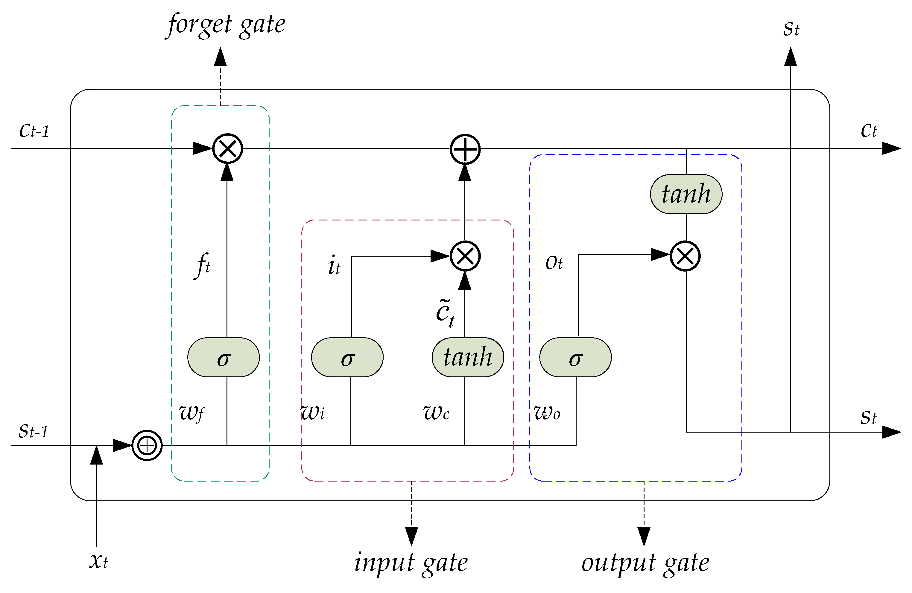
2.1. LSTM (GRU’s Precursor)

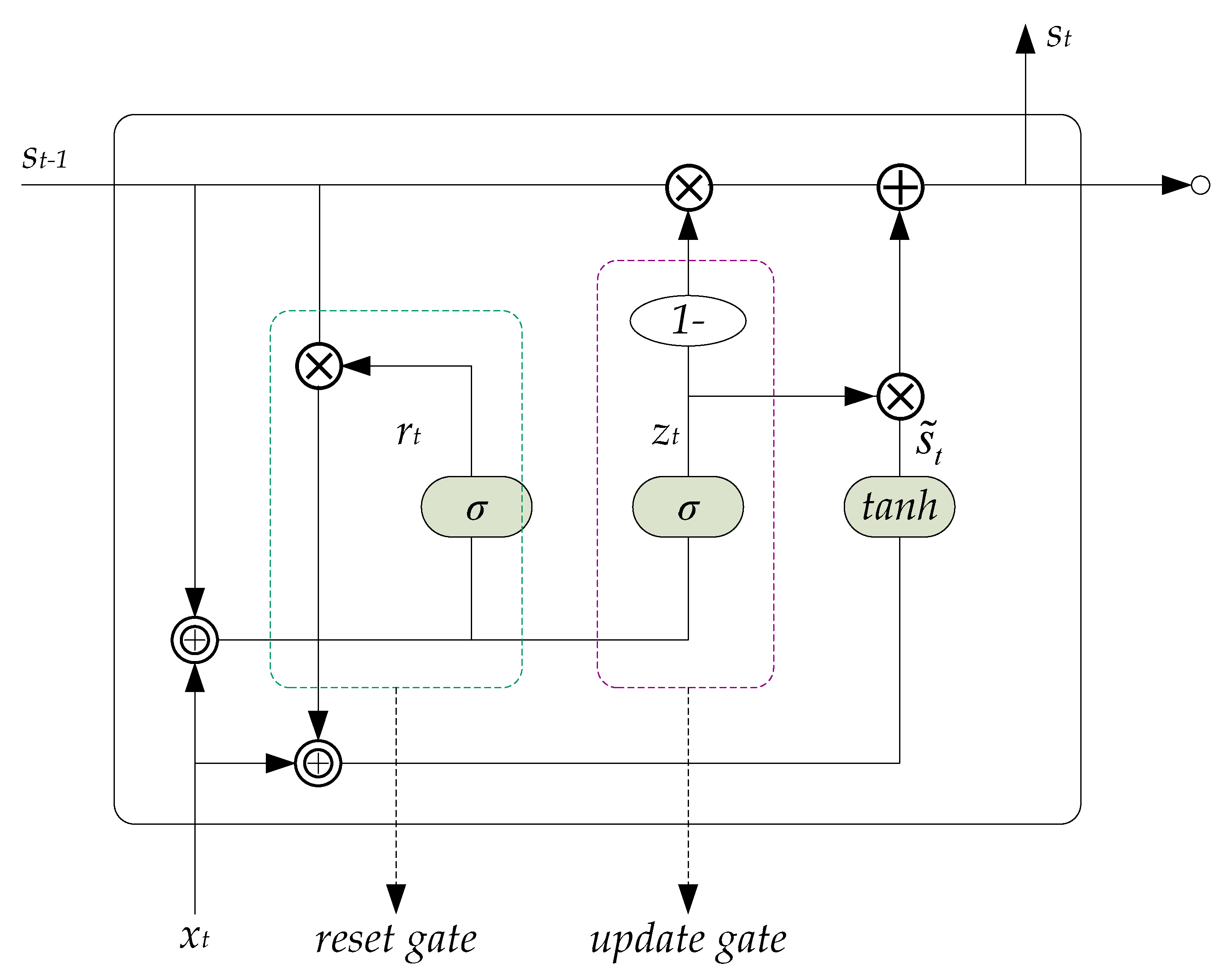
LSTM is first proposed for language models in 1997 [15]. LSTM is an RNN with a special structure, which has the advantage of being able to deal with the long-term dependency of time series. LSTM can solve the problem of gradient disappearance caused by RNN after multi-level network propagation.

As shown in Figure 1, one $tanh$ layer σ and three layers exist inside LSTM. The three layers correspond to three gates, namely, the forget gate, input gate, and output gate. The role of the horizontal line is to pass $c_{t-1}$ to $c_t$. The three gates and horizontal lines work together to complete the filtering and transmission processes of input information.

We denote the input time series as $x_t$, hidden state cells as $s_t$, and output sequence as $\widehat{y}$. LSTM neural networks perform the computation as follows:

$$f_t=\sigma (w_f\cdot [s_{t-1},x_t]+b_f),$$

(1)

$$i_t=\sigma (w_i\cdot [s_{t-1},x_t]+b_i),$$

(2)

$${\tilde{c}}_t=tanh(w_c\cdot [s_{t-1},x_t]+b_c),$$

(3)

$$c_t=f_t\ast c_{t-1}+i_t\ast {\tilde{c}}_t,$$

(4)

$$o_t=\sigma (w_o\cdot [s_{t-1},x_t]+b_o),$$

(5)

$$s_t=o_t\ast tanh(c_t),$$

(6)

$$\widehat{y}=w_y\cdot s_t+b_y,$$

(7)

where $\sigma$ and $tanh$ are activation functions applied to the internal structure of LSTM. Equations (8) and (9) are their calculation processes, respectively, wherein $\sigma$ stands for the standard sigmoid function. The output value of the $\sigma$ layer is between 0 and 1. The output value determines whether the input information can pass through the gate. A value of zero signifies “let nothing through,” whereas a value of one means “let everything through!” $f$, $i$, $o$, and $c$ respectively denote the mentioned inner-cell gates, namely, the forget gate, input gate, output gate, and cell activation vectors, $c$ should be equal to the hidden vector $s$. The $w$ terms denote weight matrices, whereas the $b$ terms denote bias terms. The input gate can determine how incoming vectors $x_t$ alter the state of the memory cell. The output gate can allow the memory cell to have an effect on the outputs. Then, the forget gate allows the cell to remember or forget its previous state.

$$\sigma (x)=\frac{1}{1+e^{-x}},$$

(8)

$$tanh(x)=\frac{e^x-e^{-x}}{e^x+e^{-x}}.$$

(9)

2.2. GRU

Given the complex structure of LSTM, the training of LSTM RNN often takes a lot of time. To improve the training speed and capture long-term dependencies efficiently, GRU is proposed as an improved model of LSTM in 2014 due to its simple structure and easy training [16]. The structure of the GRU is shown in Figure 2. Unlike LSTM, GRU has only two gates, namely, reset gate $r$ and update gate $z$.

We denote the input time series as $x_t$, hidden state cells as $s_t$, and output sequence as $\widehat{y}$. GRU neural networks perform the computation as follows:

$$r_t=\sigma (w_r\cdot [s_{t-1},x_t]),$$

(10)

$$z_t=\sigma (w_z\cdot [s_{t-1},x_t]),$$

(11)

$${\tilde{s}}_t=tanh(w\cdot [r_t\ast s_{t-1},x_t]),$$

(12)

$$s_t=(1-z_t)\ast s_{t-1}+z_t\ast {\tilde{s}}_t,$$

(13)

$$\widehat{y}=w_y\cdot s_t.$$

(14)

The reset gate $r$ determines the proportion of the output state $s_{t-1}$ at the previous moment in the new hidden state ${\tilde{s}}_t$. The new hidden state ${\tilde{s}}_t$ is obtained by performing a nonlinear transformation of the $tanh$ activation function on the output state at the previous moment $s_{t-1}$ and the input at the current moment $x_t$. The update gate $z$ mainly affects the proportion of the current hidden state $s_t$ in the new hidden state ${\tilde{s}}_t$. Concurrently, the update gate $z$ controls the proportion of ${\tilde{s}}_t$ and $s_{t-1}$ in the final output state $s_t$.

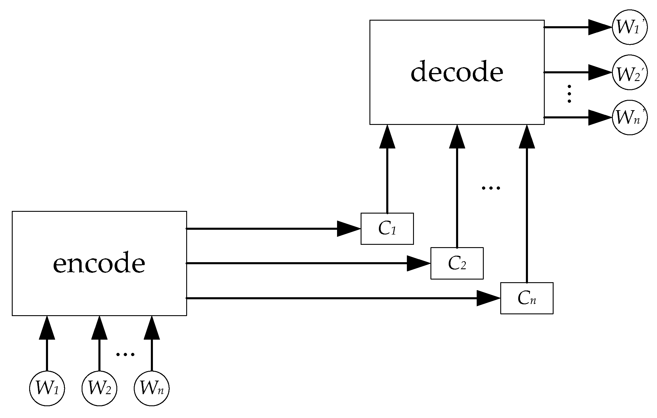
2.3. Attention Mechanism

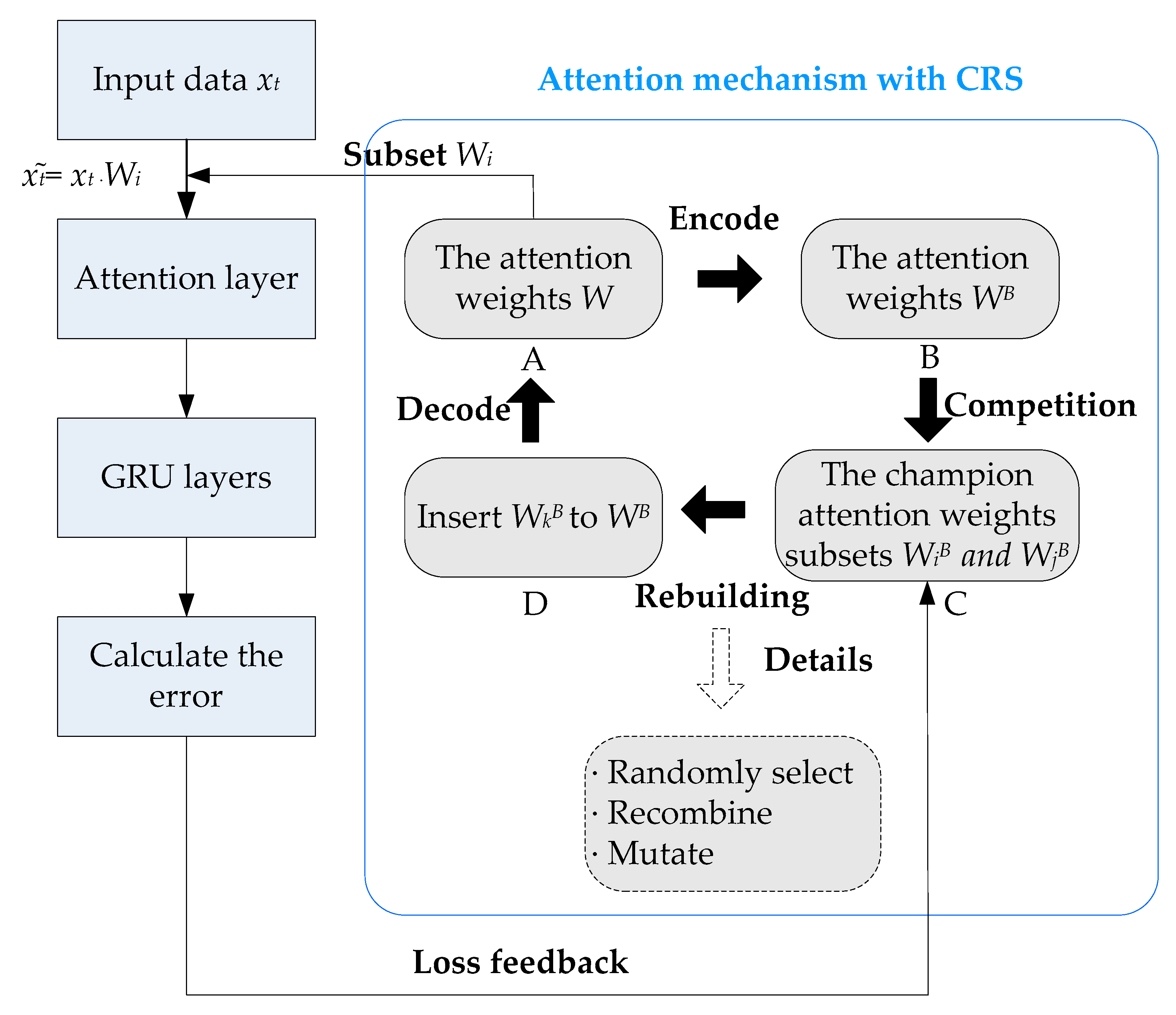
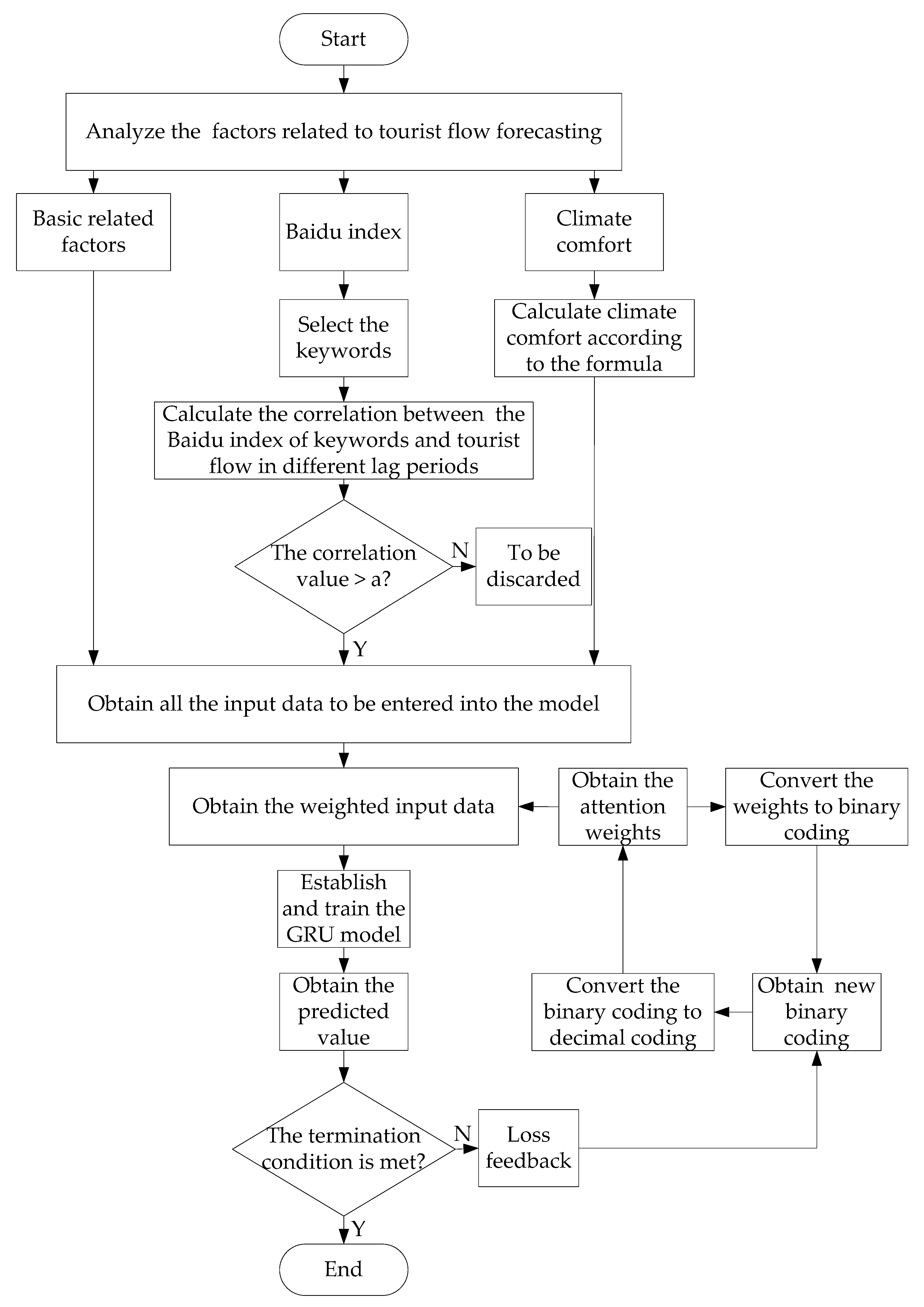
When observing a scene in the real world, humans typically focus on certain fixation point at first glance. Their attention is always concentrated on a certain part of the focus. The human visual attention mechanism is a model of resource allocation, providing different attention to different areas. The attention mechanism is proposed by imitating the principle of human vision’s attention distribution; then, the attention mechanism is combined with the encode–decode framework [22] to complete the process of attention change. The focus of this study is to assign different attention weights to different related factors through the attention mechanism and continuously optimize the weights to improve the prediction effect of the model. The attention mechanism attached to the encode–decode framework is exhibited in Figure 3 (see Section 2.4 for details).

Figure 3 illustrates how the attention mechanism is combined with the encode–decode framework. We attach attention weights $W_1$,$W_2$,…,$W_n$ to input variables $x_1$,$x_2$,…,$x_n$, transform the attention weights into intermediate semantics $C_1$,$C_2$,…,$C_n$ through encoding, and then transform the intermediate semantics into new attention weights $W_1{}^{\prime }$,$W_2{}^{\prime }$,…,$W_n{}^{\prime }$ through decoding.

2.4. IA-GRU Model

When the GRU model constructs tourist flow forecasting, the entire training process is continuously learning and memorizing the effects of various related factors on the target value. The proposed IA-GRU model in this study combines the attention mechanism with GRU. On the basis of the ability of GRU to handle time series prediction problems, the IA-GRU model assigns different attention weights to different related factors and continuously optimizes them to improve the learning and generalization abilities to achieve the purpose of improving the prediction effect of the model.

Figure 4 consists of two parts. The left part shows the process of GRU modeling and training, whereas the right part shows the process of attention mechanism with CRS to optimize attention weights. In the left part, we obtain the input data. Then, we add an attention layer to GRU on the basis of how human vision processes input information through the attention mechanism. The introduced attention mechanism can quantitatively attach weights to related factors with different importance to avoid distraction. Finally, the weighted input data is sent to the GRU layers to obtain the predicted value. The prediction error is also calculated. Moreover, the predicted errors are regarded as feedback and sent to direct the process of optimizing attention weights. In the right part, the randomly generated attention weights set is binary encoded. Then, the champion attention weights subset is selected according to the error feedback, and the new attention weights are reconstructed. Finally, the updated attention weights set is decoded, whereas the optimal attention weights are sent to the attention layer.

The concrete steps of the modeling and training of GRU and the combined attention mechanism and CRS used to optimize the attention weights are presented as follows:

(1) Modeling and training of GRU

Step 1: n columns of input data are obtained, corresponding to n related factors: $x_t=(x_t^1,x_t^2,\dots ,x_t^n)$.

Step 2: attention weights are defined: $W_i=(W_i^1,W_i^2,\dots ,W_i^n)$.

Step 3: the input data are weighed at the attention layer: ${\tilde{x}}_t=(x_t^1{W}_i^1,x_t^2{W}_i^2,\dots ,x_t^n{W}_i^n)$.

Step 4: ${\tilde{x}}_t$ is sent to GRU neural networks to acquire the final predicted value.

(2) Combined attention mechanism and CRS optimizing attention weights

According to the genetic algorithm, the purpose of CRS is to generate the optimal parameter combination in the attention layer. The process of CRS is elaborated in Figure 4. CRS comprises four parts, which are introduced as follows:

In Figure 4, attention weights set $W$ is provided in “A,” while being translated into $W^B$ through binary code in “B.” The subset $W_i$ denotes attention weights and is transferred into GRU neural networks in the left part, wherein it produces a corresponding loss value according to a predicted error in the networks. Then, the champion attention weights subsets $W_i^B$ and $W_i^B$ are selected according to the loss of $W^B$ in “C,” and its subset combination is traversed repeatedly. Finally, a new attention weight $W_k^B$ is rebuilt in “D.” The three random operators in the dotted box are introduced to illustrate how $W_k^B$ is rebuilt.

The concrete steps of CRS are stated as follows:

Step 1: attention weights set of size M = 36 are randomly generated: $W=(W_1,W_2,\dots ,W_i,\dots W_M)$.

Step 2: subset $W_i$ is sent to the attention layer, whereas $W$ is binary encoded: $W^B=(W_1^B,W_2^B,\dots ,W_i^B,\dots ,W_M^B)$.

Step 3: the prediction error is calculated based on the true value $y$ and the predicted value $\widehat{y}$ from the GRU model: $Loss(\widehat{y}(W),y)$.

Step 4: according to the error feedback, the champion attention weights subsets $W_i^B$ and $W_j^B$ are selected. Each subset comprises binary strings and is evenly divided into n segments, where n is the number of related factors mentioned in the first part of this section. Correspondingly, $W_i^B$ and $W_j^B$ are represented by $W_i^B=(F_i^1,F_i^2,\dots ,F_i^n)$ and $W_j^B=(F_j^1,F_j^2,\dots ,F_j^n)$. $F_i^1$ and $F_j^1$ are part of $W_i^B$ and $W_j^B$, respectively.

Step 5: the segments of $W_i^B$ and $W_j^B$ are randomly selected. For instance, segment n-1 of the two is selected, that is, $F_i^{n-1}$ and $F_j^{n-1}$. However, the number of selected subsections is not fixed.

Step 6: genetic recombination of $F_i^{n-1}$ and $F_j^{n-1}$ are obtained. $F_i^{n-1}$ and $F_j^{n-1}$ are represented by binary codes with a length of six, and the two are randomly exchanged on the corresponding six indices to obtain the recombined segment $F_k^{n-1}$. For example, $F_i^{n-1}=(0,1,0,0,1,1)$ and $F_j^{n-1}=(1,0,1,0,0,1)$ are exchanged on the odd index to obtain $F_k^{n-1}=(1,1,1,0,0,1)$. The indices where actual exchanges transpire are decided randomly.

Step 7: a genetic mutation is imitated and the genotype of $F_k^{n-1}$ is reversed. For instance, 0 is reversed to 1. Then, $F_k^{n-1}=(0,0,0,1,1,0)$ replaces the corresponding $F_i^{n-1}$ in $W_i^B$, forming $W_k^B$ that is inserted into $W^B$.

Step 8: $W^B$ is decoded to acquire the updated attention weights set: $W^{\prime }=(W_1{}^{\prime },W_2{}^{\prime },\dots ,W_k{}^{\prime },\dots ,W_M{}^{\prime })$.

Step 9: Steps 2–8 above should be repeated until the preset number of epochs is reached.

The entire process from the selection of input data to the training and optimization of the IA-GRU model is shown in Figure 5 (see Section 3 for concrete steps for selecting input data).

3. Data Preparation

This study takes the Huangshan Scenic Area as an example of a famous Chinese scenic spot. Huangshan is listed as one of UNESCO world natural and cultural heritage sites in 1990. Moreover, Huangshan has been selected as one of the first global geoparks in 2004. A total of 3.38 million local and foreign tourists have visited Huangshan in 2018.

In this study, we use the daily historical data of the Huangshan Scenic Area from 2014 to 2018 as experimental data. The data includes (1) Basic data: the total number of tourists in the past, target total number of tourists, number of online bookings, weather, official holiday, and weekends; (2) the Baidu index of keywords: Huangshan, Huangshan weather, Huangshan tourism guide, Huangshan tourism, Huangshan scenic area, Huangshan tickets, Huangshan first-line sky, Anhui Huangshan, Huangshan weather forecast, and Huangshan guide; (3) climate comfort: composed of average temperature, average relative humidity, and average wind speed. The data (1) is obtained from a research project in cooperation with the Huangshan scenic area. The data (2) is obtained from Baidu Index Big Data Sharing Platform (http://index.baidu.com/v2/index.html?from=pinzhuan#/). The data (3) is obtained from the China Meteorological Data Network (http://data.cma.cn/).

3.1. Basic Data

To learn as many data features and tourist flow rules as possible, the data from 2014 to 2017 were selected as the training set and the data from 2018 were selected as the test set.

(1) Total number of tourists in the past

The total number of tourists in the past is selected as one of the related factors of the prediction model, given that the annual and even daily tourist flow shows a certain regularity. The impact of past tourist flow on the current tourist flow may have a lag period. Thus, a correlation analysis was made between the past total number of tourists with different lag periods and the target total number of tourists. In this study, the maximum lag period was two years. Based on previous experience, the total number of tourists in the past with a correlation index greater than 0.440 was selected as the input variable.

Table 1. Correlation analysis results of the total number of people.

Lag Period	0	1	2	3	4	5	6	7	…
Correlation	1.000	0.718	0.443	0.324	0.243	0.197	0.256	0.341	…
Lag Period	365	366	367	368	369	370	371	372	…
Correlation	0.522	0.350	0.280	0.212	0.147	0.187	0.267	0.201	…

shows the correlation analysis results with a confidence level of 0.01.

Therefore, the total number of tourists in the past with a lag period of one day, two days, and 365 days were selected as the input variables, that is, the total number of tourists yesterday $x_1$, the total number of tourists the day before yesterday $x_2$, and the total number of tourists on the day of last year $x_3$.

(2) Number of online bookings

Given the internet’s rapid growth, its impact on people’s lifestyles is increasingly evident. Online operations are becoming persistently convenient. To a great extent, the number of online bookings can reflect the trend of the total number of tourists. Therefore, the number of online bookings was selected as the input variable $x_4$.

(3) Weather

The weather is the decisive factor for outbound tourism, wherein the weather is either good or bad for tourists. Therefore, the weather is selected as the input variable $x_5$ in the form of a dummy variable:

$x_5={{\displaystyle \{}}_1^0$, where 0 represents non-severe weather, such as sunny, cloudy, and drizzle; 1 represents severe weather, such as moderate rain, heavy rain, moderate snow, heavy snow, and blizzard.

(4) Official holiday

Traveling on holidays is a common phenomenon. Whenever a holiday arrives, the number of tourists in famous scenic spots consistently soars. Therefore, holidays were selected as input variable $x_6$ in the form of a dummy variable:

$x_6={{\displaystyle \{}}_1^0$, where 0 indicates an ordinary day; 1 indicates official holiday.

(5) Weekend

A week cycle comprises seven days. Monday to Friday is weekdays and Saturday and Sunday are rest days. Going out and traveling on rest days are common phenomena. Therefore, the weekend was selected as the input variable $x_7$ in the form of a dummy variable:

$x_7={{\displaystyle \{}}_1^0$, where 0 represents a working day; 1 represents the rest of the day.

3.2. Baidu Index of Keywords

Baidu is the largest search engine in China and has the most users. When searching for consumer behavior in China, Baidu search has higher predictive power than Google search [37]. This study selects the keywords that tourists commonly use in the Baidu search engine to search the key analysis object. We search for the keyword “Huangshan” in Baidu’s keywords-mining tool (http://stool.chinaz.com/baidu/words.aspx), and find the top-10 keywords related to Huangshan in the top 100 rankings, namely, Huangshan, Huangshan weather, Huangshan tourism guide, Huangshan tourism, Huangshan scenic area, Huangshan tickets, Huangshan first-line sky, Anhui Huangshan, Huangshan weather forecast, and Huangshan guide. Considering that the Baidu search has a lagging effect on tourist flow, a correlation analysis between the above Baidu index of keywords with different lag periods and the target total number of tourists is performed. Similarly, the maximum lag period is two years. Accordingly, the Baidu index of keywords with a correlation index greater than 0.440 is selected as input variable. The analysis results are shown in

Table 2. Correlation analysis results of the top five keywords.

lag Period	Huangshan	Huangshan Weather	Huangshan Tourism Guide	Huangshan Tourism	Huangshan Scenic Area
0	0.510	0.107	0.523	0.107	0.330
1	0.552	0.180	0.597	0.206	0.367
2	0.556	0.236	0.614	0.281	0.356
3	0.491	0.221	0.569	0.278	0.299
4	0.432	0.198	0.510	0.262	0.242
5	0.393	0.178	0.462	0.241	0.202
6	0.330	0.146	0.411	0.160	0.172
7	0.280	0.125	0.374	0.115	0.150
…	…	…	…	…	…
365	0.322	0.099	0.350	0.170	0.156
366	0.363	0.118	0.396	0.236	0.183
367	0.376	0.123	0.413	0.259	0.185
368	0.362	0.118	0.404	0.259	0.165
369	0.346	0.115	0.385	0.246	0.144
370	0.292	0.098	0.337	0.171	0.115
371	0.244	0.089	0.298	0.124	0.086
372	0.253	0.106	0.293	0.170	0.085

and

Table 3. Correlation analysis results of the last five keywords.

lag Period	Huangshan Tickets	Huangshan First-Line Sky	Anhui Huangshan	Huangshan Weather Forecast	Huangshan Guide
0	0.232	0.209	0.372	0.188	0.354
1	0.281	0.198	0.462	0.324	0.463
2	0.275	0.184	0.542	0.420	0.500
3	0.243	0.166	0.527	0.397	0.473
4	0.217	0.147	0.489	0.354	0.426
5	0.209	0.135	0.455	0.329	0.383
6	0.195	0.128	0.376	0.272	0.301
7	0.153	0.118	0.312	0.239	0.237
…	…	…	…	…	…
365	0.206	0.114	0.260	0.199	0.158
366	0.208	0.114	0.322	0.261	0.241
367	0.194	0.112	0.355	0.280	0.258
368	0.184	0.106	0.362	0.264	0.255
369	0.182	0.102	0.356	0.260	0.244
370	0.168	0.097	0.301	0.212	0.190
371	0.152	0.089	0.253	0.178	0.146
372	0.135	0.081	0.273	0.218	0.167

.

As shown in Table 2 and Table 3, the Baidu index of keyword with a lag period of two days has the highest correlation with the actual total number of tourists. Thus, we chose the Baidu index of Huangshan, Huangshan tourism guide, Anhui Huangshan, and Huangshan guide with a lag period of two days as input variables $x_8$, $x_9$, $x_{10}$, and $x_{11}$, respectively.

3.3. Climate Comfort

Climate comfort is an important environmental factor that affects tourists’ travel. Therefore, we select climate comfort as the input variable $x_{12}$. Climate comfort is the climatic condition in which people can maintain the normal physiological process and feel comfortable without any help of heat and cold [38]. The degree of human comfort is closely related to meteorological conditions, which are the comprehensive feeling of temperature, humidity, and wind in the meteorological field. The equation for calculating climate comfort is presented as follows [39]:

$$Q=1.8t-0.55(1.8t-26)(1-h)-3.25v+32.$$

(15)

In Equation (15), $t$ is the average temperature (°C), $h$ is the average relative humidity (%), $v$ is the average wind speed (m/s), and $Q$ is the climate comfort.

4. Experiments and Results

4.1. Building IA-GRU Model

In the IA-GRU model, except for the attention layer, parameters used in GRU neural networks can be learned by standard backpropagation through time algorithm with mean squared error as the objective function. According to previous experience and the results of repeated experiments, the IA-GRU model has six layers, namely, one attention layer, four GRU layers, and one fully connected layer. Moreover, the total number of neurons in four GRU layers was 128, 64, 64, and 32, respectively. The activation function of the fully connected layer is the Scaled Exponential Linear Units function. The number of training epochs in GRU layers is 500, and the mini-batch size of the training dataset is 64. According to the results of trial and error, the number of epochs in CRS was 15. Therefore, the IA-GRU model has been established in this study.

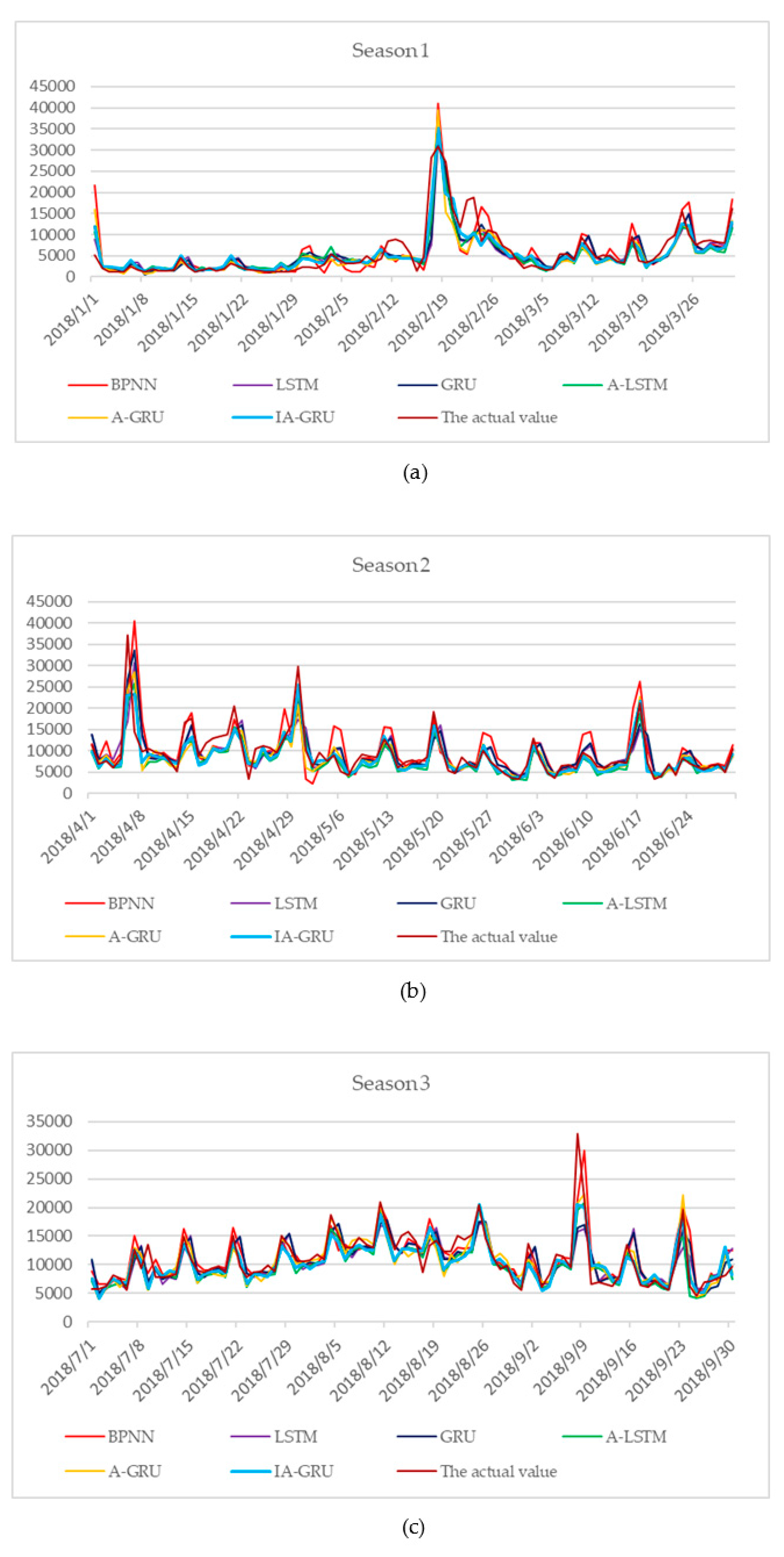
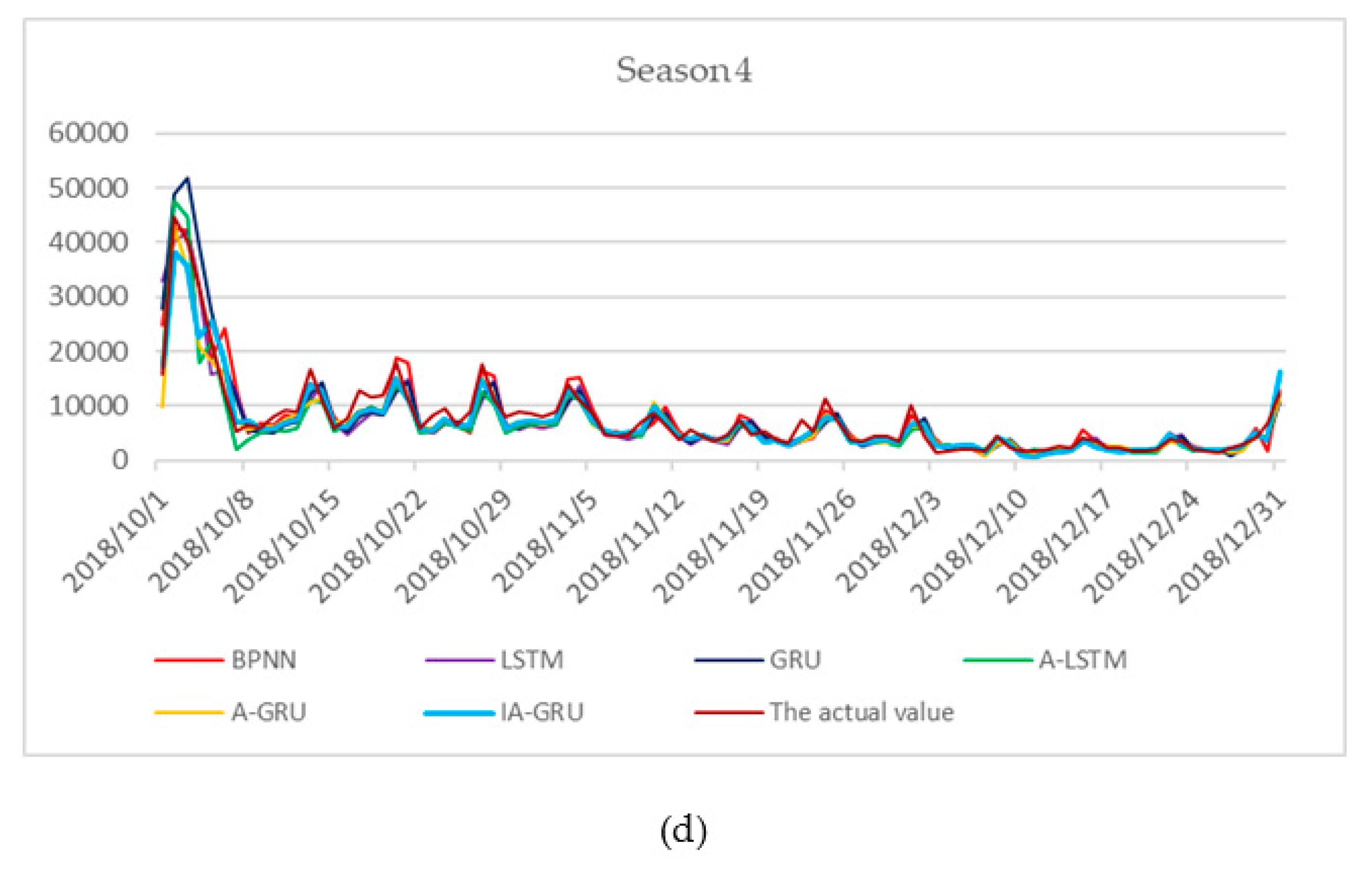
4.2. Results and Discussion

The proposed IA-GRU model is compared with some basic models, such as Back Propagation Neural Network (BPNN), LSTM, GRU, Attention-LSTM (A-LSTM), and Attention-GRU (A-GRU). The dataset of the IA-GRU model and basic models includes basic data $x_1$–$x_7$, Baidu index of keywords (1–4 keywords) $x_8$–$x_{11}$, and climate comfort $x_{12}$. To evaluate the predictive performance of each model, we choose the average absolute percentage error (MAPE) and the correlation coefficient (R) as the evaluation indicators. MAPE represents the prediction error, and R represents the degree of correlation between the predicted value and the true value. The smaller the MAPE, the smaller the deviation between the predicted value and the true value; the closer R is to 1, the higher the degree of correlation between the predicted value and the true value. The equations are presented as follows:

$$\mathrm{MAPE}=\frac{1}{\mathrm{n}}({\displaystyle \sum _{i=1}^n|\frac{y_i-{\widehat{y}}_i}{y_i}|})\times 100,$$

(16)

$$\mathrm{R}=\frac{{\displaystyle \sum _{i=1}^{\mathrm{n}}{y}_i{\widehat{y}}_i}}{\sqrt{{\displaystyle \sum _{i=1}^{\mathrm{n}}{y}_i{}^2}}\sqrt{{\displaystyle \sum _{i=1}^{\mathrm{n}}{\widehat{y}}_i{}^2}}}.$$

(17)

In the equations, $y_i$ represents the true value and ${\widehat{y}}_i$ represents the predicted value.

In this section, we apply the data $x_1$–$x_{12}$ to IA-GRU model and basic models to testify the validity of the IA-GRU model on tourist flow forecasting. The overall experimental results are shown in

Table 4. Experimental results of different models.

Models	MAPE(%)	R
IA-GRU	20.81	0.9761
A-GRU	21.71	0.9674
A-LSTM	22.87	0.9711
GRU	25.43	0.9547
LSTM	25.57	0.9480
BPNN	28.58	0.9462

, and the daily true and predicted values are shown in Figure 6. IA-GRU model with MAPE was lower than the others and R is higher than the others, which signifies that the prediction effect of the IA-GRU model is better than the abovementioned basic models. With regard to MAPE, IA-GRU was 7.77% lower than BPNN, in which MAPE was the highest. With regard to R, IA-GRU was 0.0299 higher than BPNN, in which R was the lowest. Furthermore, by comparing IA-GRU with A-GRU, we found that the former had a lower MAPE and a higher R, which indicates that the improved attention mechanism proposed in this study played a significant role. By comparing GRU with LSTM or comparing A-GRU with A-LSTM, the results show that the prediction effect of GRU was better than that of LSTM. However, R of the A-GRU model is lower than the R of the A-LSTM model. BPNN was not chosen in this area given that its MAPE was too high for forecasting at 28.58%. In summary, the IA-GRU model had the best prediction effect.

To further verify the prediction effect of the IA-GRU model, the comparative experiments in this study were divided into four categories, that is, the prediction results of different models including datasets 1, 2, 3, and 4. Dataset 1 contains basic data, dataset 2 contains basic data and Baidu index of keywords (4 keywords), dataset 3 contains basic data and climate comfort, and dataset 4 contains basic data, Baidu index of keywords, and climate comfort. Dataset 4 is the dataset mentioned in the previous paragraph.

Table 5. The results with dataset 1.

Models	MAPE(%)	R
IA-GRU	22.43	0.9736
A-GRU	24.55	0.9696
A-LSTM	25.46	0.9660
GRU	27.36	0.9494
LSTM	27.91	0.9659
BPNN	30.17	0.9460

,

Table 6. The results with dataset 2.

Models	MAPE(%)
	One Keyword	Two Keywords	Three Keywords	Four Keywords
IA-GRU	22.34	22.04	22.40	21.33
A-GRU	23.74	23.68	23.19	23.54
A-LSTM	24.59	24.38	24.09	23.89
GRU	27.16	25.86	24.99	25.54
LSTM	27.43	27.40	27.66	26.78
BPNN	29.81	29.87	29.24	28.78

,

Table 7. The results with dataset 2.

Models	R
	One Keyword	Two Keywords	Three Keywords	Four Keywords
IA-GRU	0.9677	0.9707	0.9720	0.9761
A-GRU	0.9644	0.9673	0.9713	0.9678
A-LSTM	0.9678	0.9740	0.9662	0.9736
GRU	0.9533	0.9563	0.9517	0.9532
LSTM	0.9688	0.9485	0.9724	0.9725
BPNN	0.9464	0.9397	0.9445	0.9528

,

Table 8. The results with dataset 3.

Models	MAPE(%)	R
IA-GRU	21.48	0.9688
A-GRU	22.67	0.9663
A-LSTM	23.89	0.9766
GRU	25.62	0.9538
LSTM	26.89	0.9504
BPNN	28.86	0.9542

and

Table 9. The results with dataset 4.

Models	MAPE(%)	R
IA-GRU	20.81	0.9761
A-GRU	21.71	0.9674
A-LSTM	22.87	0.9711
GRU	25.43	0.9547
LSTM	25.57	0.9480
BPNN	28.58	0.9462

exhibit the experimental results of different models including datasets 1–4. The increase in keywords in Table 6 and Table 7 is in accordance with the correlation index in Section 3.3 from high to low. The results show that more keywords make the prediction more accurate. As shown in Table 5, Table 6, Table 7, Table 8 and Table 9, the prediction effect of IA-GRU model is better than the other basic models on each dataset, wherein the predicted value had a higher correlation with the real value. In the four datasets, the IA-GRU model had the lowest MAPE on dataset 4 and the highest R, which signifies that the Baidu index of keywords and climate comfort further improve prediction accuracy.

To further analyze the prediction accuracy of the IA-GRU model, we performed a monthly analysis of the experimental results of different models using dataset 4, as shown in

Table 10. The monthly analysis results with dataset 4.

Months	MAPE(%)
	IA-GRU	A-GRU	A-LSTM	GRU	LSTM	BPNN
1	40.86	32.38	48.92	41.85	40.28	51.30
2	30.73	35.58	38.16	37.47	35.41	46.67
3	25.82	27.82	23.95	29.35	29.18	32.32
4	23.26	26.88	26.95	27.97	30.16	29.25
5	13.72	17.56	17.67	21.45	23.44	33.58
6	14.25	14.27	15.84	18.7	18.34	24.52
7	12.53	14.51	13.27	14.86	16.96	13.55
8	13.38	13.36	11.94	11.71	11.74	11.16
9	18.51	17.03	18.25	23.60	24.48	26.94
10	18.27	17.62	23.14	29.84	30.13	28.15
11	14.17	16.26	16.68	18.11	21.62	21.22
12	24.82	28.24	20.74	30.93	25.79	25.63
Average	20.81	21.71	22.87	25.43	25.57	28.58

and

Table 11. The monthly analysis results with dataset 4.

Months	R
	IA-GRU	A-GRU	A-LSTM	GRU	LSTM	BPNN
1	0.9538	0.8650	0.9502	0.9132	0.9506	0.8226
2	0.9546	0.9219	0.9443	0.9270	0.9226	0.8804
3	0.9779	0.9751	0.9803	0.9554	0.9498	0.9585
4	0.9673	0.9447	0.9557	0.9309	0.9070	0.9054
5	0.9880	0.9808	0.9823	0.9648	0.9581	0.9348
6	0.9915	0.9895	0.9917	0.9698	0.9682	0.9788
7	0.9845	0.9810	0.9852	0.9764	0.9723	0.9878
8	0.9912	0.9890	0.9938	0.9913	0.9912	0.9918
9	0.9685	0.9709	0.9675	0.9390	0.9319	0.9496
10	0.9860	0.9875	0.9750	0.9718	0.9580	0.9725
11	0.9842	0.9802	0.9806	0.9714	0.9609	0.9685
12	0.9549	0.9582	0.9663	0.9402	0.9459	0.9529
Average	0.9761	0.9674	0.9711	0.9547	0.9480	0.9462

. As shown in Table 10, the annual average error of the IA-GRU model was lower than that of basic models, whereas the error of all models from May to October is lower than the annual average error. In May, June, and July, the error of the IA-GRU model was lower than that of basic models. All models exhibited high errors in January, February, March, April, and December. One of the reasons may be that they were in the off-peak period. Moreover, the actual value is small, which is likely to cause high numerical deviations. Overall, the IA-GRU model is relatively stable. In February, April, May, June, July, and November, the IA-GRU model had the lowest error. Although the prediction of the IA-GRU model was not the best in other months of the year, it was not the worst. For example, the error in January was 8.48% higher than the minimum error, but 10.44% lower than the maximum error. The errors in March, September, and October were close to the minimum error, wherein the gap between the error and the minimum error in these three months is less than 2%. The performance of IA-GRU model in December was similar to that in January. IA-GRU model had the largest error in August, which was 2.22% higher than the lowest error. In August, the gap between the two errors is relatively small. The reason may be that a certain gap exists in the correlation index of the Baidu index between the training and test sets. Through correlation analysis, as shown in

Table 12. Correlation analysis results of keywords in August.

	Huangshan	Huangshan Travel Guide	Anhui Huangshan	Huangshan Guide
Training set	0.295	0.445	0.225	0.275
Test set	0.478	0.656	0.061	0.321

, we find that the correlation index of the Baidu index of the training set is low, but the correlation index of the Baidu index of the test set is high, which may cause a certain bias in the feature learning of the Baidu index. As shown in Table 11, the R of the IA-GRU model was the highest in January, February, April, May, and November, and the R from January to December was greater than 0.95. Such values are closely related to the annual average R. Thus, the IA-GRU model was relatively stable, compared to other models.

In summary, the proposed IA-GRU model based on the Baidu index and climate comfort can effectively improve the accuracy of tourist flow forecasting. Moreover, the model proposed in this study is generally better than other basic models, proving the effectiveness of the model in tourist flow forecasting.

5. Conclusions

This study proposes IA-GRU model trained with CRS for accurate tourist flow forecasting. Tourism is an important part of the local, national, and global economies. Thus, good predictive models are becoming increasingly valuable in tourist destinations management. First, this study is the first to apply GRU in the field of tourist flow forecasting, wherein an attention layer is added into GRU neural networks. Then, an improved attention mechanism that weighs different related factors is proposed. Finally, the improved attention mechanism is combined with GRU, and CRS is used to generate the optimal parameter combination at the attention layer. As a result, the IA-GRU model captures long-term dependencies and increases the degree of attention that GRU pays to the characteristics of sub-windows in different related factors. Concurrently, this study also explores the application of the Baidu index and climate comfort in prediction models. In selecting the Baidu index of keywords, Baidu’s keywords-mining tools and correlation analysis methods are used to screen out relevant keywords with a large correlation index. In synthesizing climatic comfort, the comprehensive sensation of temperature, humidity, and wind speed in the meteorological field is considered, and the corresponding climatic comfort is calculated. This study takes the famous Huangshan Scenic Area as an example to verify the effectiveness of the IA-GRU model with the Baidu index and climate comfort in tourist flow forecasting. The experimental results prove that the IA-GRU model with the Baidu index and climate comfort has higher prediction accuracy in tourist flow forecasting than basic models. Thus, the proposed model can help the administration department in managing the scenic area efficiently. Although this study has certain limitations, it remains worthy of further study in the future. For example, a more detailed method of dividing weather dummy variables, a more accurate method of keywords selection, and a more accurate method of climate comfort calculation can be explored in future studies. In general, the proposed IA-GRU model is highly suitable for tourist flow forecasting. Overall, the proposed model provides a significant reference for tourist destinations management and a new perspective for related research.

References

1. Wang, J. Anhui Statistical Yearbook; China Statistics Publishing House: Beijing, China, 2017. [Google Scholar]
2. Li, G.; Song, H.; Witt, S.F. Recent developments in econometric modeling and forecasting. J. Travel Res. 2005, 44, 82–99. [Google Scholar] [CrossRef] [Green Version]
3. Burger, C.; Dohnal, M.; Kathrada, M.; Law, R. A practitioners guide to time-series methods for tourism demand forecasting—A case study of Durban, South Africa. Tour. Manag. 2001, 22, 403–409. [Google Scholar] [CrossRef]
4. Croes, R.R.; Vanegas, M., Sr. An econometric study of tourist arrivals in Aruba and its implications. Tour. Manag. 2005, 26, 879–890. [Google Scholar] [CrossRef]
5. Daniel, A.C.M.; Ramos, F.F. Modelling inbound international tourism demand to Portugal. Int. J. Tour. Res. 2002, 4, 193–209. [Google Scholar] [CrossRef]
6. Witt, S.F.; Song, H.; Wanhill, S. Forecasting tourism-generated employment: The case of denmark. Tour. Econ. 2004, 10, 167–176. [Google Scholar] [CrossRef]
7. Chu, F.-L. Forecasting tourism demand with ARMA-based methods. Tour. Manag. 2009, 30, 740–751. [Google Scholar] [CrossRef]
8. Gil-Alana, L. Modelling international monthly arrivals using seasonal univariate long-memory processes. Tour. Manag. 2005, 26, 867–878. [Google Scholar] [CrossRef]
9. Chen, C.-F.; Chang, Y.-H.; Chang, Y.-W. Seasonal ARIMA forecasting of inbound air travel arrivals to Taiwan. Transportmetrica 2009, 5, 125–140. [Google Scholar] [CrossRef]
10. Chen, K.-Y.; Wang, C.-H. Support vector regression with genetic algorithms in forecasting tourism demand. Tour. Manag. 2007, 28, 215–226. [Google Scholar] [CrossRef]
11. Hong, W.-C.; Dong, Y.; Chen, L.-Y.; Wei, S.-Y. SVR with hybrid chaotic genetic algorithms for tourism demand forecasting. Appl. Soft Comput. 2011, 11, 1881–1890. [Google Scholar] [CrossRef]
12. Benardos, P.; Vosniakos, G.-C. Optimizing feedforward artificial neural network architecture. Eng. Appl. Artif. Intell. 2007, 20, 365–382. [Google Scholar] [CrossRef]
13. Law, R.; Au, N. A neural network model to forecast Japanese demand for travel to Hong Kong. Tour. Manag. 1999, 20, 89–97. [Google Scholar] [CrossRef]
14. Law, R. Back-propagation learning in improving the accuracy of neural network-based tourism demand forecasting. Tour. Manag. 2000, 21, 331–340. [Google Scholar] [CrossRef]
15. Hochreiter, S.; Schmidhuber, J. Long short-term memory. Neural Comput. 1997, 9, 1735–1780. [Google Scholar] [CrossRef] [PubMed]
16. Cho, K.; Van Merriënboer, B.; Bahdanau, D.; Bengio, Y. On the properties of neural machine translation: Encoder-decoder approaches. arXiv 2014, arXiv:1409.1259. [Google Scholar]
17. Cho, K.; Van Merriënboer, B.; Gulcehre, C.; Bahdanau, D.; Bougares, F.; Schwenk, H.; Bengio, Y. Learning phrase representations using RNN encoder-decoder for statistical machine translation. arXiv 2014, arXiv:1078.1406. [Google Scholar]
18. Soltau, H.; Liao, H.; Sak, H. Neural speech recognizer: Acoustic-to-word LSTM model for large vocabulary speech recognition. arXiv 2016, arXiv:09975.1610. [Google Scholar]
19. Zheng, H.; Yuan, J.; Chen, L. Short-term load forecasting using EMD-LSTM neural networks with a Xgboost algorithm for feature importance evaluation. Energies 2017, 10, 1168. [Google Scholar] [CrossRef] [Green Version]
20. Mujeeb, S.; Javaid, N.; Ilahi, M.; Wadud, Z.; Ishmanov, F.; Afzal, M.K. Deep long short-term memory: A new price and load forecasting scheme for big data in smart cities. Sustainability 2019, 11, 987. [Google Scholar] [CrossRef] [Green Version]
21. Li, Y.; Cao, H. Prediction for tourism flow based on LSTM neural network. Proced. Comput. Sci. 2018, 129, 277–283. [Google Scholar] [CrossRef]
22. Bahdanau, D.; Cho, K.; Bengio, Y. Neural machine translation by jointly learning to align and translate. arXiv 2014, arXiv:0473.1409. [Google Scholar]
23. Cho, K.; Courville, A.; Bengio, Y. Describing multimedia content using attention-based encoder-decoder networks. IEEE Trans. Multimed. 2015, 17, 1875–1886. [Google Scholar] [CrossRef] [Green Version]
24. Qin, Y.; Song, D.; Chen, H.; Cheng, W.; Jiang, G.; Cottrell, G. A dual-stage attention-based recurrent neural network for time series prediction. arXiv 2017, arXiv:02971.1704. [Google Scholar]
25. Liang, Y.; Ke, S.; Zhang, J.; Yi, X.; Zheng, Y. GeoMAN: Multi-level Attention Networks for Geo-sensory Time Series Prediction. In Proceedings of the IJCAI, Stockholm, Sweden, 13–19 July 2018; pp. 3428–3434. [Google Scholar]
26. Kim, S.; Hori, T.; Watanabe, S. Joint CTC-Attention Based End-to-End Speech Recognition Using Multi-Task Learning. In Proceedings of the 2017 IEEE International Conference on Acoustics, Speech and Signal Processing (ICASSP), New Orleans, LA, USA, 5–9 March 2017; pp. 4835–4839. [Google Scholar]
27. Zhou, H.; Zhang, Y.; Yang, L.; Liu, Q.; Yan, K.; Du, Y. Short-term photovoltaic power forecasting based on long short term memory neural network and attention mechanism. IEEE Access 2019, 7, 78063–78074. [Google Scholar] [CrossRef]
28. Wang, S.; Wang, X.; Wang, S.; Wang, D. Bi-directional long short-term memory method based on attention mechanism and rolling update for short-term load forecasting. Int. J. Electr. Power Energy Syst. 2019, 109, 470–479. [Google Scholar] [CrossRef]
29. Ran, X.; Shan, Z.; Fang, Y.; Lin, C. An LSTM-based method with attention mechanism for travel time prediction. Sensors 2019, 19, 861. [Google Scholar] [CrossRef] [Green Version]
30. Li, Y.; Zhu, Z.; Kong, D.; Han, H.; Zhao, Y. EA-LSTM: Evolutionary attention-based LSTM for time series prediction. Knowl. Based Syst. 2019, 181, 104785. [Google Scholar] [CrossRef] [Green Version]
31. Yi, S.; Benfu, L. A review of researches on the correlation between internet search and economic behavior. Manag. Rev. 2011, 23, 72–77. [Google Scholar]
32. Choi, H.; Varian, H. Predicting the present with Google trends. Econ. Record 2012, 88, 2–9. [Google Scholar] [CrossRef]
33. Bangwayo-Skeete, P.F.; Skeete, R.W. Can Google data improve the forecasting performance of tourist arrivals? Mixed-data sampling approach. Tour. Manag. 2015, 46, 454–464. [Google Scholar] [CrossRef]
34. Önder, I.; Gunter, U. Forecasting tourism demand with google trends for a major European city destination. Tour. Anal. 2016, 21, 203–220. [Google Scholar] [CrossRef]
35. Li, H.; Goh, C.; Hung, K.; Chen, J.L. Relative climate index and its effect on seasonal tourism demand. J. Travel Res. 2018, 57, 178–192. [Google Scholar] [CrossRef]
36. Chen, R.; Liang, C.-Y.; Hong, W.-C.; Gu, D.-X. Forecasting holiday daily tourist flow based on seasonal support vector regression with adaptive genetic algorithm. Appl. Soft Comput. 2015, 26, 435–443. [Google Scholar] [CrossRef]
37. Yang, X.; Pan, B.; Evans, J.A.; Lv, B. Forecasting Chinese tourist volume with search engine data. Tour. Manag. 2015, 46, 386–397. [Google Scholar] [CrossRef]
38. Stathopoulos, T.; Wu, H.; Zacharias, J. Outdoor human comfort in an urban climate. Build. Environ. 2004, 39, 297–305. [Google Scholar] [CrossRef]
39. Liang, C.; Bi, W. Seasonal Variation Analysis and SVR Forecast of Tourist Flows During the Year: A Case Study of Huangshan Mountain. In Proceedings of the 2017 IEEE 2nd International Conference on Big Data Analysis (ICBDA), Beijing, China, 10–12 March 2017; pp. 921–927. [Google Scholar]
Figure 1. Structure of long short-time memory neural network (LSTM).
Sustainability 12 01390 g001
Figure 2. Structure of Gated Recurrent Unit (GRU).
Sustainability 12 01390 g002
Figure 3. Attention mechanism.
Sustainability 12 01390 g003
Figure 4. GRU training process based on attention mechanism with competitive random search (CRS).
Sustainability 12 01390 g004
Figure 5. The flowchart.
Sustainability 12 01390 g005
Figure 6. The actual and predicted values of 2018. (a) The actual and predicted values of season 1; (b) the actual and predicted values of season 2; (c) the actual and predicted values of season 3; (d) the actual and predicted values of season 4.
Sustainability 12 01390 g006aSustainability 12 01390 g006b