Benchmarking Energy Use at University of Almeria (Spain)

Abstract

Several factors impact the energy use of university campus buildings. This study aims to benchmark the energy use in universities with Mediterranean climates. The University of Almeria campus was used as a case study, and different types of buildings were analyzed. The second goal was to model the electricity consumption and determinate which parameter correlate strongly with energy use. Macro-scale energy consumption data during a period of seven years were gathered alongside cross-sectional buildings information. Eight years of daily outdoor temperature data were recorded and stored for every half hour. This dataset was eventually used to calculate heating and cooling degree-days. The weather factor was recognized as the variable with the greatest impact on campus energy consumption, and as the coefficient indicated a strong correlation, a linear regression model was established to forecast future energy use. A threshold of 8 GWh has been estimated as the energy consumption limit to be achieved despite the growth of the university. Finally, it is based on the results to inform the recommendations for decision making in order to act effectively to optimize and achieve a return on investment.

1. Introduction

Fuel constraints are a relevant issue in both industrialized and developing countries and are related to energy prices and accessibility of energy services [1]. Public buildings such as universities, schools. and hospitals are challenged to manage the exponential growth of their energy demand and transform their buildings into energy efficient ones. The design of buildings should logically be adapted to the lowest energy consumption levels, but in most cases, it is necessary to focus on existing buildings [2]. Therefore, the reduction of both energy consumption and CO₂ emissions from buildings is one of society’s main targets today [3]. In Spain, there is a climatic classification according to the technical code of the building that contemplates these issues, which has been mandatory since 2006 [4]. Acting as models for communities, universities are supposed to provide innovative solutions through research in order to support the sustainability and reduce the carbon footprint [5]. One of the key operating aspect for universities is related to enhance students and teachers comfort levels, which may have a significant effect on their performance [6]. Visual, acoustic, and thermal comforts should not be considered as luxuries but rather as basic standard for schools [7]. However, maintaining indoor quality will eventually lead to a significant growth of electricity consumption; therefore, transforming university locals into energy efficient ones is a necessity. To ensure that these locals have optimal energy performance, researchers and professionals have developed management systems such as energy benchmarking and energy audit [8].

The energy benchmarking technique allows us to compare the energy consumption of buildings by dividing the key performance metric by gross floor area [9]; this index is usually expressed in (kBtu/ft²/yr or kWh/m²/yr), and it is labeled as Energy Use Intensity (EUI) or Energy Intensity (EI). This gives the opportunity to the portfolio manager to track the key performance metric overtime [8]. EUI is expressed as energy per square meter per year. It is calculated by dividing the total energy consumed by the building in one year by the total gross floor area of the building. The main benefit of using EUI is that the performance of a building can be compared with similar buildings across the country. EUI can vary significantly depending on building type; therefore, it is necessary to calculate it in buildings used in which there is no data so far. Energy audit is a tool that allows building owners and managers to determine which energy efficiency measures meet their sustainability goals and their investment return criteria [10]. The energy efficiency directive (201/27/EU) requires the auditing of the energy performance of old schools to assess them and propose future retrofitting if necessary [11]. In Italy, over 28% of schools are energy inefficient [12]. A previous experiment executed an energy management program in a high school located in Dubai, UAE [13], and its results show that energy performance can be basically improved by 35%. Many evaluation programs for green schools have been designed to assess managers towards sustainable solutions, like the program whole-school approaches, this initiative integrated different elements of school life such as governance, pedagogical methods, curriculum, resource management, school operations and grounds [14]. In the case of the University in Spain, particular studies have been carried out for the Universidad Politecnica de Valencia (UPV) in order to predict electricity consumption patterns in buildings [15] or the use of algorithms using demand and generation forecasts and costs of the available resources, so the benefit obtained in a whole year is five times higher, with a percentage of participation in demand response programs (DRPs), which is accepted as 60.27% or higher [16]. At this same university, with the use of energy efficiency measures (EEMs), in three different types of buildings (a research building (Building 8G), a teaching and staff building (School of Telecom Engineering building 4P), and a greenhouse building 8I-8J), the savings representing about 10% of total annual energy consumption [17].

HVAC and lighting systems have drastically changed in the last decade. Today, they incorporate sophisticated sensors and computer networking programs to monitor and adjust building systems and energy usage. These new technologies are called building automation systems, and they control, monitor, and collect data on the buildings performance technology [18,19]. University campuses serve different functions by providing spaces such as teaching rooms, academic offices, laboratories, restaurants, and sport facilities. This research outlines the classification of categories by their ECs and EUIs. The building category that influences substantially the overall EC of the University by 47% even though it covers only 27% of its total GFA. This category is the science and research category, and it is also the most energy intense by an average EUI 119.5 kWh. Similar results were reported by a study that was ran to support the ASHRAE standard 100. It has determined the EUI median for 18 major categories by climate zone in the USA, according to CBECS 2003. The national median of the laboratory has the highest energy intensity on a university campus (98 kWh/m²). Our case study provides an opportunity to treat a diverse dataset of buildings. A study carried out in Australia reported that laboratory energy intensity was the highest among other categories, and it was three times higher than non-laboratory buildings [20]. In addition, another study divided laboratories into different classes of science, applied science, and intervention, and the results show that the HVAC and electric appliances load, as well as the long operating hours, are the main reasons behind the high energy consumption of this category [21].

The quantity of energy used in universities can change from a country to another, as a recent study in Taiwan has demonstrated that gross domestic product (GDP) of the country has a positive correlation with the energy consumption [22]. Furthermore, a study carried out by Catherine and Byrne et al., (2014) summarized the major factors that significantly impact university buildings’ energy use are as follows: occupancy rate, HVAC load and artificial lighting, number of computers and electric equipment, and weather conditions [23]. The influence of these various parameters on the energy use and their correlated relationship to each other define the stochastic nature of the EC. This paper focused on two parameters—weather and the size of the active network inside the campus. The choice of those variables was made based on an energy survey that was conducted inside the campus and the analysis of energy consumption patterns over the last eight years. Unlike many previous studies that focused on modeling the occupant behavior and its influence on the EC, this study tested the impact of the network on a yearly basis. We gathered the number of occupants active inside the university, including the number of students, professors, and administrative staff, and since this parameter varies during the academic year, we had to line up the two other parameters in order to have them all on the same sequence. Then, we tested the correlation with both variables (the number of occupants and the sum of CDD and HDD) with macro-scale energy data. On the other hand, energy benchmarking seeks to give a reference value by defining reliable indicators, we split the buildings portfolio by the following six categories: research, administration office, teaching and seminary room, library, sport facility, and restaurants. This will allow us to benchmark within the same category and identify the benchmark value of each category. These values could be used in the future to define a national baseline for universities or in the Mediterranean region. As the majority of studies have proven that outdoor conditions are the main variable that influences energy use, in this study, we will test the correlation of the total EC with the size of network from one side and with the sum total of the HDD and CDD during each academic year. Moreover, identifying the variable that has the strongest correlation is primarily in order to take suitable actions to achieve better energy management.

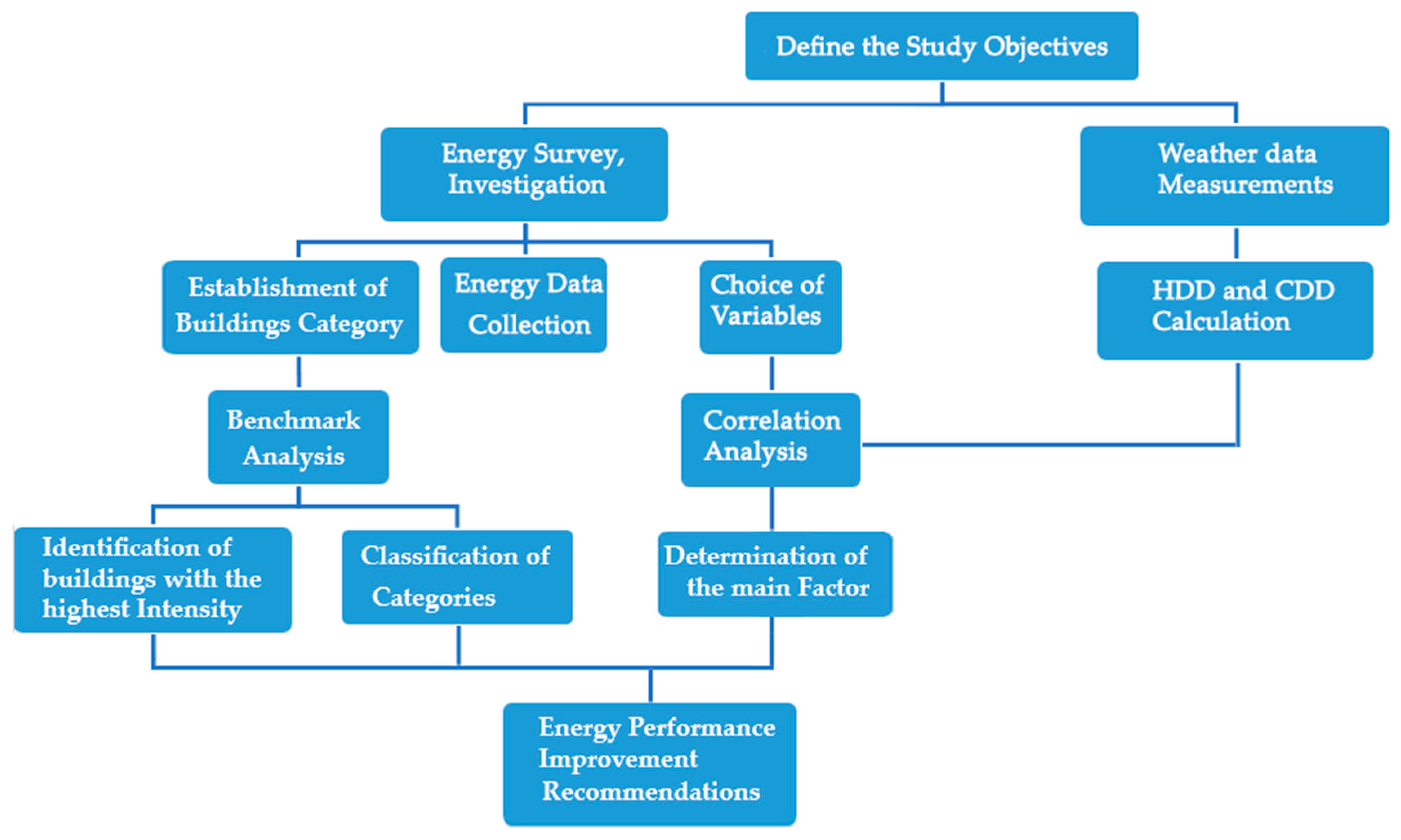
2. Materials and Methods

The University of Almeria is a Spanish Public University located in the south coast of Spain, with the coordinates of latitude 36°49′45″N and longitude −2°24′16″E, see Appendix A. The university campus spreads on a surface of 17 hectares and has 33 buildings (see Figure 1). In the 2018–2019 academic year, the university offered 38 different degree programs, with 883 lecturers and 13,547 students.

Almeria is a coastal city located on the southern region of Spain, the climate is particularly arid and semi-continental, with relatively dry warm winters with an average temperature at 16°C (60 °F) and hot summer with an average temperature of 28°C (80 °F). The most daily sunshine hours are scored in July and the wettest month is January with an average of 30mm of rain and an annual average percentage of humidity of 61.0% [24,25].

The dataset used in this analysis consists of (1) daily outdoor temperature scored every half hour during the last eight years, (2) Total energy consumption on a monthly basis and gross floor area data from 2011–2018 (

Table 1. Monthly evolution in energy consumption of the university campus per year.

Campus Monthly EC (kWh)
Month/Year	2011	2012	2013	2014	2015	2016	2017	2018
January	722,623	717,867	706,880	708,499	765,785	702,918	773,539	770,454
February	689,088	746,940	672,895	657,712	737,049	693,787	652,036	725,147
March	729,218	685,622	681,843	689,979	728,747	666,108	706,072	716,676
April	573,686	571,444	630,393	597,792	640,762	644,299	580,052	680,127
May	700,648	687,262	644,661	667,437	717,944	672,034	713,215	730,265
June	762,909	765,368	656,218	696,597	798,527	761,444	936,273	740,233
July	737,705	724,290	707,900	703,602	877,181	776,462	801,608	704,690
August	550,274	527,979	487,813	513,183	597,359	545,341	617,208	608,966
September	760,301	6933	731,827	753,425	785,407	837,467	821,574	645,724
October	693,375	654,832	727,983	710,872	721,047	742,409	780,345	699,640
November	640,273	632,938	647,683	671,644	623,533	685,437	705,548	757,993
December	621,586	629,833	627,630	683,565	616,653	645,593	691,188	872,744

), (3) campus buildings’ energy consumption data during the last three years 2016–2018 (

Table 2. Space category, energy consumption, and gross floor area.

Space Category	Building	EC (kWh/year)			GFA (m2)
		2016	2017	2018
Administration Office	1	226,192	220,042	239,366	5880
	2	329,354	331,988	320,119	11,430
	18	64,759	63,880	62,840	2620
	19	196,189	208,161	188,432	8290
	20	64,553	56,955	56,261	2450
	21	104,633	129,335	122,294	4605
	8	141,530	143,240	144,591	3994
Teaching and Seminary Room	3	300,566	330,608	327,658	5585
	5	120,802	137,864	142,172	5611
	15	107,047	119,255	123,319	4118
	12	137,493	161,042	152,614	6016
	4	13,273	13,938	16,132	12
	23	156,424	168,703	151,046	6,605
	27	296,197	362,304	369,768	8,618
	11	68,441	59,409	51,887	3,089
Research Building	9	176,596	178,167	156,995	5487
	30	812,983	809,544	842,943	4301
	28	388,289	384,574	361,428	4828
	29	734,370	788,962	796,318	4975
	16	156,650	186,889	150,348	2100
	31	294,533	246,824	199,478	1072
	24	280,959	465,018	478,491	3089
	13	735,213	767,650	691,523	12,341
Library Building	26	905,166	19,215	947,826	16,194
	32	2311	213,344	202,611	2026
Sports Facilities	10	257,182	155,856	306,779	5548
	7	89,013	76,623	78,963	3280
	17	49,892	38,184	32,967	547
Restaurant Buildings	33	42,169	41,811	61,249	1190
	6	43,690	52,910	62,919	1280

), (4) the average EUI within each category (

Table 3. Average energy use index per year and average energy consumption of each space category.

Building Category	Average EUI (kWh/m2 ·Year)	EC (kWh)
Research	119.50	3,694,915
Library	82.67	1,169,721
Sport facilities	47.30	361,820
Restaurant	41.11	101,583
Teaching and seminary	28.99	1,295,988
Administration Office	28.78	1,38,239
Others	-	28,007
Public Lighting	-	416,812

), (5) Building energy performance classification of all the buildings by category (

Table 4. Building energy performance classification of all the buildings by category.

Building Category	Energy Performance Classification
	Poor Practice <===> Best Practice
Research	31	30	29	24	16	28	13	9
Library	32	26	-	-	-	-	-	-
Sport facilities	17	10	7	-	-	-	-	-
Restaurant	6	33	-	-	-	-	-	-
Teaching and seminary	3	4	27	15	12	23	5	11
Administration Office	1	8	2	21	18	20	19	-

), the number of students, professors, and administration staff per academic year (

Table 5. Inputs and outputs used for the correlation analysis and regression model.

Academic Year	CDD & HDD (°C)	N of Occupants	N of Staff		EC (kWh)
			N of Professors	N of Administrative Staff
2011–2012	1456.30	15,062	475	806	8,142,307
2012–2013	1225.90	14,978	476	698	7,799,209
2013–2014	1091.20	15,234	477	732	7,969,924
2014–2015	1449.40	15,295	475	752	8,682,860
2015–2016	1220.40	15,417	468	791	8,209,033
2016–2017	1398.80	15,392	464	780	8,690,909
2017–2018	1417.70	15,680	468	809	8,675,213
2018–2019	1664.20	15,166	482	883	8,453,842

). Figure 2 outlines the methodology flow chart, starting from defining objectives to collecting data to developing results.

Correlation Approach

There is a lack of data for most of the electric components and the physical characteristics of the university buildings (building materials, building geometric sizes). Thus, the given data set of observations gives us the opportunity to establish a statistical approach that allows us to measure the relationship between two variables by defining there correlation coefficient, which will provide us with a straightforward interpretation of the two variables on the overall electricity consumption on a yearly basis. This method relies on historic values of overall energy consumption and background knowledge of the input variables that influence perception. In this case study, we define the first explanatory variable occupancy rate as the total number of students, professors, and administration staff for the academic year. If we get a weak correlation, we proceed by dividing the number of occupants into two groups, students and staff (professors and administration staff), and then test them separately. The second explanatory variable is the weather explanatory variable, defined as the sum of the heating and cooling degree-days during one academic year; its unit is in degrees Celsius.

Heating and cooling degree-days (HDD and CDD) are defined as the differences between the average daily outdoor temperature T(o/d) and corresponding base temperatures Tb [26]. The base temperature for heating and cooling is different from place to place. It also depends on the type of building (household, administration, hospital). In this case study, the CDD temperature base is ($\mathrm{T}\left(\mathrm{b},\mathrm{CDD}\right)$ = 28 °C) and the HDD temperature base is ($\mathrm{T}\left(\mathrm{b},\mathrm{HDD}\right)$ = 14 °C). These assumptions are based on a survey conducted inside the campus [24,25]. Note that the temperature base values indicate the outside temperature, and there is usually a minimum of two degrees of difference between the inside and outside temperatures. We sum up both variables on a sequence of every academic year so that it can be lined up with the quantity of interest (EC).

$$\mathrm{CDD}=\mathrm{T}\left(\mathrm{o}/d\right)-T\left(\mathrm{b},\mathrm{CDD}\right)\mathrm{if}T\left(\mathrm{b},\mathrm{CDD}\right)> T\left(\mathrm{o}/d\right)\mathrm{then}\mathrm{CDD}=0$$

(1)

$$\mathrm{HDD}= T\left(\mathrm{b},\mathrm{HDD}\right) - \mathrm{T}\left(o/d\right)\mathrm{if}T\left(\mathrm{b},\mathrm{HDD}\right)<T\left(\mathrm{o}/\mathrm{d}\right)\mathrm{then}\mathrm{HDD}=0$$

(2)

The extensive weather data set will be used in this paper to develop and validate statistical models. The complex nature of EC inside buildings and the lack of the data of most components of buildings drive us to a black box model that relies on a simple input and output system [27]. The statistical model of the linear regression is set up according to the Formula (3):

$$Ei=b\times \left(Xi\right)+a$$

(3)

where Ei is the annual energy consumption corresponding to the academic year i, the input Xi is the explanatory variable, b is the slope, a is the y-intercept [28].

3. Results

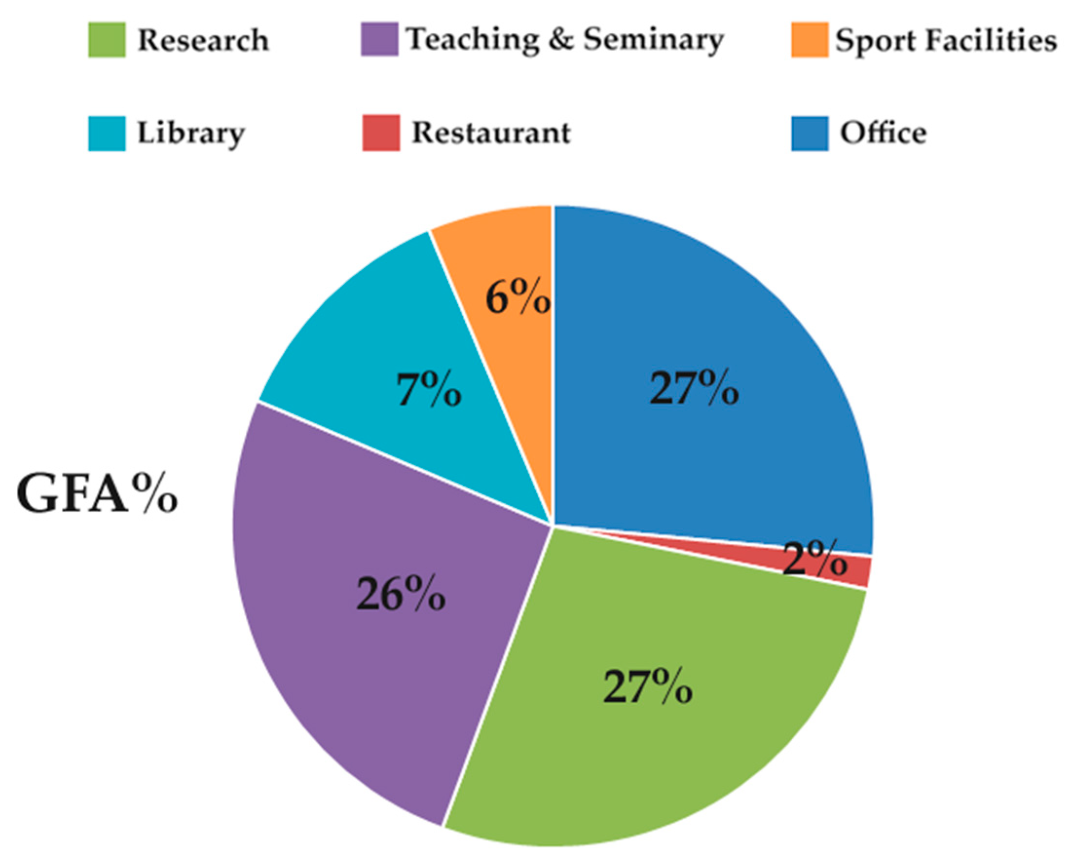
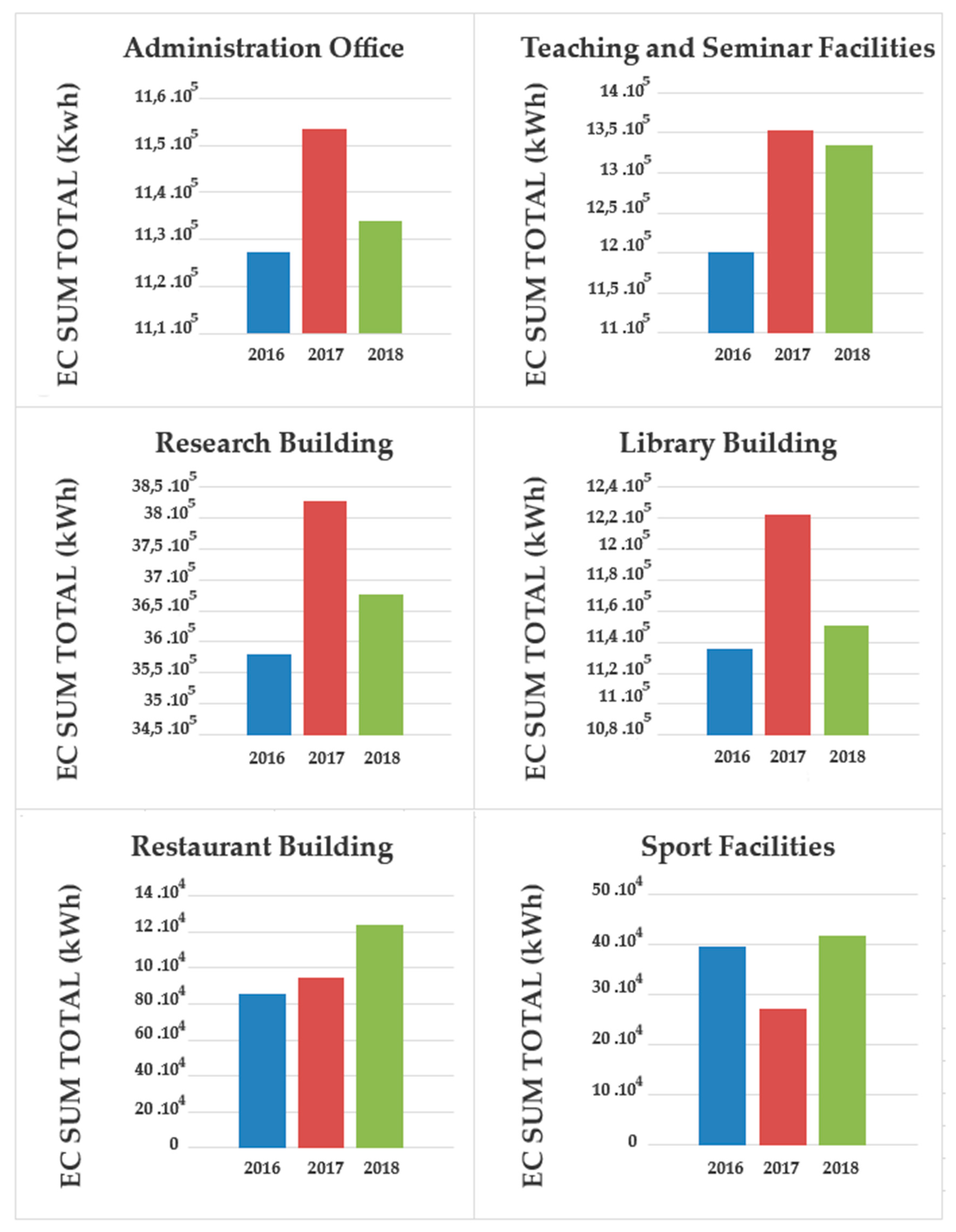
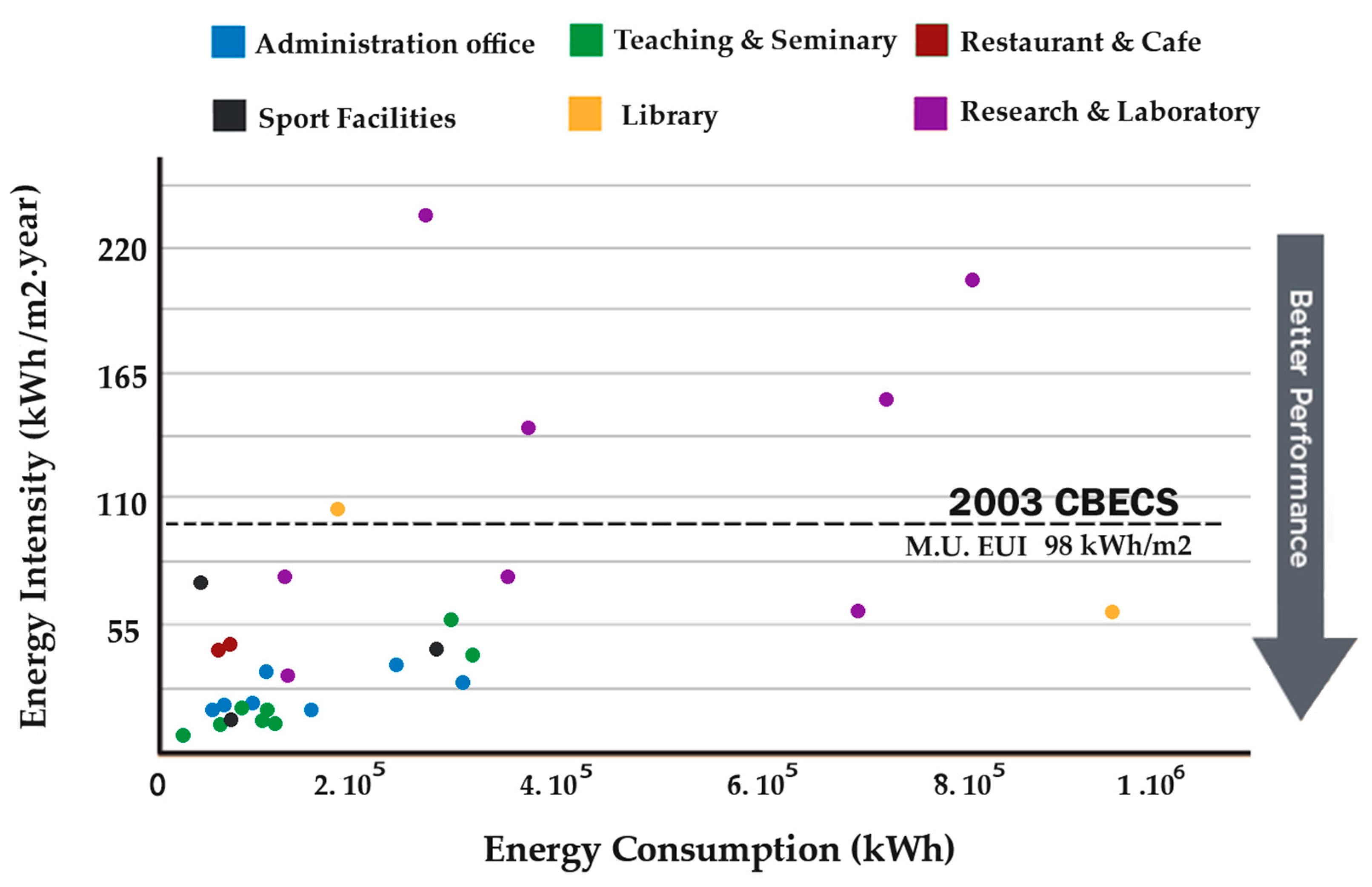
3.1. Benchmark Analysis

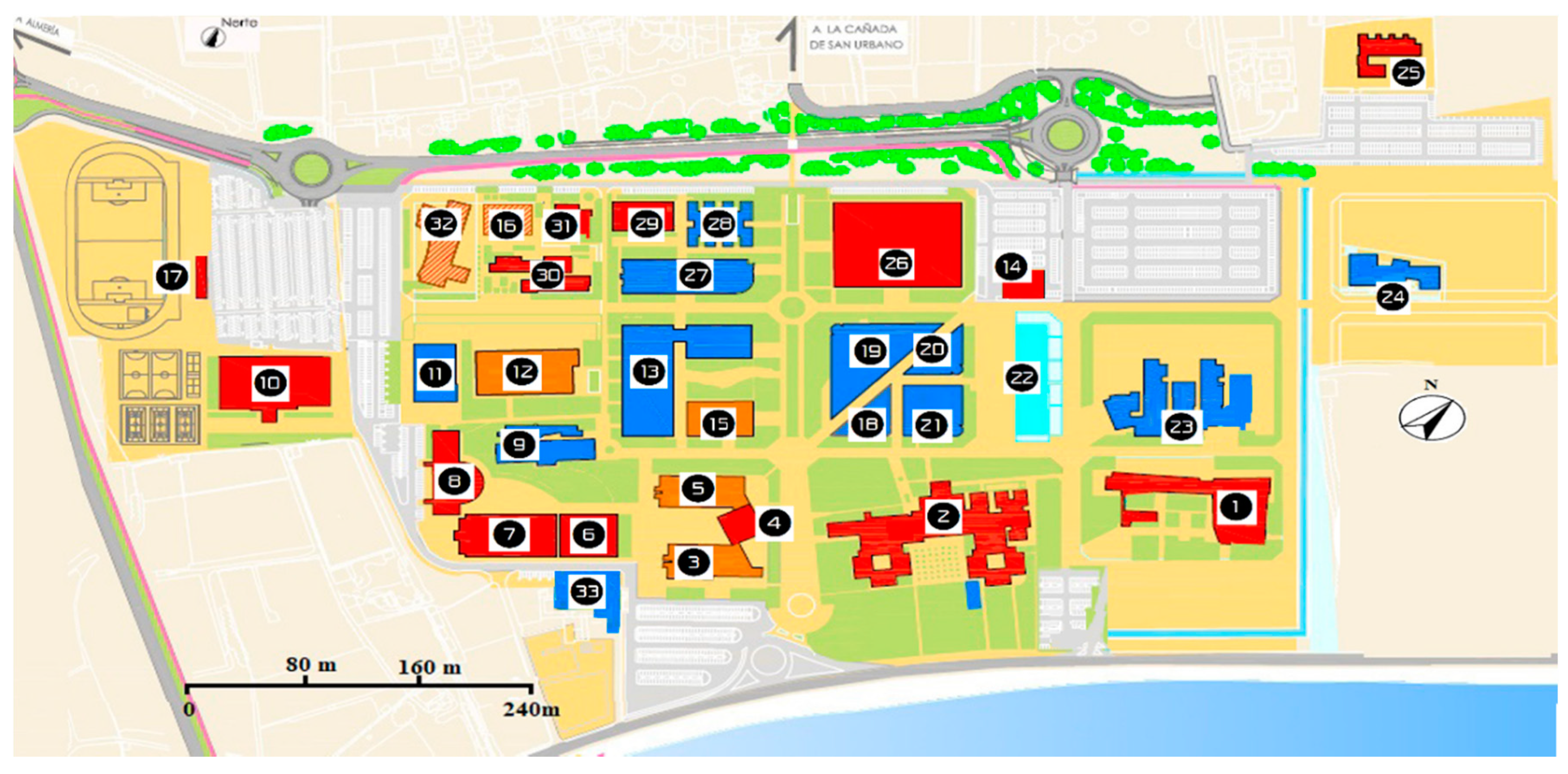
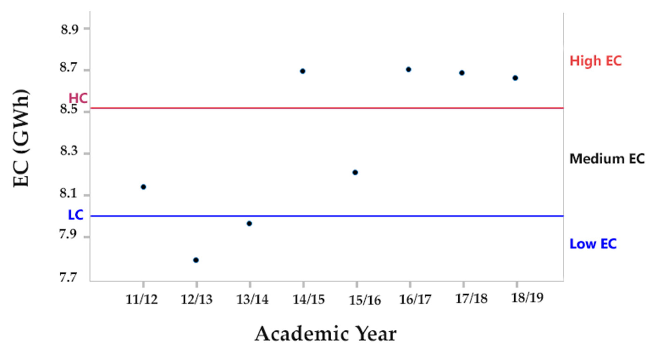
Table 3 contains values of the electricity performance metrics of all the categories in the campus, and they are cited in Table 3 from the highest to lowest intensity. Average EUIs were calculated by first calculating the average in the three years of each building. Then, we sum up the EUIs within the category, and we dived them by the number of facilities of each category. The section of others is excluded from the benchmark study because it includes three buildings (14,22,25) that represent, respectively, a warehouse, a parking garage, and a nursery. These buildings have a weak EC, do not have an impact on the campus EC, and do not fit into any of the major categories. The EUI averages represent benchmark values of the cited categories in the Mediterranean climate.

Figure 3 and Figure 4 summarize as percentages the total EC by categories and the sum total GFA by categories. The research and science category have the biggest share by 47% of the EC, even though it accounts for only 27% of the gross floor area (GFA), followed by the teaching and seminary category that accounts 17% of the EC and 26% of the GFA, the library category that accounts 15% of the EC and 7% of the GFA, the administration office category that accounts 15% of the EC and 27% of the GFA, by the sport facilities category that account 5% of the EC and 6% of the GFA, and finally the restaurant category that accounts 1% and 2% of the GFA. These distribution shows that there is no direct relation relationship between EC and GFA because each category has its own characteristics.

Figure 5 summarizes the energy consumption evolution by building category from 2016 to 2018. The evolution of the total sum campus EC had a minimum value in 2016, then had peaked in 2017, and had medium value in 2018. Figure 5 reveals that all the categories followed the overall trend, except restaurant and sport facilities, where both categories account combined 6% of the total EC. Research building EUI varies from 32.5–230.3 kWh/m². Furthermore, its facilities include spaces like academic offices, computer rooms, and laboratories, and those spaces are characterized by a longer period of operation and a large number of computers, laboratory freezers, and other electric equipment. However, the majority of research buildings have a value superior to 80 kWh/m²; the highest intensity value—230.3 kWh/ m²—was scored by the solar energy center building (31). One of the reasons behind this high consumption is that a lot of research takes place in the center, and the researchers and students working on solar chemistry and water detoxification use several compressors with high energy consumption that cannot be powered small solar field installed on the roof of the building. The technology of information and communication center building (30) has the second highest value 188.3 kWh/m², and the lowest value was scored by the engineering school building (9).

Library building EUI varies from 62.4–105.3 kWh/m². This category is the second most energy intensive. Their locals include spaces like reading rooms, computer rooms, and common spaces and are characterized by a centralized air conditioning system, longer operating time, a high number of occupants (especially during the exam period), and a substantial number of computers and laptops.

Sport facilities are the third biggest consumer of energy by GFA, and their EUI varies from 28.02–69.9 kWh/m². It contains spaces like swimming pool, a covered multitask hall, and gym rooms.

Restaurant buildings had the fourth highest energy intensity, and their EUI varies from 35.13–41.34 kWh/m². They are characterized by longer operating time and different electric equipment.

Teaching and seminary rooms had the fifth highest energy intensity, and their EUI varies from 13.59–59.2 kWh/m². This category includes spaces like regular classrooms, computer rooms, and room theaters, and it is characterized by a high number of occupants. Four buildings out of eight have similar EUI values, which are close to average energy use index of this category. The lowest value is scored by building (4), a seminary building that has a low operating frequency, while the highest value is scored by building (3), which is an exception in this category because of its infrastructure that includes a water pumping system to get rid of the used water for the whole campus.

Administration offices are the least energy intensive category, and their EUI varies from 23.3–32.5 kWh/m². They include offices, meeting rooms, and common spaces and are characterized by a low number of occupant and shorter operating time.

Figure 6 outlines the scatter plot of the average EUI during last three years. In the function of the average EC, we can observe that only five buildings (31,30,29,24,32) have an EUI superior to the EUI median of universities (MU) in the Mediterranean climate given by the 2003 CBECS data [9]. Twenty-five buildings from our portfolio have an energy intensity inferior than the M.U, and 19 out of those 25 buildings are three time less intense than the k–12 schools in hot and humid zones [9]. In addition, the scatter plot demonstrates that four buildings (30,29,13,26) have an EC greater than 7.0 × 10⁵ kWh. These facilities belong to the research and library category. However, two of those big consumers have EUI values bellow the MU, and the category that has shown more harmony in their sample of buildings is the restaurant category, which include two properties that has almost identical values in their EC, GFA, and EUI.

Table 4 outlines the classification of energy performance of all the buildings within each category. This classification is a useful tool for managers because it reports insights into which of the building should be prioritized in term of investments to achieve efficiency. Managers an divide the portfolio of every category into three groups (poor practice, usual practice, and best practice).

3.2. Case Study

Figure 7 summarizes the campus yearly energy consumption from 2011 to 2018. The overall energy consumption has been varying in the range of 7.93–8.8 GWh, and it has a known growth of 9% since 2011. However, the patterns do not represent a clear trend through the calendar years; this is one of the reasons we decided to proceed with the academic years since we have the data of the campus monthly EC (Table 1).

Campus energy consumption data on a monthly basis (Table 1) shows that the evolution over the years is generally the same, which means that it plunges and peaks in the same period of the year. The peaks usually happen during the months of May and June. In this period, campus buildings make substantial use of HVAC systems, and some buildings like the library start operating for a longer period because of the exam period. The down trend starts in October after the weather begins to be cooler, and in the beginning of July, it plunges to hit the lowest values in August—during this period, the campus is practically empty, and the majority of the university buildings are non-operational because of the summer vacation.

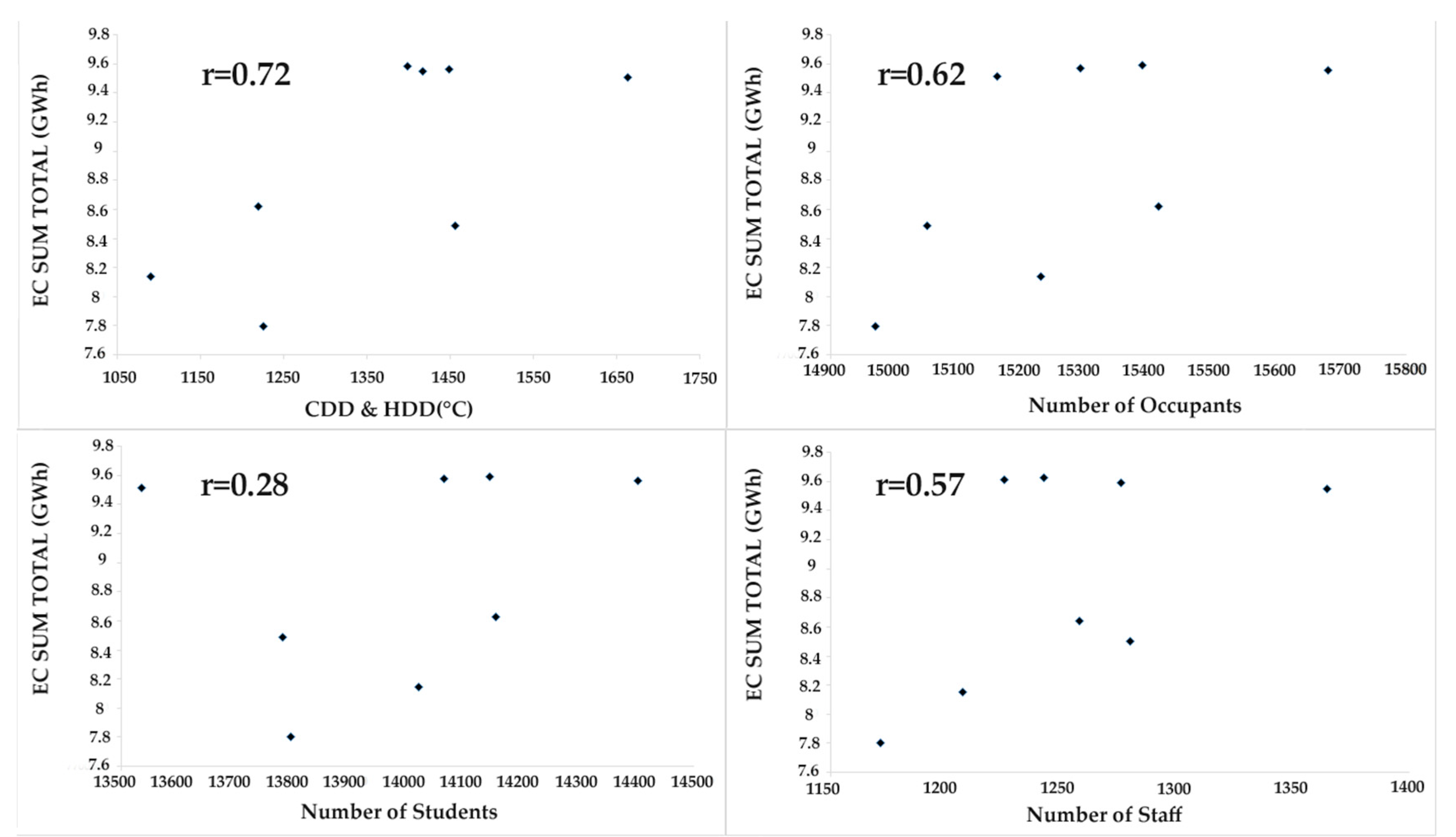
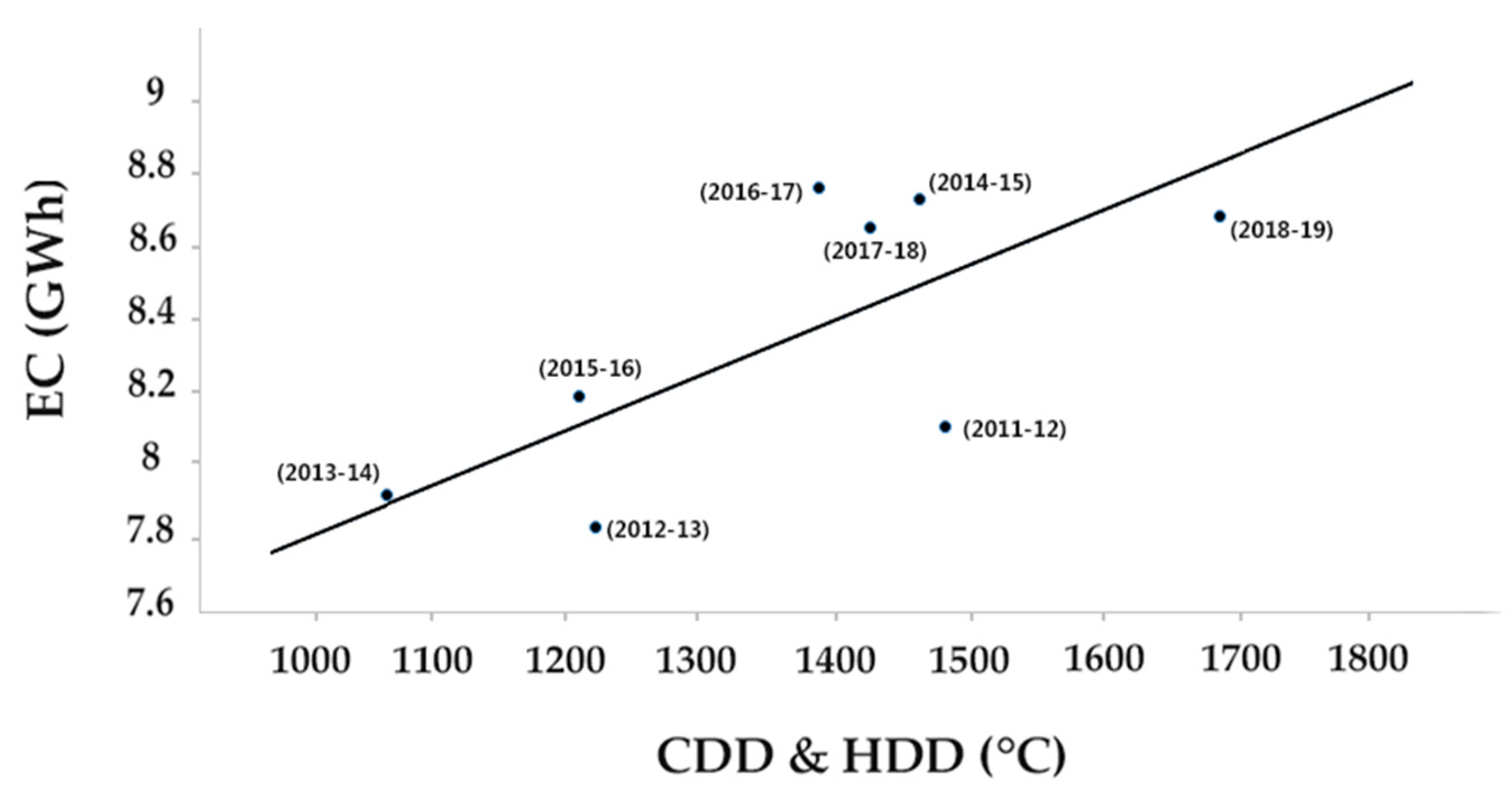
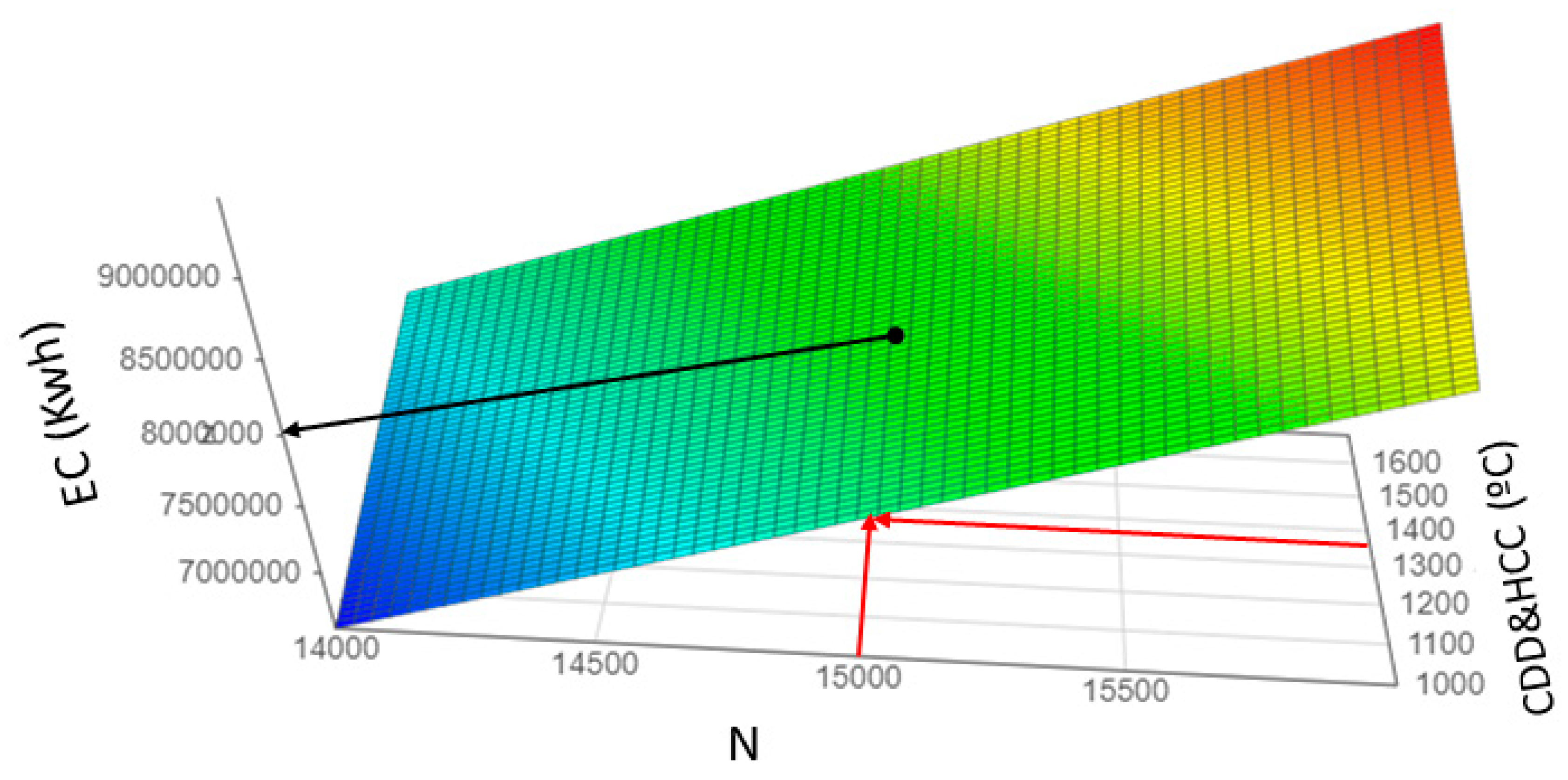
3.3. Correlation Analysis and Regression Model

Data presented in Table 5 sums up the inputs and the outputs used for the correlation analysis and regression model which corresponds to weather parameters (CDD and HDD), the number of occupants (the number of students, professors, and administration staff), and the EC of the campus.

Figure 8 outlines the scatter plots of EC sum total of the campus in function of the following variables: CDD and HDD, number of occupants, number of students, and number of staff. In the case of the correlation of outdoor temperature with EC, EC (Kwh) = 1204.8 CDD&HCC (°C) + 7·10 ⁶, its correlation coefficient of 0.72 indicates a positive correlation. According to the scatter plot of the number of occupants, its correlation coefficient of 0.62, which also indicates a positive correlation (EC (Kwh) = 1073.9.7 N—8·10 ⁶). However, the remaining scatter plots represented a weak correlation, especially for the number of students. In addition, the number of occupants is the main factor behind the excessive consumption.

Figure 9 outlines the linear regression model of the total EC as a function of CDD and HDD. Both variables are statistically related because the correlation coefficient is 0.719. Figure 10 shows the energy thresholds of good practice of the University of Almeria.

$$Lc=\frac{\mathrm{Min}1\left(\mathrm{EC}\right)1+\mathrm{Min}2\left(\mathrm{EC}\right)+\mathrm{Min}3\left(\mathrm{EC}\right)}{3}$$

$$Hc=\frac{\mathrm{Med}1\left(\mathrm{EC}\right)1+\mathrm{Med}2\left(\mathrm{EC}\right)+\mathrm{Med}3\left(\mathrm{EC}\right)}{3}$$

4. Discussion

4.1. Benchmark Analysis

Dividing campus facilities into categories allows us to compare buildings based on their utility and to identify the category that has the lowest and largest energy consumption by GFA. The category that scored the highest EUI average in this case study is the research and science category by an average metric score of 119.5 kWh/m², which is inferior to the laboratory intensity median given by CBECS 2003 data by Oak Ridge National Lab and the Department of Energy, which is 226 kWh/m² for the Mediterranean climate [9]. In another comparative study, which was conducted at the regional scale in the state of California (Mediterranean climate), they showed that some laboratories scored the highest energy intensity with a value of 909.5 kWh/m², and it is four times bigger than the state average energy intensity [29,30,31]. The results in our study have proven that this category can provide a wide range of energy intensity, which makes it worthy of more in-depth study. The observations indicate that the longer operation hours inside the facilities of the research and science category, its heavy plug load materials (like ultra-low freezers and incubators), and other laboratory equipment are the reason behind the high intensity. In addition, the high number of computers used are the reason behind the high intensity. The second most intense category is the library category, which accounts for only 7% of the total GFA but contributes to 15% in of total EC. The buildings in this category peak during the months of the preparation of exams, especially in the summer session, when their EC becomes three times higher, unlike the teaching and seminary rooms, which have a slight increase during the same period when the teaching days are relatively lower. Our portfolio have an EUI inferior than 50 kWh/m² (Figure 6), which is the equivalent of one third of the k–12 schools in hot and humid zones. This brings back the question of which is more energy intense—schools or universities—and how much can the weather parameter contribute to the increase of electricity consumption. Thus, there are several parameters other than the weather to take into consideration, such as occupancy rate, number of COM, plug load, and operating time, that are responsible for the EC gap between different categories. On the other hand, simulation techniques represent one of the efficient alternatives to evaluate the energy performance of a building regardless of its utility. This method was used to develop a benchmark analysis based on models of equipment and system performance, which proved that plug loads and HVAC are some of the biggest influencers of high energy consumption in laboratory buildings.

4.2. Correlation Analysis

Despite the complexity of EC in university campuses, we were able to demonstrate that outdoor temperature and number of occupants positively correlate with the overall energy use, which confirmed our choice of variables. Nevertheless, another study that developed a simulation of the building occupants’ decision-making and information communication process found that the network size has no significant impact on the EC [32]. Still, that result needs to be confirmed in non-residential building, especially in cases like schools and universities, where the number of occupants changes substantially over the year. On the other hand, a study that was conducted on 10 universities in the US and confirmed that EC correlates highly with outdoor temperature [33]. Weather variations can easily change cooling and heating use by 20–30% [34]. The estimation of the occupancy rate for each building remains challenging, especially in this case study because of the irregular patterns of the student movement inside the campus, which is not only related to the classes or other scheduled activities. Nonetheless, some studies used CO₂ measuring, relative humidity, and acoustic sensors to estimate occupancy [35,36,37]; however, those techniques are hard to implement in our case of study because of the several components that the buildings incorporate. On the other hand, many studies [38,39] have focused on the behavior of occupants rather than the size of active occupants. In order to evaluate the energy saving potential, one study developed an occupancy model of individuals moving in and out in offices [40], while another study found an alternative to analyze occupancy patterns using physical-statistical approaches to improve energy demand forecasting [35,41]. Still, identifying how occupant’s behavior influences EC is complex because of the stochastic nature of individual actions [37].

The five buildings (31,30,29,24,32) from our portfolio scored a higher energy intensity than the university in a Mediterranean climate median. Installing solar panels on the roof as a backup is highly recommended since the campus is located on southern coast of Spain, where the yearly sum of global irradiation is over 1900 kWh/m² [41]. Therefore, efforts and investments have to prioritize these facilities because they are driving the high consumptions and there is a considerable gain potential to achieve from their high energy intensity.

If a model with the two explicative variables (N and CDD&HCC) is established and a multiple regression is conducted, Equation (4) is obtained.

$$\mathrm{EC}\left(\mathrm{Kwh}\right)=1050.375608\mathrm{N}+1172.322578\mathrm{CDD}\&\mathrm{HCC}\left(°\mathrm{C}\right)-9320518.243$$

(4)

with R² = 0.83. If the model obtained is plotted (see Figure 11), the range of expected energy consumption can be found according to the parameters of number of occupants (N) and CDD and HCC in °C. Therefore, a threshold of 8 GWh has been estimated as the energy consumption limit to be achieved for 15,000 persons and for a CDD and HCC of 1350 °C, both factors being the average of the last eight years.

5. Conclusions

Gathering high resolution outdoor temperature data during the last eight years with half an hour time frame was important for this case of study because it provided the opportunity to calculate cooling and heating degree-days. The weather factor is the most significant variable in this case study, which means that the university administration will achieve better results in term of reducing end user costs by investing in the efficiency of the HVAC system and then improving the thermal performance of the campus buildings. It has been found that research buildings consume four times more energy than teaching or administration buildings. In addition, behavioral changing programs are recommended, especially in cases like ours, where the properties are open to the public and the managers are challenged to lead the users toward sustainable actions—for instance, starting a program that aims to share information about the evolution and the gains of EC with the students and staff which could be useful to raise awareness about the continuous increase of energy use inside the campus. A similar experiment was executed in dormitory residences, and the results show that the group of residents who received real-time data feedback were more effective in energy conservation gains. The buildings from our portfolio that scored a higher energy intensity should consider installing solar panels on their roofs. Additionally, setting up systems like occupancy sensors for automatic lighting will increase efficiency. Nonetheless, energy conservation measures should not affect the indoor quality; for this reason, we must be able to reduce EC while retaining indoor quality.

References

1. Pino-Mejías, R.; Pérez-Fargallo, A.; Rubio-Bellido, C.; Pulido-Arcas, J.A. Artificial neural networks and linear regression prediction models for social housing allocation: Fuel Poverty Potential Risk Index. Energy 2018, 164, 627–641. [Google Scholar] [CrossRef]
2. Forcael, E.; Nope, A.; García-Alvarado, R.; Bobadilla, A.; Rubio-Bellido, C. Architectural and Management Strategies for the Design, Construction and Operation of Energy Efficient and Intelligent Primary Care Centers in Chile. Sustainability 2019, 11, 464. [Google Scholar] [CrossRef] [Green Version]
3. Bienvenido-Huertas, D.; Rubio-Bellido, C.; Pérez-Ordóñez, J.L.; Martínez-Abella, F. Estimating adaptive setpoint temperatures using weather stations. Energies 2019, 12, 1197. [Google Scholar] [CrossRef] [Green Version]
4. Sánchez-García, D.; Rubio-Bellido, C.; Tristancho, M.; Marrero, M. A comparative study on energy demand through the adaptive thermal comfort approach considering climate change in office buildings of Spain. Build. Simul. 2020, 13, 51–63. [Google Scholar] [CrossRef]
5. Wright, T.S.; Wilton, H. Facilities management directors’ conceptualizations of sustainability in higher education. J. Clean. Prod. 2012, 31, 118–125. [Google Scholar] [CrossRef]
6. Hodgson, M.; Brodt, W.; Henderson, D.; Loftness, V.; Rosenfeld, A.; Woods, J.; Wright, R. Needs and opportunities for improving the health, safety, and productivity of medical research facilities. Environ. Health Perspect. 2000, 108 (Suppl. 6), 1003–1008. [Google Scholar] [CrossRef] [Green Version]
7. Rastegar, M.; Fotuhi-Firuzabad, M.; Zareipour, H. Home energy management incorporating operational priority of appliances. Int. J. Electr. Power Energy Syst. 2016, 74, 286–292. [Google Scholar] [CrossRef]
8. ANSI/ASHRAE/IES Standard 100-2015, Energy Efficiency in Existing Buildings; ANSI/IES/ASHRAE: Atlanta, GA, USA, 2015.
9. ANSI/ASHRAE/IES Standard 55-2015, Developing Energy performance Targets for ASHRAE Standard; ANSI/IES/ASHRAE: Oak Ridge, TN, USA, 2015.
10. The Energy Efficiency Directive. (2012/27/EU). Available online: https://ec.europe.eu/energy (accessed on 22 December 2019).
11. Krarti, M. Energy Audit of Building Systems: An Engineering Approach; CRC Press: Boca Raton, FL, USA, 2016. [Google Scholar]
12. Lara, R.A.; Pernigotto, G.; Cappelletti, F.; Romagnoni, P.; Gasparella, A. Energy audit of schools by means of cluster analysis. Energy Build. 2015, 95, 160–171. [Google Scholar] [CrossRef]
13. AlFaris, F.; Juaidi, A.; Manzano-Agugliaro, F. Improvement of efficiency through an energy management program as a sustainable practice in schools. J. Clean. Prod. 2016, 135, 794–805. [Google Scholar] [CrossRef]
14. Henderson, K.; Tilbury, D. Whole School Approaches to Sustainability: An International Review of Sustainable School Programs; Macquarie University: Sydney, NSW, Australia, 2004. [Google Scholar]
15. Serrano-Guerrero, X.; Escrivá-Escrivá, G.; Roldán-Blay, C. Statistical methodology to assess changes in the electrical consumption profile of buildings. Energy Build. 2018, 164, 99–108. [Google Scholar] [CrossRef]
16. Roldán-Blay, C.; Escrivá-Escrivá, G.; Roldán-Porta, C. Improving the benefits of demand response participation in facilities with distributed energy resources. Energy 2019, 169, 710–718. [Google Scholar] [CrossRef]
17. Escrivá-Escrivá, G.; Roldán-Blay, C.; Roldán-Porta, C.; Serrano-Guerrero, X. Occasional Energy Reviews from an External Expert Help to Reduce Building Energy Consumption at a Reduced Cost. Energies 2019, 12, 2929. [Google Scholar] [CrossRef] [Green Version]
18. Wang, K.; Wang, Y.; Sun, Y.; Guo, S.; Wu, J. Green industrial Internet of Things architecture: An energy-efficient perspective. IEEE Commun. Mag. 2016, 54, 48–54. [Google Scholar] [CrossRef]
19. Mathew, P.A.; Dunn, L.N.; Sohn, M.D.; Mercado, A.; Custudio, C.; Walter, T. Big-data for building energy performance: Lessons from assembling a very large national database of building energy use. Appl. Energy 2015, 140, 85–93. [Google Scholar] [CrossRef] [Green Version]
20. Khoshbakht, M.; Gou, Z.; Dupre, K. Energy use characteristics and benchmarking for higher education buildings. Energy Build. 2018, 164, 61–76. [Google Scholar] [CrossRef] [Green Version]
21. Mills, E.; Bell, G.; Sartor, D.; Chen, A.; Avery, D.; Siminovitch, M.; Greenberg, S.; Marton, G.; de Almeida, A.; Lock, L.E. Energy Efficiency in California Laboratory-Type Facilities; LBNL Report #39061; Ernest Orlando Lawrence Berkeley National Laboratory: Berkeley, CA, USA, 1996; Available online: https://www.aivc.org/sites/default/files/airbase_11236.pdf (accessed on 20 December 2019).
22. Chen, Y.-T. The Factors Affecting Electricity Consumption and the Consumption Characteristics in the Residential Sector—A Case Example of Taiwan. Sustainability 2017, 9, 1484. [Google Scholar] [CrossRef] [Green Version]
23. Pickering, C.; Byrne, J. The benefits of publishing systematic quantitative literature reviews for PhD candidates and other early-career researchers. High. Educ. Res. Dev. 2014, 33, 534–548. [Google Scholar] [CrossRef] [Green Version]
24. Aemet. Spanish State Meteorological Agency (Agencia Estatal de Meteorología en España). Available online: http://www.aemet.es/ (accessed on 20 December 2019).
25. Manzano-Agugliaro, F.; Montoya, F.G.; Sabio-Ortega, A.; García-Cruz, A. Review of bioclimatic architecture strategies for achieving thermal comfort. Renew. Sustain. Energy Rev. 2015, 49, 736–755. [Google Scholar] [CrossRef]
26. Kipping, A.; Trømborg, E. Modeling aggregate hourly energy consumption in a regional building stock. Energies 2017, 11, 78. [Google Scholar] [CrossRef] [Green Version]
27. Cheng, V.; Steemers, K. Modelling domestic energy consumption at district scale: A tool to support national and local energy policies. Environ. Model. Softw. 2011, 26, 1186–1198. [Google Scholar] [CrossRef]
28. Fumo, N.; Biswas, M.R. Regression analysis for prediction of residential energy consumption. Renew. Sustain. Energy Rev. 2015, 47, 332–343. [Google Scholar] [CrossRef]
29. Huizenga, C.; Liere, W.; Bauman, F.; Arens, E. Development of Low-Cost Monitoring Protocols for Evaluating Energy Use in Laboratory Buildings; Center for Environmental Design Research; University of California: Berkeley, CA, USA, 1996. [Google Scholar]
30. Federspiel, C.; Zhang, Q.; Arens, E. Model-based benchmarking with application to laboratory buildings. Energy Build. 2002, 34, 203–214. [Google Scholar] [CrossRef] [Green Version]
31. Chen, J.; Taylor, J.E.; Wei, H.H. Modeling building occupant network energy consumption decision-making: The interplay between network structure and conservation. Energy Build. 2012, 47, 515–524. [Google Scholar] [CrossRef]
32. Jafary, M.; Wright, M.; Shephard, L.; Gomez, J.; Nair, R.U. Understanding Campus Energy Consumption--People, Buildings and Technology. In Proceedings of the 2016 IEEE Green Technologies Conference (GreenTech), Kansas City, MO, USA, 6–8 April 2016; pp. 68–72. [Google Scholar]
33. Cox, R.A.; Drews, M.; Rode, C.; Nielsen, S.B. Simple future weather files for estimating heating and cooling demand. Build. Environ. 2015, 83, 104–114. [Google Scholar] [CrossRef] [Green Version]
34. Erickson, V.L.; Carreira-Perpiñán, M.Á.; Cerpa, A.E. OBSERVE: Occupancy-based system for efficient reduction of HVAC energy. In Proceedings of the 10th ACM/IEEE International Conference on information processing in sensor networks, Chicago, IL, USA, 12–14 April 2011; pp. 258–269. [Google Scholar]
35. Khan, A.; Nicholson, J.; Mellor, S.; Jackson, D.; Ladha, K.; Ladha, C. Occupancy monitoring using environmental & context sensors and a hierarchical analysis framework. In Proceedings of the BuildSys 2014: 1st ACM International Conference on Embedded Systems for Energy-Efficient Buildings, Memphis, TN, USA, 4–6 November 2014; pp. 90–99. [Google Scholar] [CrossRef]
36. Chen, J.; Ahn, C. Assessing occupants’ energy load variation through existing wireless network infrastructure in commercial and educational buildings. Energy Build. 2014, 82, 540–549. [Google Scholar] [CrossRef]
37. Masoso, O.T.; Grobler, L.J. The dark side of occupants’ behaviour on building energy use. Energy Build. 2010, 42, 173–177. [Google Scholar] [CrossRef]
38. Pilkington, B.; Roach, R.; Perkins, J. Relative benefits of technology and occupant behaviour in moving towards a more energy efficient, sustainable housing paradigm. Energy Policy 2011, 39, 4962–4970. [Google Scholar] [CrossRef]
39. Chang, W.K.; Hong, T. Statistical analysis and modeling of occupancy patterns in open-plan offices using measured lighting-switch data. Build. Simul. 2013, 6, 23–32. [Google Scholar] [CrossRef] [Green Version]
40. Lü, X.; Lu, T.; Kibert, C.J.; Viljanen, M. Modeling and forecasting energy consumption for heterogeneous buildings using a physical–statistical approach. Appl. Energy 2015, 144, 261–275. [Google Scholar] [CrossRef]
41. Montoya, F.G.; Aguilera, M.J.; Manzano-Agugliaro, F. Renewable energy production in Spain: A review. Renewable and Sustainable Energy Reviews, 33, 509–531. Renew. Sustain. Energy Rev. 2014, 33, 509–531. [Google Scholar] [CrossRef]
Figure 1. The University of Almeria ground plan.
Sustainability 12 01336 g001
Figure 2. Methodology top-down chart.
Sustainability 12 01336 g002
Figure 3. Energy consumption (EC) proportion of all the categories.
Sustainability 12 01336 g003
Figure 4. Gross floor area (GFA) proportion of all the categories.
Sustainability 12 01336 g004
Figure 5. Energy consumption evolution by building category.
Sustainability 12 01336 g005
Figure 6. Scatter plot of energy use intensity (EUI) as a function of energy consumption (EC) by buildings category.
Sustainability 12 01336 g006
Figure 7. Campus yearly consumption 2011–2018.
Sustainability 12 01336 g007
Figure 8. Scatter plots with their correspondent coefficient of correlation.
Sustainability 12 01336 g008
Figure 9. Linear regression model of EC in function of CDD and HDD.
Sustainability 12 01336 g009
Figure 10. Scatter plot of the total EC in function of academic year
Sustainability 12 01336 g010
Figure 11. Energy consumption (EC) model obtained for the explicative variables: N (number of occupants) and CDD and HCC (°C).
Sustainability 12 01336 g011