Article

Validation of Simulated Safety Indicators with Traffic Crash Data

1
Department of Transport and Project and Process Technology, University of Cantabria, Avda. De Los Castros, 44, 39005 Santander, Spain
2
Department of Civil Engineering, University of Calabria, 87036 Arcavacata, Italy
*
Author to whom correspondence should be addressed.
Sustainability 2020, 12(3), 925; https://doi.org/10.3390/su12030925
Submission received: 31 December 2019 / Revised: 17 January 2020 / Accepted: 20 January 2020 / Published: 27 January 2020

Abstract

:
The purpose of this document is to validate a new methodology useful for the estimation of road accidents resulting from possible driver distractions. This was possible through a statistical comparison made between real accident data between 2016 and 2018 in the city of Santander (Spain) and simulated data resulting from the application of the methodology on two areas of study. The methodology allows us to evaluate possible collisions starting from the knowledge of vehicular trajectories extrapolated from microsimulation. Studies show that there are good correlations between the real data and the simulated data. The results obtained show that the proposed methodology can be considered reliable and, therefore, it could be of fundamental importance for designers, since it would simplify the choice between different possible intervention scenarios, determining which is the least risky in terms of road safety.

1. Introduction

The main methodology for the identification of dangerous locations, commonly named black spots, relies on the use of crash databases [1,2,3,4,5,6,7,8]. Statistical and analytical methodologies applied to crash databases allow us to establish a connection between the causes (roads) and effects (accidents) and allow the extraction of useful information for road safety improvement. These procedures, unfortunately, cannot be used to perform better planning of new roads or to perform a detailed evaluation of possible modifications of the road infrastructure. Moreover, the physical process, which would explain the relationship between causes and effects, is not established and stays hidden behind the statistical modelling.
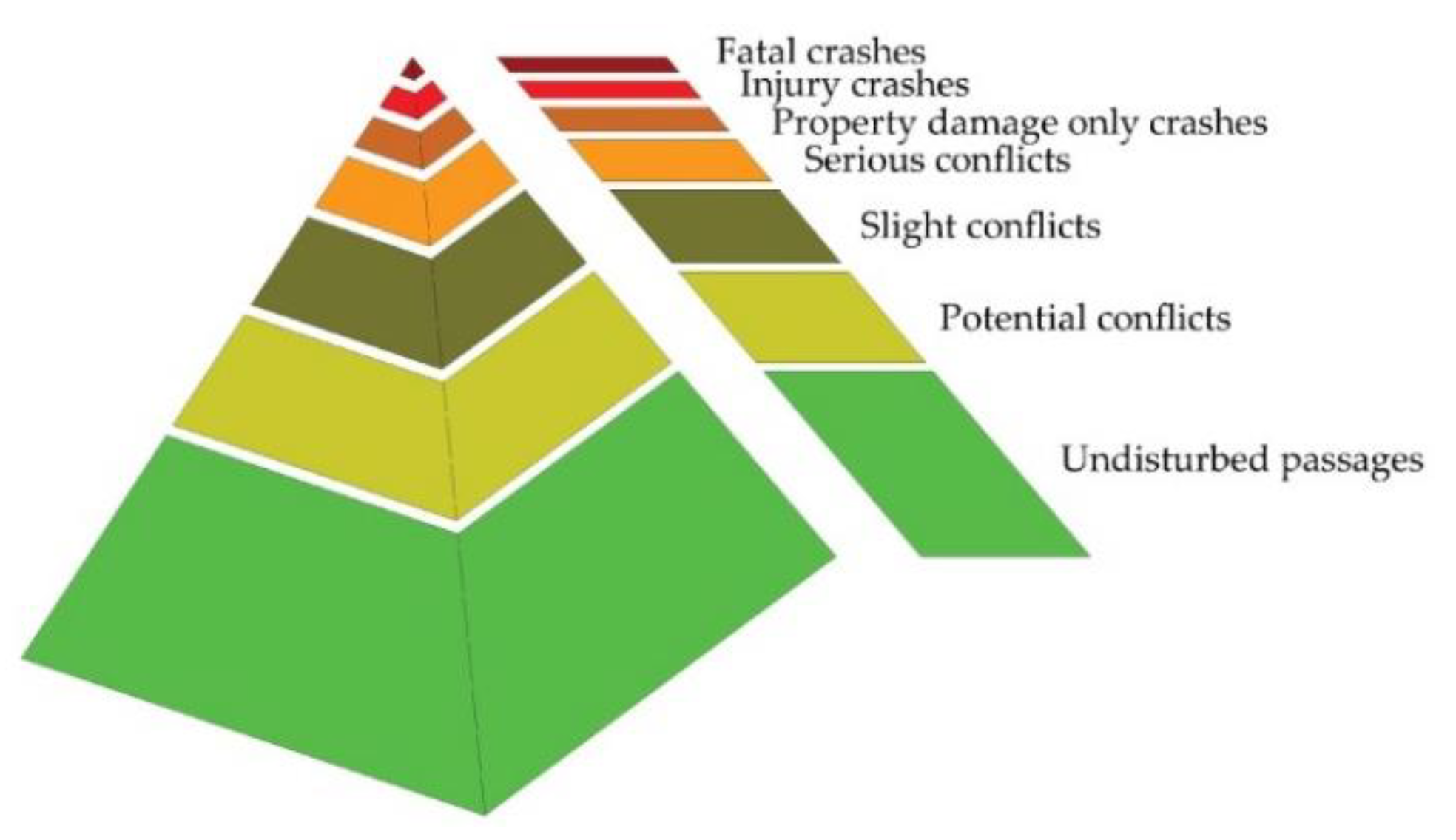
For these reasons, an alternative procedure was developed at the end of the 1960s. The concept is that of using traffic conflict data instead of crash data. Traffic conflicts are events in which crashes are more likely since drivers are driving close to each other. In 1987, Hydén [9] developed the concept of a “safety pyramid, or Hydén pyramid” (Figure 1) thanks to which it is possible to take into account all the possible interaction events that are inevitably created within any vehicular flow. According to this research, there is a connection between the severity of the event and the probability that it will occur. According to this approach, the most probable events are less serious ones, while less probable events are the most serious.
The prerequisite to applying this kind of procedure is that of using vehicle trajectories to assess safety levels by evaluating the number or the severity of dangerous situations that can occur on certain road infrastructure. All the studies carried out on this subject are based on the identification of so-called “surrogate safety indicators”, which seek to evaluate the potentially dangerous interactions between vehicles and to determine which of these may lead to dangerous—or, in any case, anomalous—events.
Among these surrogate safety indicators, the best known are Time to Collision (TTC) and Post-Encroachment Time (PET). In 1971, Hayward [10] introduced the use of TTC (Figure 2), which is the time in which two vehicles would collide if they continued travelling on the same trajectory with their speeds unchanged.
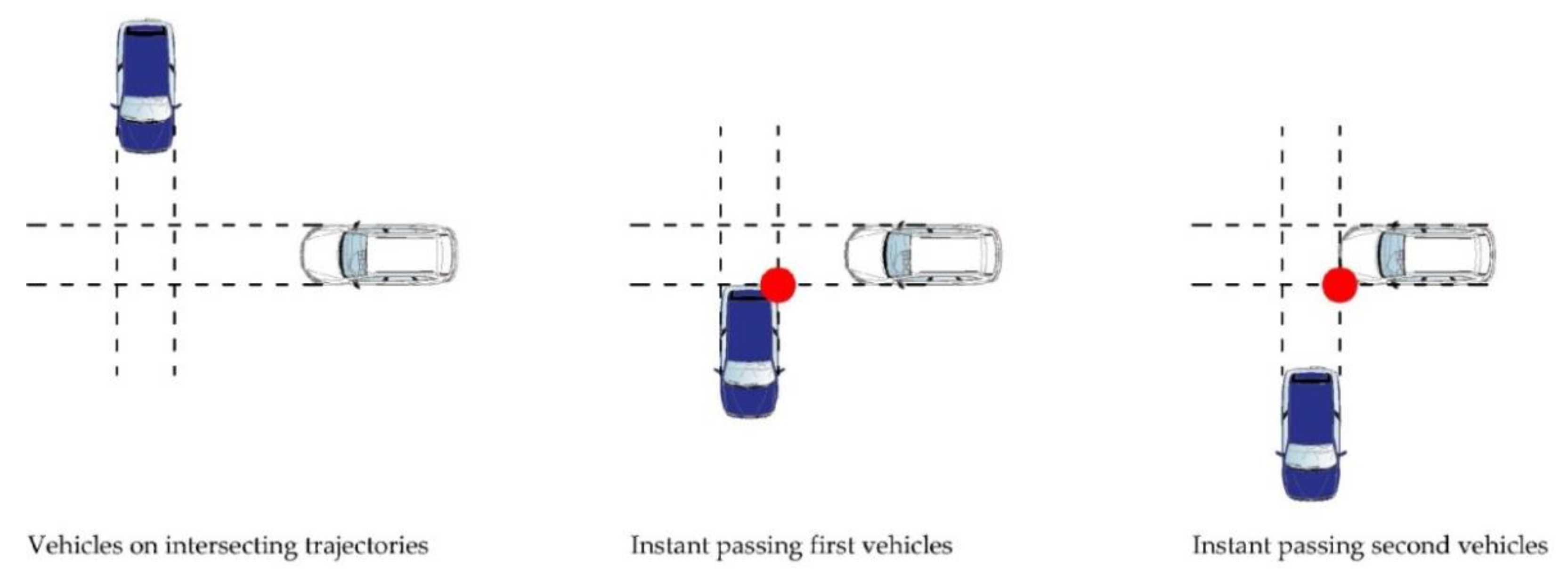
The PET time (Figure 3) was applied for the first time in the field of road safety assessment in 1978 by Allen et al. [11]. Considering vehicles on intersecting trajectories, the PET time is calculated from the moment in which the first vehicle passes at the intersection point until the moment when the second vehicle also passes.
The first implementations of surrogate safety indicators were applied to real trajectories (especially at intersections). Trajectories can also be generated by microsimulation. With the idea of evaluating traffic safety levels in a microsimulation environment, the Software Surrogate Safety Assessment Model (SSAM) [12] was developed in 2008. SSAM is able to identify, classify and evaluate the various conflicts that can be generated between different vehicles in a network in an automatic way (generally, the Software considers the possibility of a conflict occurring in the event that TTC ≤ 1.5 s or PET ≤ 5 s). SSAM analyses the trajectories extracted from some of the most well-known microsimulation software—including AIMSUN [13], VISSIM [14], Paramics [15] and TEXAS [16]—and identifies and catalogs every possible conflict. In addition, for each conflict, SSAM establishes the values of TTC, PET, etc.
Recently, three meticulously compiled papers present a state of the art on traffic conflicts, road safety simulation modelling and on the use of surrogate safety measures [17,18,19]. All these three works indicate some of the limitations of using microsimulation and surrogate safety measures.
Young et al. [18] recognize the potential for simulation to become a useful tool for road traffic safety, yet they also state that further research is needed since driver behaviours that may generate an accident have not been considered holistically in simulation. Moreover, they affirm that “The theory behind driver behaviour in crashes” and the presence of heavy vehicles are not commonly taken into account.
Zheng et al. [19] point out that common traffic safety indicators consider only the occurrence of conflicts without taking into consideration the real consequences of a potential crash: “proximity measure can only reflect the risk of collision but not the severity of crashes, which is typically differentiated based on consequences of the crash, not proximity.”
Furthermore, Laureshyn et al. [20] explain that commonly used surrogate safety performance measures convey “proximity” to a crash and overlook the potential severity of the consequences of a crash. The consequences need to be taken into account in some way [21].
Crash severity is an extremely important measure [22] and, strangely, the severity of potential crashes was only introduced in surrogate safety indicators in 2017, with the Extended Delta-V method [20]. Delta-V commonly means the variation of the speed vector V of a vehicle after an accident. This value can describe the magnitude of the impact, taking into consideration vehicle dynamics and physical dimensions; in fact, if you consider, for example, the impact between a very small vehicle with one of large dimension, it will occur that the first vehicle will bounce while the second will continue its motion almost unaffected.
Moreover, the elephant in the room for the current application of these methodologies lies in the important, easily observable fact that not all accidents are caused by vehicles travelling on conflicting trajectories. According to statistics, collisions between isolated vehicles and fixed objects are extremely important in road safety [23,24,25], and account of more than 40% of all fatal accidents (not involving pedestrians or bicycles).
In other words, all previously introduced road traffic safety indicators are incomplete in their use since they are based on conflict techniques that do not take into account roadside obstacles and barriers.
Traditionally in transportation engineering, quantitative approaches have been applied to solve congestion problems with attempts to shift demand on transit systems [26] and to implement better road traffic control by adopting tools such as traffic simulation [18,27,28,29,30,31] dynamic network loading equilibrium, dynamic models [32,33,34,35] and methodologies attempting to affect user route choice [36,37,38,39,40]. Quantitative approaches involving network modelling have seldom been applied to Traffic Safety evaluation.
The above-indicated limitations are possibly among the reasons why simulation was never used to find out black spots and to evaluate safety levels in current engineering practices.
To address these problems and to boost the use of microsimulation for the assessment of traffic safety levels in 2018, in the Department of Civil Engineering of the University of Calabria, the Zombie Driver (ZD) methodology was developed [29]. The methodology follows the traditional approach of conflict based indicators and can be applied to real vehicular trajectories or simulated trajectories derived from microsimulation environments such as AIMSUN [13], VISSIM [14] and Tritone [28,41]. This methodology can encompass all the aspects described, and also introduces the human factor (the possible distraction of the users) as a trigger for accident events.
The objective of this document will, therefore, be the validation of the latter methodology and, a comparison with other previously introduced surrogate safety indicators. Results of the analysis carried out show a better correlation between the newly proposed indicator and real crash data than other more commonly used classic indicators.

2. Materials and Methods

2.1. A New Surrogate Safety Indicator: from Traffic Conflict Simulation to Traffic Crash Simulation

The Zombie Driver methodology [29] can only be applied following the acquisition of vehicular trajectories. In this work, the Tritone Software [28,41] was used for the extrapolation of vehicular trajectories. Tritone is a complete microsimulation environment that can simulate traffic in a network instant-by-instant, based on road geometry and the behaviour of drivers, considering also specific vehicle characteristics.

2.1.1. Tritone Simulation Model Can Produce Trajectories and Traditional Safety Performances Indicators Such as TTC and PET Using the Same Algorithms of SSAM

To do this, a series of models were implemented in Tritone with which it was possible to describe the behaviour of every vehicle introduced into the network for every instant of simulation. Specifically, there are car-following models (modelling how a driver tries to reach a certain speed according to his driving style, the type of vehicle and the geometry of the infrastructure), lane-changing models (modelling how a driver assesses at any time the possibility of switching lanes, not only on the basis of his own initiative but also in consideration of the actual possibility of completing the manoeuvre), and over-taking models (modelling how a driver evaluates at any time the possibility of carrying out the overtaking manoeuvre, not only on the basis of his own initiative but also in consideration of the effective possibility of completing the manoeuvre). Moreover, these models are integrated with a gap-acceptance model according to how a driver assesses whether or not to make a certain manoeuvre, establishing whether the minimum time is available to complete it, determined by both his own speed and the speed of the users with whom he may interact.
To obtain trajectories, it is necessary to model the network being studied in the Tritone Software. The data needed for modelling are network geometry (arc length, lane width, lane number, gradients, intersection management features), the phases of the traffic signal systems, if present, and the type and distribution of the vehicular flows. Furthermore, in the same software the algorithm of the SSAM methodology [12] was completely implemented in order to obtain the following values of SSAM:
  • TTC (average value of the TTC detected in the area considered);
  • PET (average value of the PET detected in the area considered);
  • SSAM Conflicts (number of the probable conflicts detected in the area considered).

2.1.2. The Zombie Driver Software

Vehicles trajectory files can be post-processed within the Zombie Driver Software (See Supplementary Materials) in order to determine potential vehicular collisions. The software is able to simulate a driver’s distraction, moment by moment and for every vehicle present on the network. According to the authors Astarita and Giofrè [29], in this way numerous “potential anomalous trajectories” are generated. Based on these deviated trajectories, the methodology is able to evaluate a whole series of parameters that could be used as surrogate safety indicators.
In the Zombie Driver Software, driver distraction is introduced and applied to all simulated vehicles at any time by diverting their trajectories. The parameters to be set in order to simulate such distractions are: time ∆t (time interval of simulation during which the driver is distracted and moved maintaining its constant speed) and the angle of deviation (during the time interval ∆t it is considered that the trajectory of a vehicle whose distraction is to be simulated can be kept unchanged at 0° or it can be deviated by –15° and +15°, thus having three possible configurations). The application of this algorithm allows us to add a simulation of the driver distractions to the microsimulation of the network traffic. In this further simulation, each vehicle could find itself in three different conditions: it does not suffer any impact, it suffers an impact with another vehicle, or it suffers an impact with a fixed obstacle (punctual or linear).
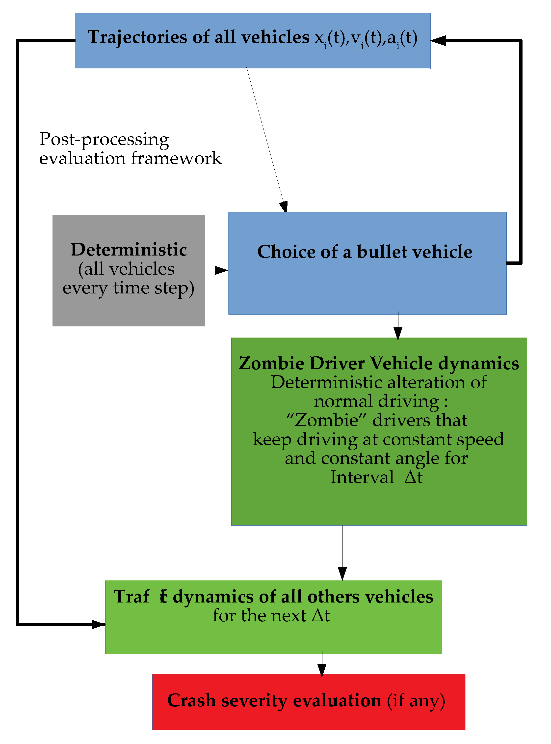
The whole Zombie Driver procedure is presented in Figure 4. The evaluation of crash severity of a potential impact is evaluated taking into account the speed and mass of the vehicles involved and by referring to the physical laws of conservation of momentum and energy conservation. According to Newton, the relative velocity of two bodies involved in a one-dimensional impact is directly proportional to the velocity, they had before the occurrence of the same impact, multiplied by a function coefficient elasticity of the bodies involved. Therefore, it is:
v 1 a v 2 a = ε ( v 1 b v 2 b )       w i t h       0 ε 1
  v 1 a and v 2 a represent the velocities of objects 1 and 2 after impact, while, v 1 b and v 2 b are the velocities of objects before impact. A totally inelastic impact corresponds to ε = 0 , on the contrary, the impact is elastic if ε = 1 . The Zombie Driver Software assumes that the collisions between the vehicles are inelastic and therefore if you consider the law of conservation of momentum in vector form it is possible to state that before the impact:
P = m 1 v 1 + m 2 v 2
m1 and m2 being the masses of the vehicles. It follows that the speed of the whole system after the impact is:
V = m 1 v 1 + m 2 v 2 m 1 + m 2
At this point it is possible to calculate the Δ V , which for the case of one-dimensional impact corresponds to:
Δ v 1 = V v 1       a n d     Δ v 2 = V v 2
The relative Δ V , instead, is:
Δ V 12 = v 2 v 1 = V Δ v 2 V + Δ v 1 = Δ v 1 Δ v 2
In addition, the kinetic energy of vehicles can be calculated before the occurrence of the accident, such as:
K a = 1 2 m 1 v 1 2 + 1 2 m 2 v 2 2
Still maintaining the inelastic impact hypothesis, the kinetic energy of the vehicles after the occurrence of the accident is equal to:
K b = 1 2 ( m 1 + m 2 ) V 2
The energy that develops during the impact can be evaluated as the difference between the two energies just evaluated and therefore is given by:
Δ K = K a K b = 1 2 m 1 v 1 2 + 1 2 m 2 v 2 2 1 2 ( m 1 + m 2 ) V 2 = 1 2 m r Δ V 12 2
with m r evaluated as:
m r = m 1 m 2 m 1 + m 2
Finally, it is also possible to establish the probability of deaths and injuries—with and without seatbelts—as a Δ V function, using the formulation suggested by Joksch [42]:
D e a d _ S e a t b e l t s = ( 0.621371 Δ V 69.18 ) 4.57
  D e a d _ N o S e a t b e l t s = ( 0.621371 Δ V 70.61 ) 3.54  
  I n j u r e d _ S e a t b e l t s = ( 0.621371 Δ V 67.43 ) 2.62  
  I n j u r e d _ N o S e a t b e l t s = ( 0.621371 Δ V 66.09 ) 2.22  
Synthesizing the extracted parameters are:
  • Total Energy: calculated as the sum of the energies of all impacts.
  • Maximum value of Energy among all impacts.
  • Total Δ V ( Δ V Total) as the sum of all Δ V of all simulated crashes.
  • Number of potential deaths: as the sum over all crashes of all probabilities of a death.
  • Number of injuries: as the sum over all crashes of all probabilities of an injury.
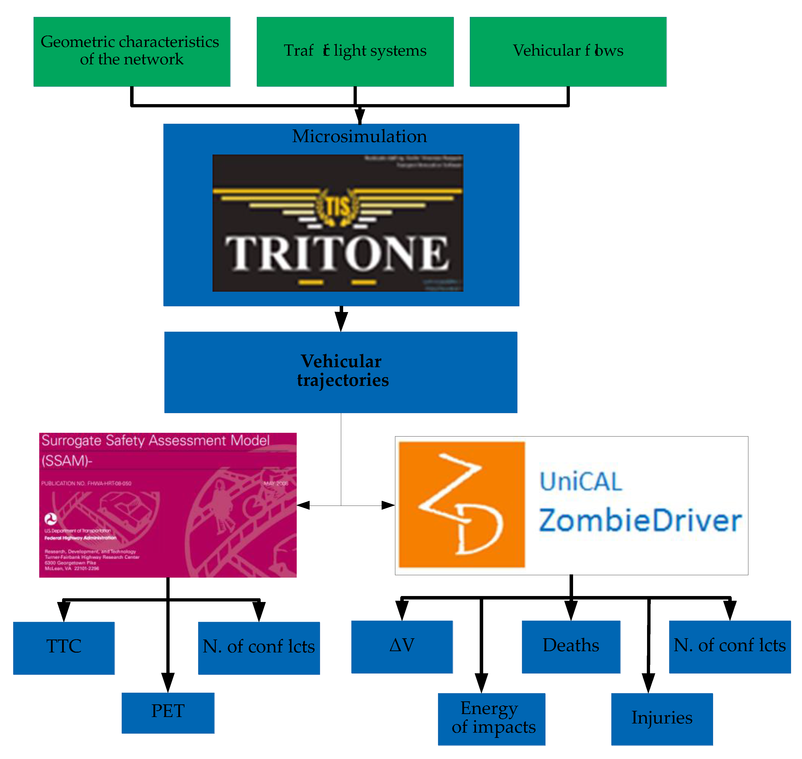
The flowchart of the whole procedure of applying Tritone and SSAM (embedded in Tritone) and Zombie Driver is depicted in Figure 5, where it is showed that the inputs are:
  • The geometric characteristics of the networks.
  • The characteristics of the traffic light systems.
  • The vehicular flows.

2.2. Case Studies

2.2.1. General Description of Two Case Studies

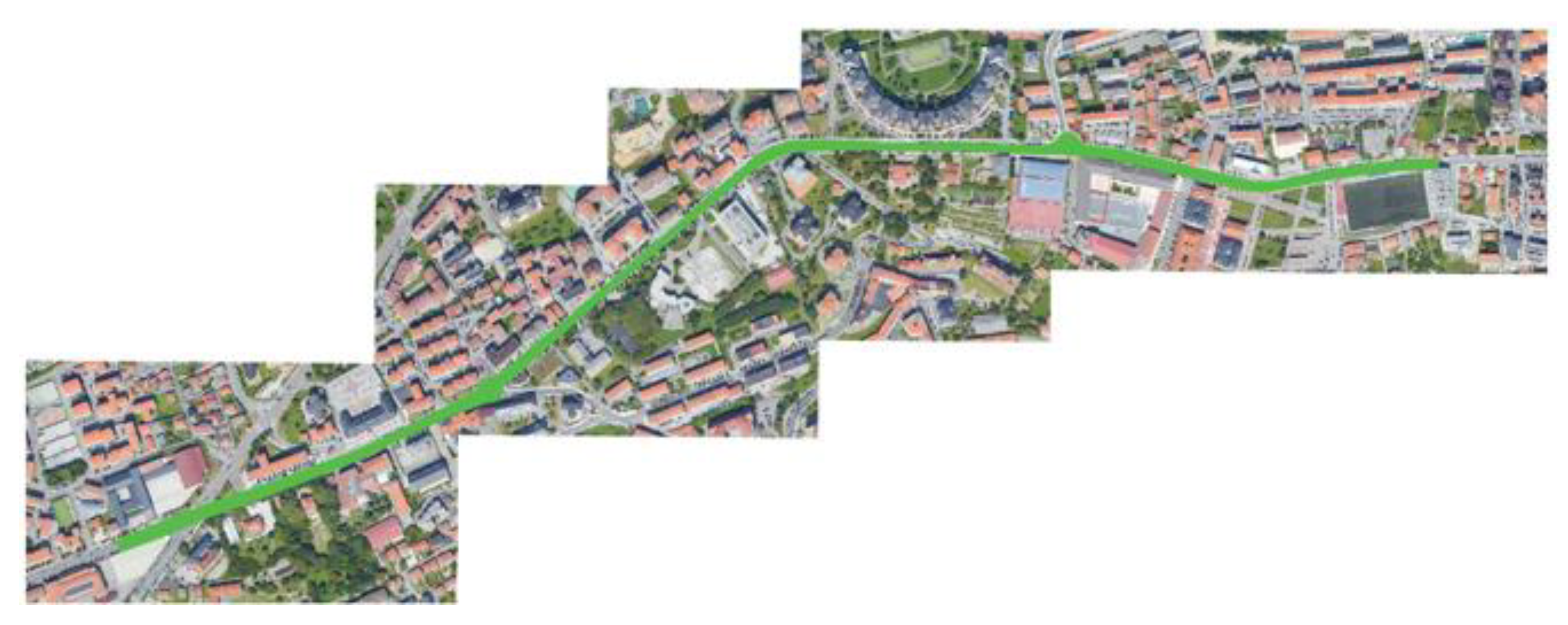
The Zombie Driver methodology was applied on two different case studies of the city of Santander (Spain): the area of Paseo de Pereda (Calle Jesús de Monasterio, Calle Calvo Sotelo, Paseo de Pereda and Calle Castelar) (Figure 6), located in the central area of the city of Santander and one of the busiest areas of the city, and the area of Paseo del General Dávila (Figure 7), located in the north of the same city—an area with average traffic throughout the day.
Both road networks extend for about 2 km and—with reference to the period of analysis—these areas have an excellent state of road maintenance and there is the presence of numerous poles of attraction along them. The first road network analysed consists of 27 entrances and/or exits and, inside it, were identified 12 cross-sections, two roundabout intersections and 14 road sections, there are 14 traffic light systems and 26 pedestrian crossings, many protected by traffic lights. The second road network, instead, as a whole has 24 entrances and/or exits, 11 cross-sections, two roundabout intersections and 15 road sections, there are seven traffic light systems and 27 pedestrian crossings, partly signalized. It is clear, therefore, that the two areas are very similar from the point of view of geometry, but they are substantially different from the point of view of vehicular traffic loads. In addition, the first network is located in an urban area while the second is located in a more peripheral, almost suburban area.
For both networks a modelling was created in the Tritone microsimulation environment. The data required for modelling are: the geometric characteristics of the networks, the characteristics of the traffic light systems and the vehicular flows. The analysed flows are derived from traffic surveys carried out over a whole month on the intermediate days of the week (Tuesday, Wednesday and Thursday: the so-called “average weekday”) in order to obtain an estimate of vehicular flows not influenced by special events such as weekends, commuter departures or returns, holidays, events, or temporary closures of network.

2.2.2. Time and Space Dimensions in the Two Case Studies

The study of the two networks differs not only in the amount of vehicular traffic present on the networks, but also in the time to which the surveys of the traffic flows refer. In fact, for the area of Paseo de Pereda we considered the temporal interval from 08:00 to 09:00, while for the area of Paseo del General Dávila we considered the temporal interval from 07:00 to 08:00.
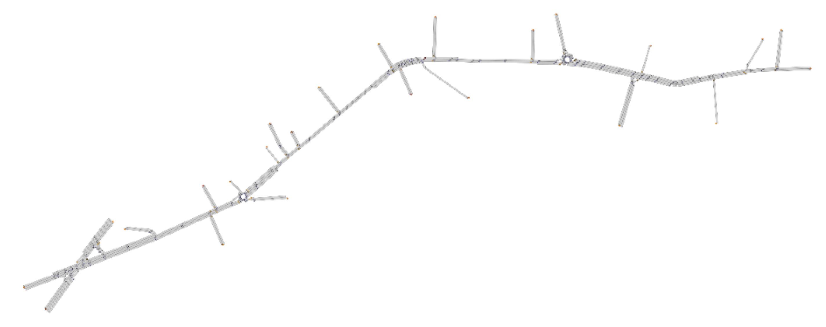
At the end of the modelling process, the geometry of the networks to be studied was created, which presents: 180 nodes, 364 arches, 14 traffic light systems and 96 lanterns, 4404 cars, eight buses and 87 heavy vehicles for the case study 1 (Figure 8); 302 nodes, 238 arches, seven traffic light systems and 61 lanterns, 1360 cars, 13 buses and nine heavy vehicles for the case study 2 (Figure 9).

2.2.3. Simulation Repetitions, Car Following Model and Calibration of the Microsimulation Model

The simulation of the networks is carried out in the Tritone Software adopting the Gipps model [43] (among the different possible options of Tritone) since it is commonly used (as an example in Aimsun [13] or in [44]). Each simulation is completely random in order to reflect reality better and, as a result, it is not enough to perform a single simulation to assess the state of a road network, but it is necessary to evaluate the data on a larger sample. For this reason, 30 simulations were completed for each scenario in order to minimize possible errors.
To verify the choice of using the Gipps model, it was decided to use the Geoffrey E. Havers G E H [45] calibration technique according to which:
G E H m a n e u v e r = 2 ( S i m u l a t e d R e a l ) 2 S i m u l a t e d + R e a l = { 1       i f       G E H m 5.0 0       i f       G E H m > 5.0
  G E H = m = 1 m a n . G E H m 85 %  
In both case studies, it was decided to compare the real data with the simulated data for 20 representative sections that covered the entire extent of the two areas analysed and it can be noted that for both networks the choice to use the Gipps model [43] is appropriate (Table 1 and Table 2) since the verification criteria are always satisfied.

2.2.4. The Comparative Analysis between Real Crash Data and Simulated Parameters

The objective of this document is to validate the Zombie Driver methodology described above and compare the methodology with classical indicators (TTC and PET). To this end, the analysed flows are derived from Automatic Traffic Counters deployed in the city and from traffic surveys carried out over a whole month. Real data on accidents in the city of Santander were taken into consideration in the two study areas between 2016 and 2018 extracted from the “Santander accident Police Database”. These data were located in the territory thanks to the presence of latitude and longitude values present in the database. After that, the road accidents were divided into categories: deaths, injuries and other types of accidents. The comparison between safety indicator parameters and real crash data was performed on a space grid. The Zombie Driver software is, in fact, able to create a grid on the study areas, whose mesh can take different sizes and define an origin so that each element of the mesh is characterized by an abscissa and an ordinate.
For each grid component on the basis of the trajectories the following parameters were calculated: maximum energy (maximum energy that can be generated in a collision and is distinguished in “generic”, “single” and “based on the collided object”); total energy (total energy that can be generated in a collision and is distinguished in “generic”, “single” and “based on the collided object”); vector speed difference total (sum of module of the vector difference between vehicle speed vectors during a collision); dead seatbelts (summation of the probability that a driver’s death will occur following a collision as a function of the difference between the vehicle speed vectors); injured seatbelts (summation of the probability that a driver’s injury will occur following a collision as a function of the difference between the vehicle speed vectors); dead + injured seatbelts (sum of dead seatbelts and injured seatbelts); collision (number of collisions occurring during the analysis of the network under study which can also be classified according to the angle of the deviated trajectory). In the application of this study, in order to calculate the above parameters, the following values were set: maximum distraction times 3 s; grid size 5 m; angle 15°.
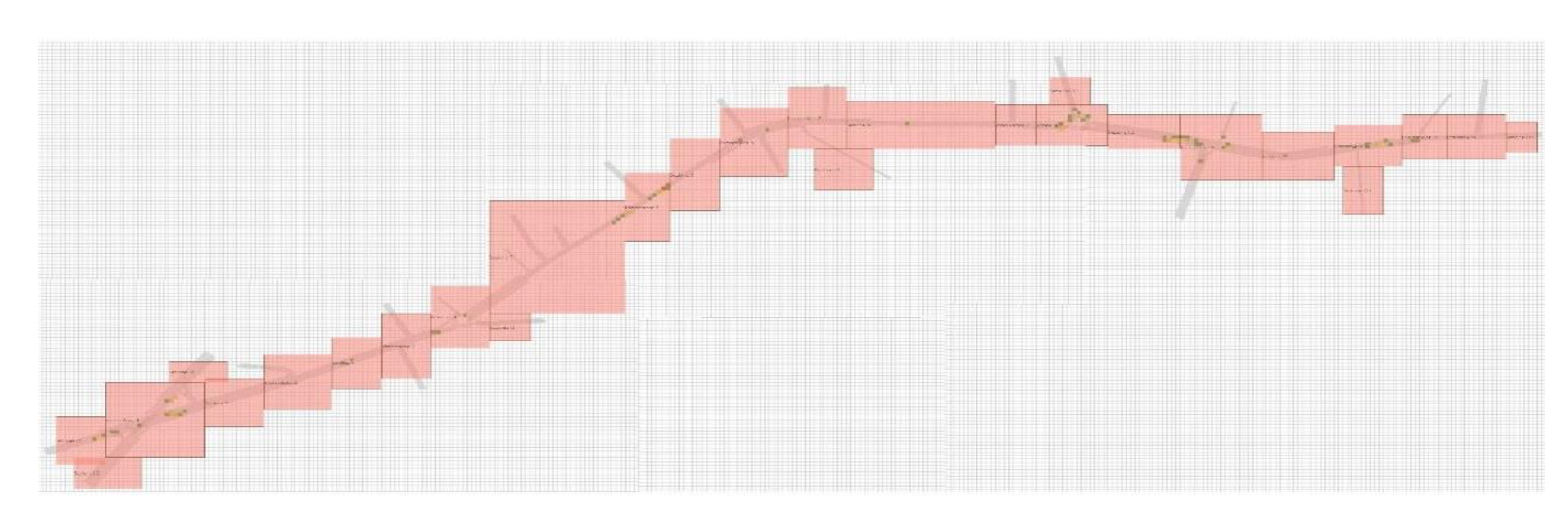
To make the real accident data comparable with the simulated data, a procedure for processing this data had to be developed. For this reason, it was decided to identify areas of influence starting from the intersections for both case studies. The remaining road sections were considered as road sections. The areas were plotted on the two networks using the Zombie Driver Software (Figure 10 and Figure 11) to facilitate the counting of simulated parameters falling within each area of influence.
For each area, the accidents that really happened were also counted, having their geolocation available. In this way, for case study 1, 12 intersections, 2 roundabout intersections and 14 road sections were identified, while for case study 2, 11 intersections, 2 roundabout intersections and 15 road sections were identified. It is therefore possible to identify data sets that are now finally comparable.

2.2.5. Real Accident Data

From the study on areas of influence, 287 total accidents can be detected in the case study 1 (Table 3) and 130 total accidents in the case study 2 (Table 4). In the following two tables the accident data are presented and the entering/exiting sections are identified with an "I" before the number.

2.2.6. Statistical Analysis

The statistical analysis was performed combining the real accident data of Table 3 and Table 4 with the simulated values of different kind of safety indicators to establish the validity of the proposed methodology in comparison with the more classic safety indicators obtained with the SSAM methodology: TTC, PET and the total number of conflicts. Statistical correlations have been assessed following the methodologies of Pearson [46] and Spearman [47]. Moreover, polynomial regression and a multiple linear regression have been proposed. The results of the statistical analysis are presented in the following section in different subsections relative to Pearson correlation, Spearman correlation, polynomial regression, multiple linear regression, polynomial regression and a graphical comparison of how every road area compares.

3. Results

The results obtained from the analysis of road safety and the comparison between real data and simulated data with reference to the two case studies are reported below.

3.1. Simulated Parameters with the Road Safety Analysis Methodology

Following the application of the methodology described in this document, and always with reference to the areas of influence, data series have been obtained (maximum energy “Energy Max”, total energy ”Energy Tot.”, vector speed difference total “∆V Tot.”, dead seatbelts “D”, injured seatbelts “I”, dead + injured seatbelts “D + I”, collision “Coll.”, Time to Collision SSAM “SSAM TTC”, Post-Encroachment Time SSAM “SSAM PET” and Conflicts SSAM “SSAM Confl.”) comparable with the real crash data (Table 5 and Table 6).

3.2. Comparative Analysis Real/Simulated

With all the real data and the simulated data, it was finally possible to compare them and, therefore, establish whether the Zombie Driver methodology can be reliably used to estimate crashes. Where a high correlation was established, the various simulated quantities were considered for a polynomial regression.
The statistical correlations considered for the Real/Simulated comparative analysis are those of Pearson [46] and Spearman [47].

3.2.1. Pearson Correlation

The Pearson correlation coefficient [46], if applied to two series of variables, makes it possible to understand whether there is a linear relationship between them. It takes values between –1 and +1. The closer the coefficient is to –1 or to +1, the higher the correspondence between the variables, while in the case in which the coefficient tends to 0 there is a complete absence of linearity relationships between the variables. The index is calculated through the following equation:
ρ x y = σ x y σ x σ y
where x and y represent the statistical variables taken into consideration, σ x y represents the value of the covariance between x and y , σ x represents the standard deviation of variable x , and σ y represents the standard deviation of variable y .
Twelve pairs of variables were defined keeping the “Real accident total” series fixed, each time varying the series of simulated parameters. In this way, it was possible to calculate the Pearson coefficient for the pairs of real/simulated variables in order to establish which simulated parameters demonstrated the best correlations with the real parameters (Table 7 and Table 8).

3.2.2. Spearman Correlation

The Spearman correlation coefficient [47] assesses the correlation that may exist between two statistical variables by reference to the rank of the series to be compared. The coefficient is calculated by applying a particular formulation of the Pearson coefficient [46]:
ρ = i ( x i x a v e r a g e ) ( y i y a v e r a g e ) i ( x i x a v e r a g e ) 2 i ( y i y a v e r a g e ) 2
where x and y represent the statistical variables taken into consideration, x a v e r a g e represents the average of variable x , and y a v e r a g e represents the average of variable y .
Furthermore, for the calculation of the Spearman coefficient, twelve pairs of variables were identified, keeping the “Real accident total” series fixed and varying the series of simulated parameters (Table 9 and Table 10).

3.2.3. Polynomial Regression

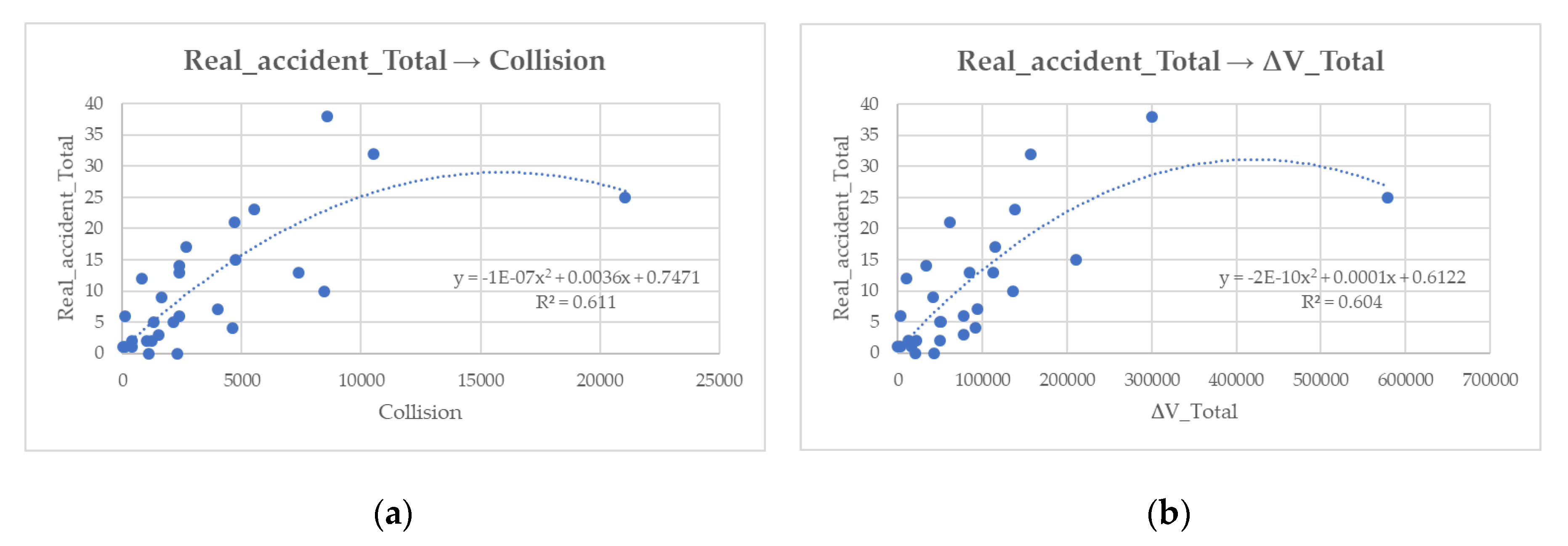
To investigate the real/simulated analysis further, a polynomial (second degree) regression was applied to the pairs of series that showed better correlations. The aim of this simple polynomial regression was to establish a methodology that can estimate the number of accidents in a given area with the simulation, results of our methodology. Similar attempts have been carried out in other works such as: [12,48,49].
For case study 1, the serial pairs that were considered were Real accident total-Collision, and Real accident total-∆V Total (Figure 12). For case study 2, the serial pairs that were considered were, instead, Real accident total-Dead + Injured, and Real accident total-Dead Seatbelts (Figure 13).
Both polynomial regressions for case studies 1 and 2 show an increasing tendency in the resulting curves. The chosen indicators seem to well anticipate the number of accidents. In case study 2, there was one area where both the total number of collisions and the ∆V Total were much higher than in other areas of the network. Removal of this value would have increased the correlation factor R2 (which was 0.61 for Collision and 0.60 for ∆V Total). It was decided not to remove outliers in this case and in other cases of the above described Pearson and Spearman analysis, since practically all the values of all parameters were contained in the interval created by subtracting and adding three times the standard deviation to the average value.

3.2.4. Multiple Linear Regression

The multiple linear regression is a development of simple linear regression, the only difference with the latter being that there are more independent variables that define a dependent variable. For case study 1, the chosen dependent variable is the number of accidents while the chosen independent variables are: total energy (MJ), vector speed difference total (km/s), dead seatbelts (-), injured seatbelts (-) and collision (-).
A c c i d e n t C a s e   s t u d y   1 = 3.0039 1.39 · 10 6 E n e r g y T o t a l + 5.6368 Δ V T o t a l + 0.1598 D e a d S e a t b e l t s + 0.0540 I n j u r e d S e a t b e l t s 0.0115 C o l l i s i o n
This regression has an R fitting of 0.5878.
Furthermore, for case study 2, the chosen dependent variable is the number of accidents, and the independent variables chosen are: total energy (MJ), vector speed difference total (km/s), dead seatbelts (-), injured seatbelts (-) and collision (-).
A c c i d e n t C a s e   s t u d y   2 = 1.5640 4.66 · 10 7 E n e r g y T o t a l + 2.2760 Δ V T o t a l + 0.1899 D e a d S e a t b e l t s 0.0831 I n j u r e d S e a t b e l t s 0.0021 C o l l i s i o n
This regression has an R fitting of 0.5686.

3.2.5. Graphical Comparison of Ranks

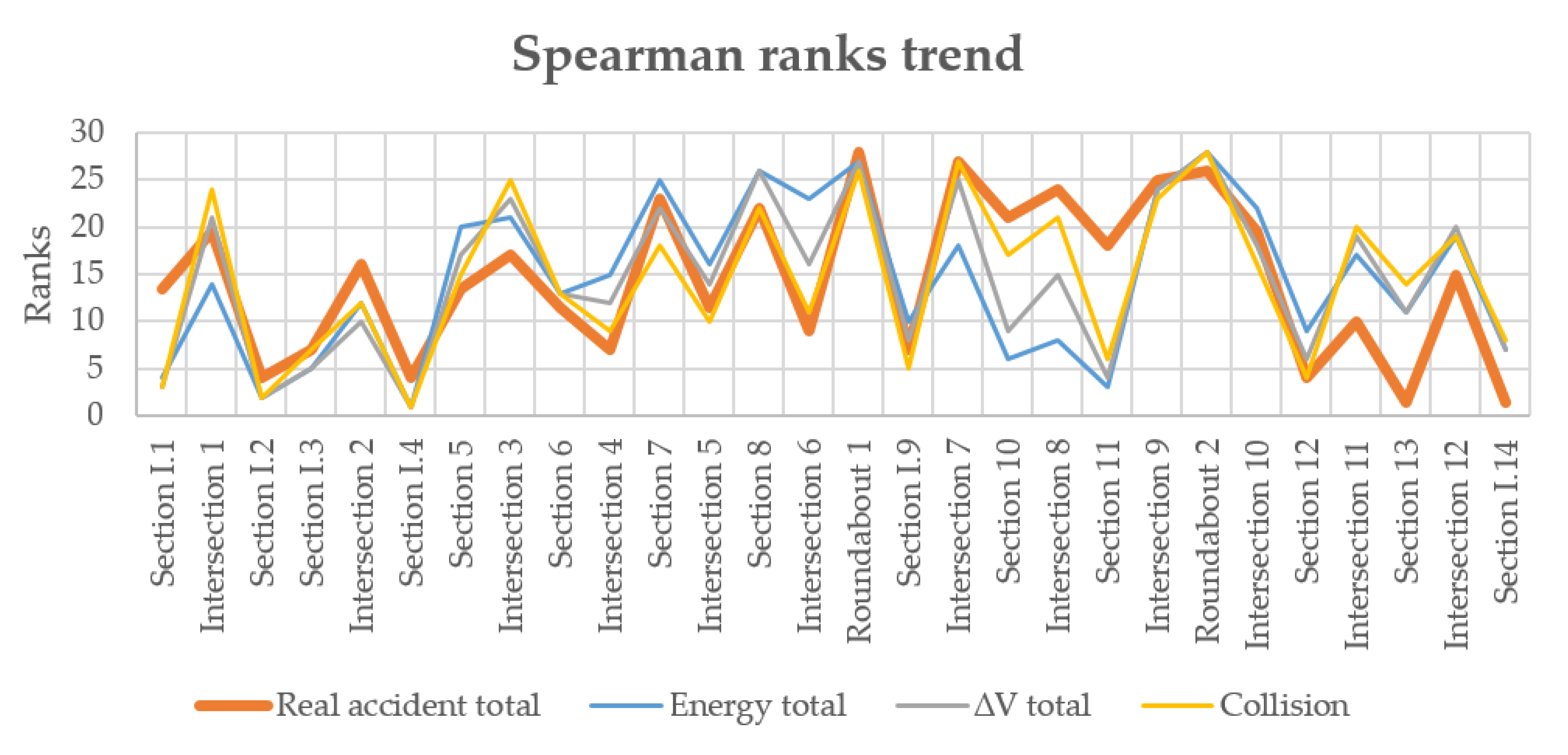
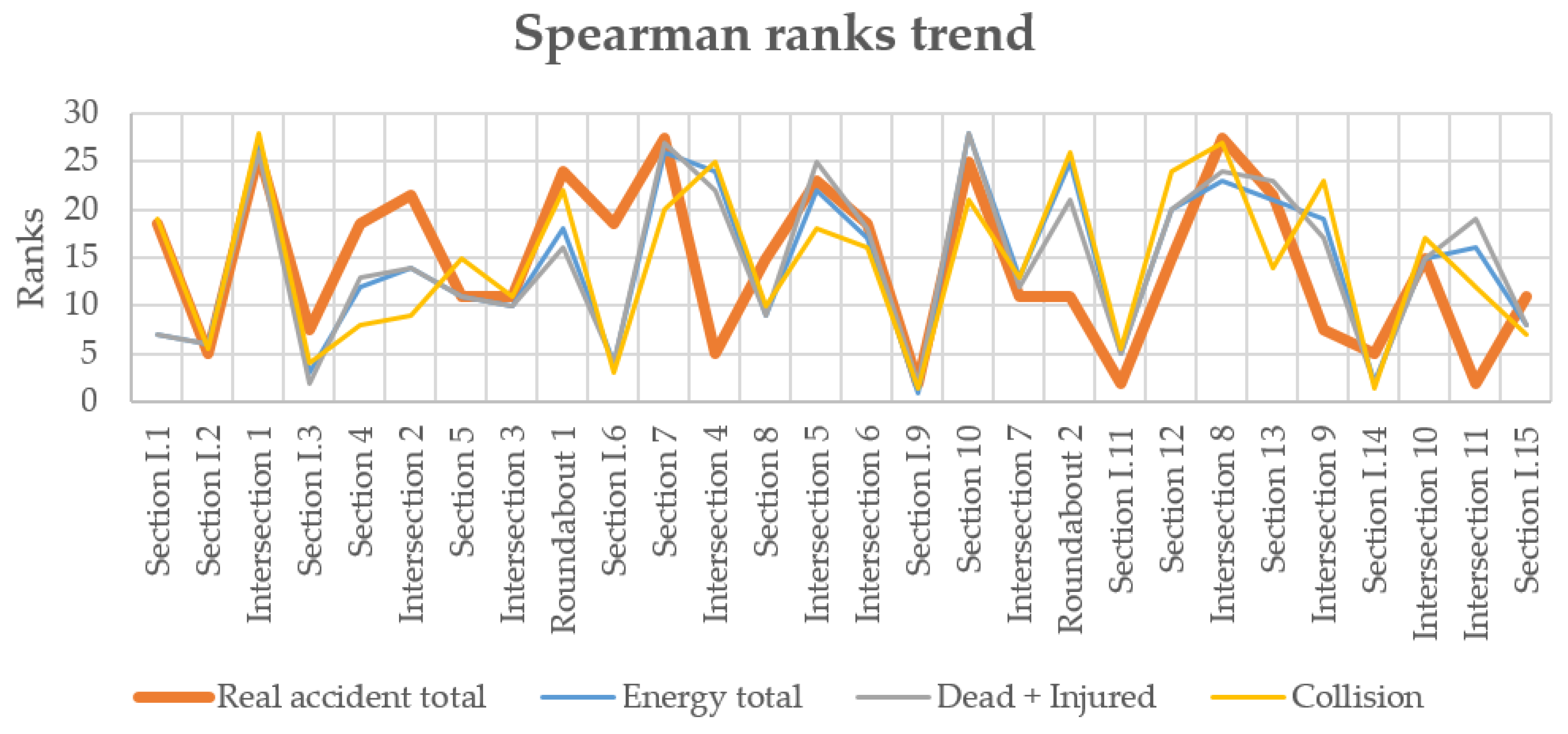
Below is the graphical comparison of the ranks between the series of accidents recorded on-site and the series of simulated parameters descending from the calculation of the Spearman correlation for the two case studies (Figure 14 and Figure 15). In the figures for each intersection or road section, it is indicated how it ranks in terms of real accident data and three different simulated parameters. This graphical comparison can help establish—at a glance—the capacity of the best three indicators for each case study to identify potential black spots. The parameters that are considered in Figure 14 relative to case study 1 are: Energy total, ∆V Total and Collision. The parameters that are considered in Figure 15 relative to case study 2 are: Energy total, Dead + Injured and Collision.

4. Discussion

The first statistical analysis that was conducted with Spearman and Pearson methodologies was able to establish the best indicators according to the given data.
The results of the proposed methodology show a good correlation between simulated parameters and the real crash data with both the Pearson [46] and the Spearman [47] index. The results are noticeably better than those obtained with other classical conflict-based indicators extracted from SSAM software such as TTC and PET.
In case study 1, the parameters that showed better correlation (both of Pearson [20] and of Spearman [47]) turn out to be ∆V total and collision; instead, in case study 2, the parameters that are best correlated to the real data are those related to the number of deaths and the number of injuries. This stems from the fact that the area of Paseo de Pereda is an urban area where vehicles are very close to each other. This condition favours the onset of probable conflicts as they are determined precisely by the distance (spatial and temporal) between vehicles. Contrastingly, the area of Paseo del General Dávila, being a more peripheral and less busy area, leads to vehicles achieving higher speeds, and this is evidenced by the fact that all the parameters that showed the best correlations are all derived from ∆V.
The study discussed in this document was carried out on two different areas of study in order to differentiate the analysis of accidents as much as possible and to obtain a validation of the method on more than one scenario. This work also applied a multiple linear regression, which allowed us to derive the Equations (18) and (19)—useful for the estimation of accidents.
It is possible to notice how the series of the simulated parameters follows the trend of the series of the real data in the two cases well; therefore, the Zombie Driver methodology shows a moderate correlation to the real observed data for both networks. This correlation is much better than what has been obtained with the classical indicators calculated with the SSAM methodology.
The poor correlation between the three indicators calculated with the SSAM methodology is noticeable in this work, and possibly evidences a conceptual limit of currently used surrogate safety performance indicators. The classical theory of conflicts does consider the existence of a conflict, though only when two vehicles are driving on conflicting trajectories. Vehicles that are travelling in opposite directions on a two-way single carriageway do not generate any conflict. In our network, there were many lanes for direction and intense traffic. Despite this dangerous layout that actually produced many accidents, there were many road areas (sections) in which there was not even one conflict according to SSAM methodology.
This result is the most important result of this paper, and—if confirmed by other works conducted on the same road network or similar road networks (where many parallel lanes share a two-way single carriageway)—it may suggest a restriction for the field of applicability of indicators such as TTC.
Regarding the presented Zombie Driver methodology, the ∆V parameter has a good ranking in terms of correlation in both case studies, despite the different conditions that exist on the two networks. It can be stated that the ∆V parameter represents the most reliable surrogate safety indicator according to this work. This result is in accordance with recent studies that have proposed an evolution from traditional traffic safety indicators that can be obtained from SSAM software [20]. This new direction of research suggests, in fact, the use of indicators that consider the severity of potential crashes.
The results of this paper are based on two simple networks for a total simulated distance of 3.6 km. The results are not sufficient to draw out a definitive conclusion on classical surrogate safety indicators. More research efforts can be devoted to confirm the presented results and better calibrate the Zombie Driver procedure (or any other procedure that introduces random deviation in vehicle trajectories). Despite the limitations of this work, we can conclude, that the presented results for decision-makers imply that there is a need to apply (with great caution) microsimulation and classical surrogate safety indicators for situations where an economical assessment of different road sections is requested.
Microsimulation can be a great tool for helping in decisions on exactly what safety requalification interventions can be programmed, but more research is yet to be carried out before this becomes an established methodology.
5. Conclusions

A new methodology to assess traffic safety levels using traffic microsimulation has been developed and applied in a real traffic scenario. The methodology simulates potential crashes starting from the knowledge of vehicular trajectories extrapolated from microsimulation. Real accident data were used to test this methodology and other classical methodologies, which are also based on conflict indicators. Results show that the proposed methodology performs better than other commonly used indicators in both of the simulated traffic networks. More research is necessary to conclude that our methodology is universally applicable. However, this paper gives interesting insights into the use of traffic conflict methodologies in microsimulation, which could help to develop better traffic conflict indicators. The evaluation of traffic safety with microsimulation may become an important tool for engineers in the future, since it could assist in identifying the more promising interventions in terms of both road safety and traffic congestion.

Supplementary Materials

The software Zombie Driver can be downloaded for free and applied on trajectories extracted from SSAM software at: http://tis.unical.it/.

Author Contributions

V.A. and V.P.G. were responsible for conceptualization and methodology; V.P.G. carried on all the software development. B.A., L.D., G.G. and A.V. performed supervision, review and editing. M.M. and W.S. carried on the simulations and the statistical analysis. All authors have read and agreed to the published version of the manuscript.

Funding

This study and the development of future research are possible thanks to financing from the Santander City Council from the SMARTRANSPORT project.

Conflicts of Interest

The authors declare no conflict of interest.

References

  1. Hauer, E. On the estimation of the expected number of accidents. Accid. Anal. Prev. 1986. [Google Scholar] [CrossRef]
  2. Jovanis, P.P.; Chang, H.-L. Modeling the relationship of accidents to miles traveled. Transp. Res. Board 1986, 1068, 42–51. [Google Scholar]
  3. Miaou, S.P.; Lum, H. Modeling vehicle accidents and highway geometric design relationships. Accid. Anal. Prev. 1993. [Google Scholar] [CrossRef]
  4. Miaou, S.P. The relationship between truck accidents and geometric design of road sections: Poisson versus negative binomial regressions. Accid. Anal. Prev. 1994. [Google Scholar] [CrossRef] [Green Version]
  5. Shankar, V.; Mannering, F.; Barfield, W. Effect of roadway geometrics and environmental factors on rural freeway accident frequencies. Accid. Anal. Prev. 1995. [Google Scholar] [CrossRef]
  6. Hauer, E. Observational before/after Studies in Road Safety: Estimating the Effect of Highway and Traffic Engineering Measures on Road Safety; Emerald Publishing: Bingley, UK, 1997; ISBN 9780080430539. [Google Scholar]
  7. Abdel-Aty, M.A.; Radwan, A.E. Modeling traffic accident occurrence and involvement. Accid. Anal. Prev. 2000. [Google Scholar] [CrossRef]
  8. Yan, X.; Radwan, E.; Abdel-Aty, M. Characteristics of rear-end accidents at signalized intersections using multiple logistic regression model. Accid. Anal. Prev. 2005, 37, 983–995. [Google Scholar] [CrossRef]
  9. Hydén, C. The Development of a Method for Traffic Safety Evaluation: The Swedish Traffic Conflict Technique. Bulletin/Lund Institute of Technology, Department of Traffic Planning and Engineering; Tekniska Högskolan i Lund: Lund, Sweden, 1987. [Google Scholar]
  10. Hayward, J. Near Misses as a Measure of Safety at Urban Intersections. Ph.D. Thesis, Department of Civil and Environmental Engineerin, Pennsylvania State University, State College, PA, USA, 1971. [Google Scholar]
  11. Allen, B.L.; Shin, B.T.; Cooper, P. Analysis of traffic conflicts and collisions. Transp. Res. Rec. 1978, 67–74. [Google Scholar]
  12. Gettman, D.; Sayed, T.; Pu, L.; Shelby, S. Surrogate Safety Assessment Model and Validation; Federal Highway Administration: Washington, DC, USA, 2008.
  13. Barceló, R.G.; Ferrar, J.L.; Grau, R. AIMSUN2 and the GETRAM Simulation Enviromen; Technical Report; Departamento de Estadística e Investigación Operativa. Universidad Politécnica de Cataluña: Barcelona, Spain, 1994. [Google Scholar]
  14. PTV Group. PTV Vissim 7 User Manual; PTV AG: Karlsruhe, Germany, 2015. [Google Scholar]
  15. Cameron, G.D.B.; Duncan, G.I.D. PARAMICS—Parallel microscopic simulation of road traffic. J. Supercomput. 1996, 10, 25–53. [Google Scholar] [CrossRef]
  16. Surrogate Safety Assessment Model Overview. Available online: https://cms7.fhwa.dot.gov/research/safety/ssam/surrogate-safety-assessment-model-overview (accessed on 23 January 2020).
  17. Sohel Mahmud, S.M.; Ferreira, L.; Hoque, S.; Tavassoli, A. Application of proximal surrogate indicators for safety evaluation: A review of recent developments and research needs. IATSS Res. 2017. [Google Scholar] [CrossRef]
  18. Young, W.; Sobhani, A.; Lenné, M.G.; Sarvi, M. Simulation of safety: A review of the state of the art in road safety simulation modelling. Accid. Anal. Prev. 2014. [Google Scholar] [CrossRef]
  19. Zheng, L.; Ismail, K.; Meng, X. Traffic conflict techniques for road safety analysis: Open questions and some insights. Can. J. Civ. Eng. 2014. [Google Scholar] [CrossRef]
  20. Laureshyn, A.; De Ceunynck, T.; Karlsson, C.; Svensson, Å.; Daniels, S. In search of the severity dimension of traffic events: Extended Delta-V as a traffic conflict indicator. Accid. Anal. Prev. 2017. [Google Scholar] [CrossRef] [Green Version]
  21. Laureshyn, A.; Svensson, Å.; Hydén, C. Evaluation of traffic safety, based on micro-level behavioural data: Theoretical framework and first implementation. Accid. Anal. Prev. 2010. [Google Scholar] [CrossRef]
  22. Ivan, J.N.; Konduri, K.C. Chapter 15. Crash Severity Methods. In Safe Mobility: Challenges, Methodology and Solutions; Emerald Group Publishing: Bingley, UK, 2018; pp. 325–350. [Google Scholar]
  23. Mannering, F.L.; Lee, J. Analysis of Roadside Accident Frequency and Severity and Roadside Safety Management; Washington State Transportation Center: Seattle, WA, USA, 1999. [Google Scholar]
  24. National Highway Traffic Safety Administration. Traffic Safety Facts: 2015; Report DOT HS 812 384; National Highway Traffic Safety Administration, National Center for Statistics and Analysis, U.S. Department of Transportation: Washington, DC, USA, 2017.
  25. Van Treese, J. Frequency and severity of tree and other object crashes in Florida from 2006 to 2013. In Proceedings of the Trees, People and the Build Environment, Birmingham, UK, 5–6 April 2017. [Google Scholar]
  26. Marzano, V.; Tocchi, D.; Papola, A.; Aponte, D.; Simonelli, F.; Cascetta, E. Incentives to freight railway undertakings compensating for infrastructural gaps: Methodology and practical application to Italy. Transp. Res. Part A Policy Pract. 2018. [Google Scholar] [CrossRef]
  27. Astarita, V.; Florian, M.; Musolino, G. A microscopic traffic simulation model for the evaluation of toll station systems. In Proceedings of the IEEE Conference on Intelligent Transportation Systems, ITSC, Oakland, CA, USA, 25–29 August 2001. [Google Scholar]
  28. Astarita, V.; Giofré, V.; Guido, G.; Vitale, A. Investigating road safety issues through a microsimulation model. Procedia Soc. Behav. Sci. 2011, 20, 226–235. [Google Scholar] [CrossRef] [Green Version]
  29. Astarita, V.; Giofré, V.P. From traffic conflict simulation to traffic crash simulation: Introducing traffic safety indicators based on the explicit simulation of potential driver errors. Simul. Model. Pract. Theory 2019, 94, 215–236. [Google Scholar] [CrossRef]
  30. Osorio, C.; Punzo, V. Efficient calibration of microscopic car-following models for large-scale stochastic network simulators. Transp. Res. Part B Methodol. 2019. [Google Scholar] [CrossRef]
  31. Martinez, F.J.; Toh, C.K.; Cano, J.C.; Calafate, C.T.; Manzoni, P. A survey and comparative study of simulators for vehicular ad hoc networks (VANETs). Wirel. Commun. Mob. Comput. 2011. [Google Scholar] [CrossRef]
  32. Gentilea, G. New formulations of the stochastic user equilibrium with logit route choice as an extension of the deterministic model. Transp. Sci. 2018. [Google Scholar] [CrossRef]
  33. Gentile, G. Solving a Dynamic User Equilibrium model based on splitting rates with Gradient Projection algorithms. Transp. Res. Part B Methodol. 2016. [Google Scholar] [CrossRef]
  34. Cantarella, G.E.; Di Febbraro, A.; Di Gangi, M.; Giannattasio, O. Stochastic Multi-Vehicle Assignment to Urban Transportation Networks. In Proceedings of the MT-ITS 2019—6th International Conference on Models and Technologies for Intelligent Transportation Systems, Kraków, Poland, 5–7 June 2019. [Google Scholar]
  35. Cantarella, G.E.; Watling, D.P. A general stochastic process for day-to-day dynamic traffic assignment: Formulation, asymptotic behaviour, and stability analysis. Transp. Res. Part B Methodol. 2016. [Google Scholar] [CrossRef]
  36. Trozzi, V.; Gentile, G.; Kaparias, I.; Bell, M.G.H. Effects of Countdown Displays in Public Transport Route Choice Under Severe Overcrowding. Netw. Spat. Econ. 2015. [Google Scholar] [CrossRef] [Green Version]
  37. Kucharski, R.; Gentile, G. Simulation of rerouting phenomena in Dynamic Traffic Assignment with the Information Comply Model. Transp. Res. Part B Methodol. 2019, 126, 414–441. [Google Scholar] [CrossRef]
  38. Marzano, V.; Papola, A.; Simonelli, F.; Papageorgiou, M. A Kalman Filter for Quasi-Dynamic o-d Flow Estimation/Updating. IEEE Trans. Intell. Transp. Syst. 2018. [Google Scholar] [CrossRef]
  39. Papola, A.; Tinessa, F.; Marzano, V. Application of the Combination of Random Utility Models (CoRUM) to route choice. Transp. Res. Part B Methodol. 2018. [Google Scholar] [CrossRef]
  40. Papola, A. A new random utility model with flexible correlation pattern and closed-form covariance expression: The CoRUM. Transp. Res. Part B Methodol. 2016. [Google Scholar] [CrossRef]
  41. Giofrè, V.P. Sviluppo di un Modello di Microsimulazione del Traffico Traffico. Master’s Thesis, University of Calabria, Rende, Italy, 2010. [Google Scholar]
  42. Joksch, H.C. Velocity change and fatality risk in a crash-A rule of thumb. Accid. Anal. Prev. 1993. [Google Scholar] [CrossRef]
  43. Gipps, P.G. A behavioural car-following model for computer simulation. Transp. Res. Part B 1981. [Google Scholar] [CrossRef]
  44. Kim, J.; Mahmassani, H.S. Correlated parameters in driving behavior models: Car-following example and implications for traffic microsimulation. Transp. Res. Rec. 2011. [Google Scholar] [CrossRef] [Green Version]
  45. Highway Agency. Traffic Appraisal of Road Schemes, Section 2.5, Part I, Traffic Appraisal in Urban Areas. In Design Manual for Roads and Bridges; The Stationery Office: London, UK, 1996; Volume 12. [Google Scholar]
  46. Pearson, K. Notes on regression and inheritance in the case of two parents. Proc. R. Soc. 1895, 58, 240–242. [Google Scholar]
  47. Spearman, C. The Proof and Measurement of Association between Two Things. Am. J. Psychol. 1987, 100, 441. [Google Scholar] [CrossRef]
  48. Dijkstra, A.; Marchesini, P.; Bijleveld, F.; Kars, V.; Drolenga, H.; van Maarseveen, M. Do Calculated Conflicts in Microsimulation Model Predict Number of Crashes? Transp. Res. Rec. 2010. [Google Scholar] [CrossRef]
  49. Shahdah, U.; Saccomanno, F.; Persaud, B. Integrated traffic conflict model for estimating crash modification factors. Accid. Anal. Prev. 2014. [Google Scholar] [CrossRef]
Figure 1. Hydén pyramid.
Sustainability 12 00925 g001
Figure 2. Surrogate safety indicator: TTC.
Sustainability 12 00925 g002
Figure 3. Surrogate safety indicator: PET.
Sustainability 12 00925 g003
Figure 4. The Zombie Driver procedure.
Sustainability 12 00925 g004
Figure 5. The whole procedure.
Sustainability 12 00925 g005
Figure 6. Case study 1: area of Paseo de Pereda, Santander (Spain).
Sustainability 12 00925 g006
Figure 7. Case study 2: area of Paseo del General Dávila, Santander (Spain).
Sustainability 12 00925 g007
Figure 8. Case study 1: road network modelling.
Sustainability 12 00925 g008
Figure 9. Case study 2: road network modelling.
Sustainability 12 00925 g009
Figure 10. Case study 1: areas of influence.
Sustainability 12 00925 g010
Figure 11. Case study 2: areas of influence.
Sustainability 12 00925 g011
Figure 12. Case study 1, second degree polynomial regression: (a) Real accident total–Collision; (b) Real accident total–∆V Total.
Sustainability 12 00925 g012
Figure 13. Case study 2, second degree polynomial regression: (a) Real accident total-Dead + Injured; (b) Real accident total-Dead Seatbelts.
Sustainability 12 00925 g013
Figure 14. Case study 1: Spearman ranks trend.
Sustainability 12 00925 g014
Figure 15. Case study 2: Spearman ranks trend.
Sustainability 12 00925 g015
Table 1. Case study 1: calibration of the model with the GEH technique [45].
Case Study 1
Control SectionReal FlowSimulated FlowGEHCheck
12252260.0671
24913158.7670
36996003.8851
45315150.7001
56978254.6401
64234772.5461
77038384.8631
84404791.8191
98168922.6011
104634820.8741
11144613831.6751
12132798110.1850
13147513812.4881
14119679612.6740
153393510.6461
167809004.1401
177962502.7841
187328243.2981
1913012000.8941
204125094.5201
GEH85.00%VERIFIED
Table 2. Case study 2: calibration of the model with the GEH technique [45].
Case Study 2
Control SectionReal FlowSimulated FlowGEHCheck
11692253.9901
21912423.4661
31461923.5381
42252722.9811
51471923.4561
62432721.8071
71462044.3841
83182851.9011
91902272.5621
104753923.9861
111302015.5190
123453052.2191
131622133.7251
143483052.3801
151182388.9940
161461923.5381
172402722.0001
181642385.2200
193753183.0621
203473052.3261
GEH85.00%VERIFIED
Table 3. Case study 1: real accident.
Case Study 1
ID.DeadInjuredOtherTotal
Section I.11236
Intersection 1031013
Section I.20011
Section I.30022
Intersection 20279
Section I.40011
Section 50156
Intersection 303710
Section 60325
Intersection 40202
Section 726917
Intersection 50145
Section 8041115
Intersection 60123
Roundabout 10102838
Section I.90022
Intersection 70131932
Section 1005914
Intersection 8071421
Section 1106612
Intersection 9081523
Roundabout 2281525
Intersection 1004913
Section 120101
Intersection 110134
Section 130000
Intersection 120167
Section I.140000
Table 4. Case study 2: real accident.
Case Study 2
ID.DeadInjuredOtherTotal
Section I.10415
Section I.20101
Intersection 107310
Section I.30112
Section 40235
Intersection 20246
Section 50033
Intersection 30123
Roundabout 10358
Section I.60145
Section 7051015
Intersection 40011
Section 80224
Intersection 50167
Intersection 60325
Section I.90000
Section 101449
Intersection 70033
Roundabout 20213
Section I.110000
Section 120314
Intersection 816815
Section 131416
Intersection 90112
Section I.140101
Intersection 100134
Intersection 110000
Section I.151113
Table 5. Case study 1: simulated parameters.
Case Study 1
ID.Energy∆V Tot.Dead and Injured 1Coll.SSAM
MaxTot.DID + ITTCPETConfl.
(MJ)(MJ)(km/s)(0–1)(0–1)(0–1)(-)(s)(s)(-)
S I.10.53.80.8913221211.112.061
I 11.670.731.14716220973811.172.042421
S I.20.61.90.70331021.041.951
S I.30.85.53.5191010301.162.05406
I 25.449.111.59816626416401.222.10262
S I.40.20.10.0000121.192.003
S 55.2102.521.721235857023731.111.95621
I 37.0111.137.717432649984631.091.931935
S 64.157.413.913020333321271.121.88493
I 45.878.913.919829749612151.152.0485
S 76.0185.331.8526730125626801.041.86396
I 55.579.114.119828848613141.182.08143
S 86.7350.058.69441329227347531.141.991150
I 66.4134.521.636150886915001.191.9961
R 16.4364.383.45581116167485571.232.06256
S I.96.537.16.0931372304161.252.0220
I 72.385.143.53917621510,5111.172.032602
S 105.811.99.11161723881.252.02184
I 87.324.116.95404547131.192.081626
S 110.42.92.80338061.172.1028
I 96.0179.438.6462662112455351.232.11716
R 26.0631.0160.99111877278821,0541.091.911018
I 105.4113.823.425240165323761.202.12449
S 125.325.44.566941603980.000.000
I 116.080.325.612823836546111.232.051172
S 132.538.811.87212419623041.141.96340
I 126.093.226.015528844239731.111.991259
S I.144.419.05.630548410851.232.06342
1 Calculated using Joksch’s formulas [42] in the condition of seatbelts.
Table 6. Case study 2: simulated parameters.
Case Study 2
ID.Energy∆V Tot.Dead and Injured 1Coll.SSAM
MaxTot.DID + ITTCPETConfl.
(MJ)(MJ)(km/s)(0–1)(0–1)(0–1)(-)(s)(s)(-)
S I.10.65.92.4816245090.000.00402
S I.22.90.70.1124130.000.000
I 17.358.517.49518127526401.172.061618
S I.30.10.10.0000100.000.000
S 40.616.92.26263126820.000.000
I 28.919.42.46971140910.000.000
S 51.412.62.63745832961.152.06264
I 30.711.22.03444781471.272.176
R 11.627.86.458951536651.242.05421
S I.60.30.10.001130.000.000
S 71.557.38.71892134035731.172.0587
I 42.352.713.46516022516011.132.04370
S 82.49.81.52633591111.172.019
I 53.037.35.31261352613801.172.2236
I 63.227.24.174901633251.181.9874
S I.90.00.00.000000.000.000
S 100.767.59.92122464586471.222.02211
I 70.918.12.950671171771.242.111
R 23.054.614.36715121818191.142.04596
S I.110.20.40.1112131.142.0010
S 120.534.59.27111818913461.262.03563
I 81.051.613.78116324418881.162.031014
S 130.534.95.31021402412880.000.000
I 91.229.97.7619916010901.141.97657
S I.140.00.00.000000.000.000
I 101.222.94.356871433371.262.0512
I 110.526.03.9791081871480.000.000
S I.150.56.61.0212848340.000.000
1 Calculated using Joksch’s formulas [42] in the condition of seatbelts.
Table 7. Case study 1: Pearson correlation coefficient.
Case Study 1
Param.Energy∆V Tot.Dead and Injured 1Coll.SSAM
MaxTot.DID + ITTCPETConfl.
Real accident total0.260.600.670.480.560.530.690.200.200.46
Ranking83264519107
1 Assuming seatbelts.
Table 8. Case study 2: Pearson correlation coefficient.
Case Study 2
Param.Energy∆V Tot.Dead and Injured 1Coll.SSAM
MaxTot.DID + ITTCPETConfl.
Real accident total0.260.630.530.670.650.670.430.320.330.44
Ranking10452317986
1 Assuming seatbelts.
Table 9. Case study 1: Spearman correlation coefficient.
Case Study 1
Param.Energy∆V Tot.Dead and Injured 1Coll.SSAM
MaxTot.DID + ITTCPETConfl.
Real accident total0.380.580.730.400.520.480.790.100.210.54
Ranking83275611094
1 Assuming seatbelts.
Table 10. Case study 2: Spearman correlation coefficient.
Case Study 2
Param.Energy∆V Tot.Dead and Injured 1Coll.SSAM
MaxTot.DID + ITTCPETConfl.
Real accident total0.440.580.520.640.570.610.500.350.300.38
Ranking73514269108
1 Assuming seatbelts.