Spatial Heterogeneity of the Impact Factors on Gray Water Footprint Intensity in China

Abstract

The gray water footprint intensity represents the amount of freshwater resources that need dilution of pollutants per unit of economic output, which indicates the relationship among water pollution, water resources and economy. In this paper, the gray water footprint of 31 provinces (autonomous regions) in China was estimated based on different water bodies. The spatial pattern and spatial agglomeration characteristics of gray water footprint in China from 2000 to 2014 were explored from the perspective of spatial autocorrelation. By extending the Stochastic Impacts by Regression on Population, Affluence, and Technology (STIRPAT) model, the impact of the total population, urbanization rate, per capita output value, the proportion of the tertiary industry, environmental pollution control intensity and R&D investment intensity on the degree of gray water footprint intensity are explored, with ridge regression analysis to solve the problem of collinearity affecting factors. Meanwhile, the Geographically Weighted Regression (GWR) model is used to detect the spatial heterogeneity and spatio-temporal variation characteristics of the factors influencing gray water footprint intensity among regions. The study found that from 2000 to 2014, the gray water footprint of 31 provinces and cities in China was unstable; the domestic gray water footprint accounted for the largest proportion; the agricultural gray water footprint was mainly derived from nitrogen fertilizer, and the industrial and domestic gray water footprint was mainly derived from ammonia nitrogen. Water pollution varies from east to west. The total intensity of gray water footprint shows a downward trend, which is related to economic development and improvement of technological level. There is a positive correlation between the urbanization rate and the intensity of the gray water footprint. The total population, the per capita output value, the proportion of the tertiary industry, the intensity of environmental pollution control, the intensity of R&D input and the intensity of the gray water footprint are negatively correlated, and the influencing factors boast obvious spatial heterogeneity. The purpose is to reveal the key factors influencing gray water footprint intensity to ensure the sustainable development of economy, resources and environment through the formulation of regional differences in regulation and control policies.

1. Introduction

High water consumption and serious water pollution have become the constraints in the sustainable economic and social development [1,2]. In 2018, China’s GDP was 82,482.84 billion yuan, China’s total water consumption was 604.34 billion m³, and China’s wastewater discharge was 69.97 billion tons. The gray water footprint is the volume of fresh water required to dilute the pollution load to reach a specific water quality standard under existing water quality standards [3]. The gray water footprint intensity represents the fresh water resources required to dilute the pollutants produced by GDP [4]. The quantity can show the interaction among water pollution, the amount of water resources and the economy more clearly, breaking through the single consideration of water pollution. Spatial heterogeneity is a normal state of things in space [5]. The intensity of gray water footprint is related to economic development and water pollution. There are general differences in the speed of economic development and environmental quality among 31 provinces. There is spatial heterogeneity in its influencing factors such as population size, affluence and environmental pressure. Therefore, studying the spatial heterogeneity and the driving force of regional water pollution and economic growth to make the economy coordinated with the environment to achieve sustainable development is the key scientific issue that is currently faced and urgently needed to be solved in regional development.

When Hoekstra and Chapagain [6] studied the relationship between water pollution load and the maximum allowable concentration of water, they first proposed the concept of gray water footprint, which is used to reflect the water pollution situation caused by production and life, which has a good application prospect in water pollution assessment, water resource efficiency assessment and water resources carrying capacity. Based on natural background concentrations and existing environmental water quality standards, the gray water footprint represents the water demand of diluted pollutants, mainly including the total Chemical Oxygen Demand (COD) emissions, total ammonia nitrogen emissions from industrial and domestic sectors, and nitrate pollution from agriculture. At present, the domestic and foreign research on gray water footprint mainly lies in the calculation to quantify the degree of water pollution in products or areas from different scales. Chapagain et al. [7] calculated the water footprint of rice production and consumption in various countries through statistics of international trade and domestic production data, among which the gray water footprint accounted for 8%. Furthermore, the volume of polluted water is related to the use of nitrogen fertilizer for rice production [8]. Ruini et al. [9] analyzed the domestic and foreign scholars’ calculation of the gray water footprint in the region mainly includes the global level, the drainage level, the national level, and the provincial and municipal levels below the national level. Ercin et al. [10] incorporated spatial factors into the gray water footprint assessment. The study found that due to differences in climatic conditions and agricultural practices in the producing areas, the green, blue and gray water footprint of beverage products varied with location, revealing the importance of spatial dimensions and detailed supply chain analysis in calculating water footprints [11]. Martinez et al. [12] extended the measurement of gray water footprint to the level of time and space, measured the gray water footprint of the basin and proposed a methodology for assessing the gray water footprint at the river basin level through a synthetic simulation of a hydrological cycle combined with hydrological models and decision support systems. With the further development of research, the gray water footprint is reasonably combined with influencing factors such as socio-economic and environmental factors. Vanham et al. [13] quantified the water footprint of agricultural products in 365 European river basins, including the gray water footprint, to assess the water pollution levels of various agricultural products and the degree of water pollution by different dietary options. Brueck et al. [14] analyzed the relationship between N application rates, grain yields and associated gray water footprints considering the regional variability of soil type, rainfall and distribution and the relationship between economic and environmental goals.

Meanwhile, water footprint has long been a hot research field [15]. The analyses have been carried out at technological and economic levels [16,17]. Hoekstra et al. [18] explained the importance of resources in terms of water use and pollution from a global perspective. Ercin et al. [19] constructed a water footprint scenario through the four scenarios of global markets, regional markets, global sustainability, and local sustainability, and they assessed the global water footprint in 2050 based on drivers such as demographics, economics, production and consumption patterns and technology development. The study showed how different drivers will change the world’s water use and water pollution by 2050. Durán et al. [20] proposed the fuzzy Activity-Based Costing (ABC) method, which can appropriately allocate water treatment costs to the products that generate these activities and waste, and enhance the sustainable development of water resources from an economic perspective. Zhang et al. [21] focused on water treatment technology with the intention of making the wastewater produced by agricultural production activities in the subtropical regions sustainable.

At present, the domestic and foreign scholars mainly study the gray water footprint in three aspects. The first one is the calculation of the gray water footprint [22], which includes agriculture, industry and regional gray water footprint. The second is based on the gray water footprint of water pollution research [23]. The third is the study of regional water resources sustainability [24]. At present, there are many researches on the time evolution and the spatial heterogeneity of water footprint and water pollution. However, there are few studies on the spatial heterogeneity of influencing factors of gray water footprint intensity. From the national perspective, this paper fills the gap to study it based on the gray water footprint theory and spatial econometrics. The studies dealing with economy and water pollution have been subdivided into three major categories: one is based on the Environmental Kuznets Curve (EKC) [25]; another is based on Econometrics model, which can test EKC [26]. Few studies are based on gray water footprint intensity. This paper applies gray water footprint intensity to study economy and water pollution with STIRPAT model, further revealing the spatial heterogeneity of driving factors with GWR model. To solve this critical problem scientifically, it needs to be divided into the following three aspects:

(1)

How to measure the intensity of gray water footprint in China’s 31 provinces?

(2)

What are the factors affecting the intensity of gray water footprint in China’s 31 provinces?

(3)

What are the spatial heterogeneity characteristics of these influencing factors?

Based on the extension of STIRPAT model, this paper studies the characteristics of influencing factors of gray water footprint strength and thus grasps the inherent laws of the changes of influencing factors, which has important theoretical value for the study of gray water footprint intensity in China. Considering the regional differences, this paper analyzes the spatial heterogeneity of influencing factors of gray water footprint intensity in 31 provinces (autonomous/regions) of our country, and then puts forward suggestions based on the conclusions drawn from empirical studies. It has a practical value to reduce gray water footprint intensity and water pollution and promote sustainable development of environment.

2. Methodology

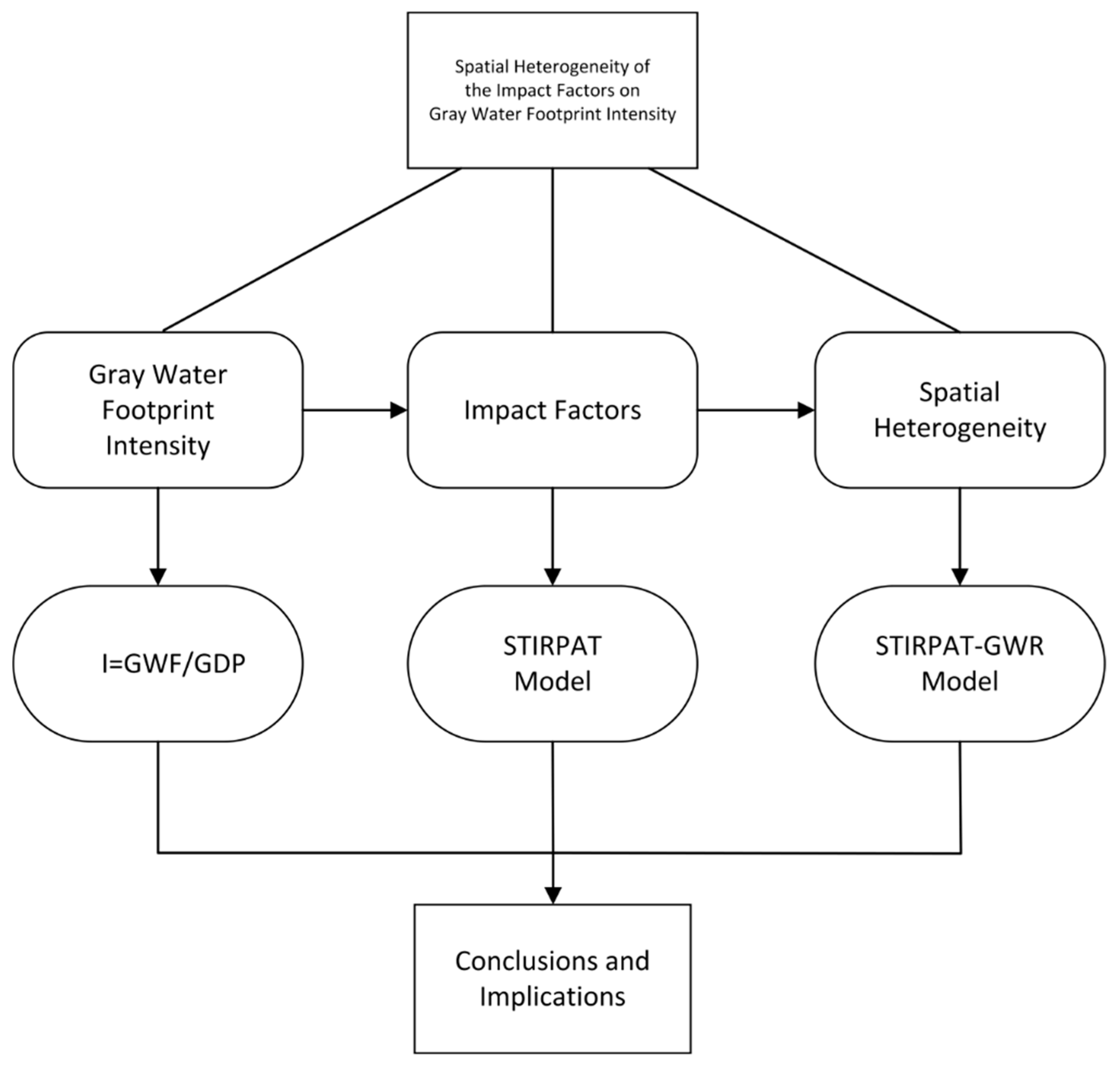
2.1. Research Framework

Gray Water Footprint (GWF) can reflect the status quo of water pollution in the regions and determine the pressure on water resources. The article estimates the gray water footprint of agriculture, industry, life, surface and underground in 31 provinces (autonomous regions) in China and finds out the real pollution in various regions, departments and different water bodies. Gray water footprint intensity as a measure of the extent to which water resources are affected by the economy can reflect the true state of water pollution under regional economic development. From the perspective of spatial correlation, this paper explores the spatial pattern and spatial agglomeration characteristics of gray water footprint in China from 2000 to 2014.Through the construction of STIRPAT model and GWR model, the effects of population size, urbanization rate, output per capita, proportion of tertiary industry, intensity of environmental pollution control and intensity of R&D investment on gray water footprint were analyzed, as well as the spatial heterogeneity of the influencing factors of gray water footprint intensity. At last, it puts forward some countermeasures to control the regional differences and pertinence, allocate regional resources more effectively, promote effective governance of water resources and environment, and ensure the sustainable development of economy, society and ecology. The research framework is seen in Figure 1.

2.2. Gray Water Footprint Calculation Method

2.2.1. Gray Water Footprint of Different Receiving Water

By selecting the pollutant discharge of different pollutants and the corresponding initial concentration and standard pollutant concentration and other data, the amount of freshwater resources required to dilute the pollutants, the gray water footprint, can be calculated. The formula is as follows [27]:

$$GWF=\frac{\lambda \times \alpha \times APPI}{C_{\max }-C_{nat}}$$

(1)

In Formula (1), GWF represents the gray water footprint (m³); λ is the proportion coefficient of pollutants decomposed into different receiving water bodies, and referring to the data of the National Pollution Source Census Bulletin, it was determined that 60.68% of agricultural production pollutants were decomposed into surface water and 39.32% were decomposed into groundwater, that is, the values of λ were 60.68% and 39.32%, respectively; APPI means the pollutant discharge amount (kg); αmeans the leaching rate, and C_max means the water quality of pollutants Standard concentration (kg/m³); C_nat represents the natural initial concentration (kg/m³) of pollutants in receiving water, and C_nat is taken as 0.

2.2.2. Gray Water Footprint on the Surface

The pollutants diluted by surface water mainly include the total COD emissions from agricultural, industrial and domestic parts, the total ammonia nitrogen emissions from industrial and domestic sectors, and the nitrate pollution from agriculture. Therefore, the maximum amount of water required to dilute the three types of pollution is the surface gray water footprint, and the formula is as follows [28]:

$$GW{F}_{sur}=\max \left\{\begin{array}{l}\left(GW{F}_{\mathrm{sur}-\mathrm{agr}\left(\mathrm{COD}\right)}+GW{F}_{sur-ind\left(COD\right)}+GW{F}_{sur-dom\left(COD\right)}\right)\hfill \\ \left(GW{F}_{\mathrm{sur}-\mathrm{ind}\left(\mathrm{NH}-\mathrm{N}\right)}+GW{F}_{\mathrm{sur}-\mathrm{dom}\left(\mathrm{NH}-\mathrm{N}\right)}\right)\hfill \\ GW{F}_{\mathrm{sur}-\mathrm{agr}\left(TN\right)}\hfill \end{array}\right\}$$

(2)

where, GWF_sur-agr(TN) and GWF_sur-agr(COD) are respectively the amount of gray water footprint of planting and aquaculture industries diluted by surface water; GWF_sur-ind(COD) and GWF_{sur-ind(NH-N)} indicate the gray water footprint caused by COD and ammonia emissions from the industrial sector; GWF_sur-dom(COD) and GWF_{sur-dom(NH-N)} indicate the gray water footprint caused by COD and ammonia nitrogen emissions from the domestic sector. The standard COD limit is 20 mg/L; the standard limit for ammonia nitrogen is 1 mg/L; and the standard limit for nitrate is 10 mg/L.

2.2.3. Gray Water Footprint Subsurface

The pollution caused by the agricultural sector is mainly dominated by nitrate pollution and COD pollution from livestock and poultry farming. The formula is [28]:

$$GW{F}_{und}=\max \{GW{F}_{und-agr\left(TN\right)},GW{F}_{und-agr\left(COD\right)}\}$$

(3)

where, GWF_und-agr(TN) and GWF_und-agr(COD) respectively indicate the amount of gray water footprint for planting and aquaculture diluted by groundwater. The standard limit for nitrate (calculated as nitrogen) is 20 mg/L and the standard limit for COD is 3 mg/L.

2.2.4. Gray Water Footprint Total

The sum of the surface gray water footprint and the underground gray water footprint of all provinces in the country is taken as the total gray water footprint of the area. The formula is [28]:

$$GWF=GW{F}_{sur}+GW{F}_{und}$$

(4)

where, GWF indicates gray water footprint total; GWF_sur indicates Gray water footprint on the surface; GWF_und indicates gray water footprint subsurface. The leaching rate of nitrogen fertilizer was 18% and the leaching rate of COD was 22%. According to the data from the National Census Bulletin, 60.68% of agricultural pollutants were decomposed to surface water and 39.32% to groundwater.

2.2.5. Gray Water Footprint Intensity

The gray water footprint intensity representing the amount of fresh water that need dilution of pollutants per unit of output, or the water pollution caused by per output value can reflect the relationship between economy and water pollution. Greater intensity means that the unit of GDP generated more gray water footprint, and as such, diluting pollution will require more fresh water. The formula is [27]:

$$I=\frac{GWF}{GDP}$$

(5)

where, I indicates gray water footprint intensity; unit is m³/10⁴ yuan.

2.3. Spatial Econometrics

There is generally a certain degree of spatial interaction between the economic and geographical behaviors among regions, which is called the spatial effect. Owing to the fact that the spatial data are not completely independent but have some kind of spatial connections, the main research of econometrics is space effect, and the main manifestation of spatial effect is spatial dependence and spatial heterogeneity. Spatial dependence can be defined as the consistency and correlation between observed objects, while spatial heterogeneity can be defined as the nonstationarity and variability of observed objects.

2.3.1. Spatial Autocorrelation

Spatial autocorrelation is a measure of the concentration of values in space, and ties between things closer to each other are stronger than those farther from each other. A positive spatial autocorrelation occurs when a high or low value of a neighboring observation object appears to be agglomerated in space and a negative autocorrelation occurs when adjacent observation objects belong to a heterogeneous nature.

Space Weight Matrix

Spatial weight matrix is the premise of the autocorrelation of the metric space, which is based on the standardization of a binary symmetric adjacency matrix. This spatial weight matrix assumes that all adjacent influences are assumed to be the same while ignoring the non-adjacent spatial correlation. In this paper, the spatial distance weight matrix is used to quantify the spatial location of a region. The elements of the matrix are defined as follows [29]:

$$W_{ij}=\{\begin{array}{ll}0\hfill & i=j\\ 1/d_{ij}\hfill & i\ne j\end{array}$$

(6)

where, d_ij is the distance between the center of gravity of area i and area j.

Global Moran’s I Index

The definition of Global Moran’s I index is [30]:

$$Mora{n}^{\prime }sI=\frac{{{\displaystyle \sum }}_{i=1}^n{{\displaystyle \sum }}_{j\ne i}^n{W}_{ij}{Z}_i{Z}_j}{{\sigma }^2{{\displaystyle \sum }}_{i=1}^n{{\displaystyle \sum }}_{j\ne i}^n{w}_{ij}}$$

(7)

where, $Z_i=\frac{x_i-\overline{x}}{\sigma }$, $\overline{x}=\frac{1}{n}{\displaystyle \sum _{i=1}^n}{x}_i$, ${\sigma }^2=\frac{1}{n}{\displaystyle \sum _{i=1}^n}{\left(x_i-\overline{x}\right)}^2$, n is the number of spatial observations; x_i is the observed value in the spatial position i; Z_i is x_i standardized transformation.

According to the distribution of spatial data, considering the relationship between location and attribute similarity, the expected value and expected variance of the index of Moran’s I can be calculated as follows [30]:

$$E\left(I\right)=-\frac{1}{n-1}$$

(8)

$$Var\left(I\right)=\frac{n\left[(n^2-3n+3)s_1-n{s}_2+3s_0^2\right]-k\left[(n^2-n)s_1-2n{s}_2+6s_0^2\right]}{s_0^2\left(n-1\right)\left(n-2\right)\left(n-3\right)}$$

(9)

where, $s_0={\displaystyle \sum _{i=1}^n}{\displaystyle \sum _{j=1}^n}{W}_{ij}$, $s_1=\frac{1}{2}{\displaystyle \sum _{i=1}^n}{\displaystyle \sum _{j=1}^n}{(W_{ij}+W_{ji})}^2$, $s_2={\displaystyle \sum _{i=1}^n}{({\displaystyle \sum _{j=1}^n}{W}_{ij}+{\displaystyle \sum _{j=1}^n}{W}_{ji})}^2$, $k=\left[{\displaystyle \sum _{i=1}^n}{\left(x_i-\overline{x}\right)}^4\right]/{\left[{\displaystyle \sum _{i=1}^n}{\left(x_i-\overline{x}\right)}^2\right]}^2$.

Z-value statistics for Moran’s I Index [30]:

$$Z=I\frac{I-E\left(I\right)}{\sqrt{Var\left(I\right)}}$$

(10)

Moran’s I Index values range between −1 and 1, where [−1,0) means negative spatial correlation, 0 means spatial uncorrelated, and (0,1] means positive spatial correlation.

Local Moran’s I Index

The definition of Local Moran’s I index is [30]:

$$I_i\left(d\right)=z_i{\displaystyle \sum }_{j\ne i}^n{W}_{ij}{z}_j$$

(11)

where, Z_i and Z_j denote the difference between the measured value and the mean value. When I_i is a positive value, it indicates that the same attribute value in the region is in a state of spatial agglomeration. When I_j is a negative value, it means that different attribute values in the region are presented in the state of space gathering.

2.3.2. Spatial Heterogeneity

Spatial heterogeneity means that the characteristics of the things and phenomena in one spatial location are different from that of the things and phenomena in other locations. This reflects the instability among the economic behaviors of space observation units in economic activities. Things and phenomena are spatially heterogeneous, on the one hand, because various things and phenomena themselves lack a stable spatial structure, and on the other hand, the spatial units themselves differ greatly in all respects. From a statistical point of view, spatial heterogeneity means that the study object is not stable in space. Spatial heterogeneity can be expressed as [31]:

$$y_i=f_i\left(x_i,{\beta }_i,{\epsilon }_i\right)$$

(12)

where, i represents the spatial observation object; f_i represents the functional relationship; y_i represents the dependent variable; x_i represents the independent variable; β_i represents the parameter vector; Ɛ_i represents the error term. The linear relationship is expressed as [31]:

$$y_i=X_i{\beta }_i+{\epsilon }_i$$

(13)

where, X_i represents the vector used to interpret the variable (1 × k).

2.4. STIRPAT Model

In order to reflect the extent of the change of environmental impact when the driving force changes and make hypothesis verification, the classic IPAT model only treats the relationship between environmental impact factors and the dynamics of each area as a linear proportional relationship which cannot reflect the change in environmental impact when the driving force changes, nor can it be verified by assumptions. Therefore, York et al. [32] proposed the STIRPAT model to analyze the non-proportional impact of various factors on environment through statistical regression. General expression is as follows [32]:

$$I=a{P}^b{A}^c{T}^{d}e$$

(14)

where, I is the pressure of the environment; P is the population; A is the margin; T is the technology; a is the constant term of the model; b, c and d are the driving index items of P, A and T respectively; and e is the error term.

In order to analyze the environmental impact of various factors, the formula is logarithmic [32]:

$$\ln \left(I\right)=\ln a+b\ln P+c\ln A+d\ln T+\ln e$$

(15)

where, lnI as dependent variable, lnP, lnA, lnT as independent variable, lna as constant term, lne as error term.

2.5. STIRPAT Geographic Weighted Regression Model

STIRPAT geographic weighted regression model is the combination of STIRPAT model and GWR model, or STIRPAT-GWR model. The spatial position of any one of the study areas is v, and a set of weights at $v$ is denoted as k₁(v), k₂(v), …, k_n(v), representing the effect of observations at each point; k_i(v) corresponds to the observation (y_i, x_i1, x_i2, …, x_ip). The impact of different factors on environmental pollution varies in geospatial space. Geographic weighted regression model can meet the spatial heterogeneity of the influencing factors. STIRPAT-GWR model is:

$$\ln \left(I\right)=a\left(u,v\right)+b\left(u,v\right)\ln P+c\left(u,v\right)\ln A+d\left(u,v\right)\ln T+e$$

(16)

where, (u, v) is the geographical center of the region; a(u, v) is the position function of the constant term and b(u, v), c(u, v), d(u, v)are positional functions of independent variable coefficients.

2.6. Ridge Regression Method

The Ridge Regression method, proposed by Hoed and Kennard in 1970, is an effective way to reduce the variance of parameter estimates at the expense of introducing errors. The standard ridge regression equation can be obtained by using SPSS statistical software [24]:

$$Y=a_1{X}_1+a_2{X}_2+\dots +a_k{X}_k$$

(17)

where, a_k is the standard regression coefficient of the kth argument; Y is the dependent variable, and X_k is the kth independent variable. Ridge regression equation can be obtained by calculating the standard Ridge regression equation [24]:

$$Y=b_1(X_1)+b_2\left(X_2\right)+\dots +b_k(X_k)+b_0$$

(18)

where, all the obtained independent variable coefficients represent the elastic coefficients of the respective variables in the STIRPAT model, and b₀ represents the constant term.

2.7. Data Sources

The data of nitrogenous fertilizer application, gross domestic product, or GDP, total population, urbanization rate, per capita output value and proportion of tertiary industry in agricultural departments of all provinces and cities all come from China Statistical Yearbook (2001–2015) and The Statistical Yearbook of all provinces (2001–2015). Data on COD emissions from the agricultural sector and COD and ammonia nitrogen emissions from the industrial and domestic sectors are taken from China Statistical Yearbook on Environment (2001–2015) and China Yearbook of Environmental Sciences (2001–2015). Relevant data on intensity of environmental pollution control come from China Environmental Yearbook (2001–2015). The relevant data of R&D funding intensity are from National Science and Technology Progress Statistics Monitoring Report.

3. Results and Discussions

3.1. Chinese Gray Water Footprint Intensity Results and Analysis

It is calculated that overall gray water footprint intensity of all provinces in the country shows a downward trend during 2000 and 2014 (Figure 1). Among them, Ningxia, Gansu, Guangxi, Jilin and other regions presented the most obvious decline. The intensity of the agricultural gray water footprint in Ningxia declined most dramatically, from 4148.52 m³/10⁴ in 2000 to 939.45 m³/10⁴ in 2014. Furthermore, its industrial gray water footprint intensity was 7548.9 m³/10⁴ in 2000.Although the gray water footprint in these areas declined dramatically, their average gray water footprint intensity were the highest, resulting in the most serious water pollution caused by inefficient economic development. The gray water footprints of the four regions of Fujian, Shanghai, Jiangsu and Tianjin are the lowest, and the intensity of the initial gray water footprint is small in 15 years. However, the intensity of agricultural gray water footprint in Tibet declined from 657.33 m³/10⁴ in 2000 to 456.91 m³/10⁴ in 2014. The economic development has had little impact on water pollution.

With their special geographical condition and limited developed regions and agricultural scale, Xizang, Hainan and other regions have relatively low output value and gray water footprint, and high efficiency of economic development and water resources utilization. As can be seen from Figure 2, the gray water footprint intensity in these regions such as Qinghai, Jiangsu, Guangdong and Heilongjiang are generally low because the initial value of intensity is small and declines every year. Although the decline rate is small during the study period, in general, the influence of economic factors on water pollution is not significant, and water resources utilization efficiency under economic development is the highest.

3.2. Spatial Correlation Analysis of Chinese Gray Water Footprint Intensity

3.2.1. Global Spatial Autocorrelation Analysis

According to the data of Chinese gray water footprint intensity from 2000 to 2014, the global Moran’s I index of gray water footprint intensity of each year is obtained by using the global spatial auto-correlation analysis model, as shown in

Table 1. The global spatial autocorrelation index of the economy and water pollution in China.

Year	Moran’s I	$\mathit{Z}\left(\mathit{I}\right)$	$\mathit{P}$	Year	Moran’s I	$\mathit{Z}\left(\mathit{I}\right)$	$\mathit{P}$
2000	0.0236	1.6618	0.0224	2008	0.0212	2.0669	0.0060
2001	0.0306	1.6133	0.0200	2009	0.0356	2.5835	0.0020
2002	0.0114	1.5532	0.0280	2010	0.0367	2.7755	0.0020
2003	0.0186	1.0788	0.0620	2011	0.0441	2.5631	0.0020
2004	0.1967	1.2868	0.0300	2012	0.0442	2.2645	0.0020
2005	0.1887	1.7308	0.0420	2013	0.0404	2.8972	0.0010
2006	0.0096	2.8834	0.0080	2014	0.0418	2.0143	0.0010
2007	0.0162	2.7327	0.0100

. The P statistic for each year shows that the data passed the significance test of the model. Since the beginning of 2000, the Moran’s I index has fluctuated, but overall, the Moran’s I index showed an upward trend. The results show that the intensity of gray water footprint in China has a global autocorrelation in 15 years, and the autocorrelation is continuously increasing.

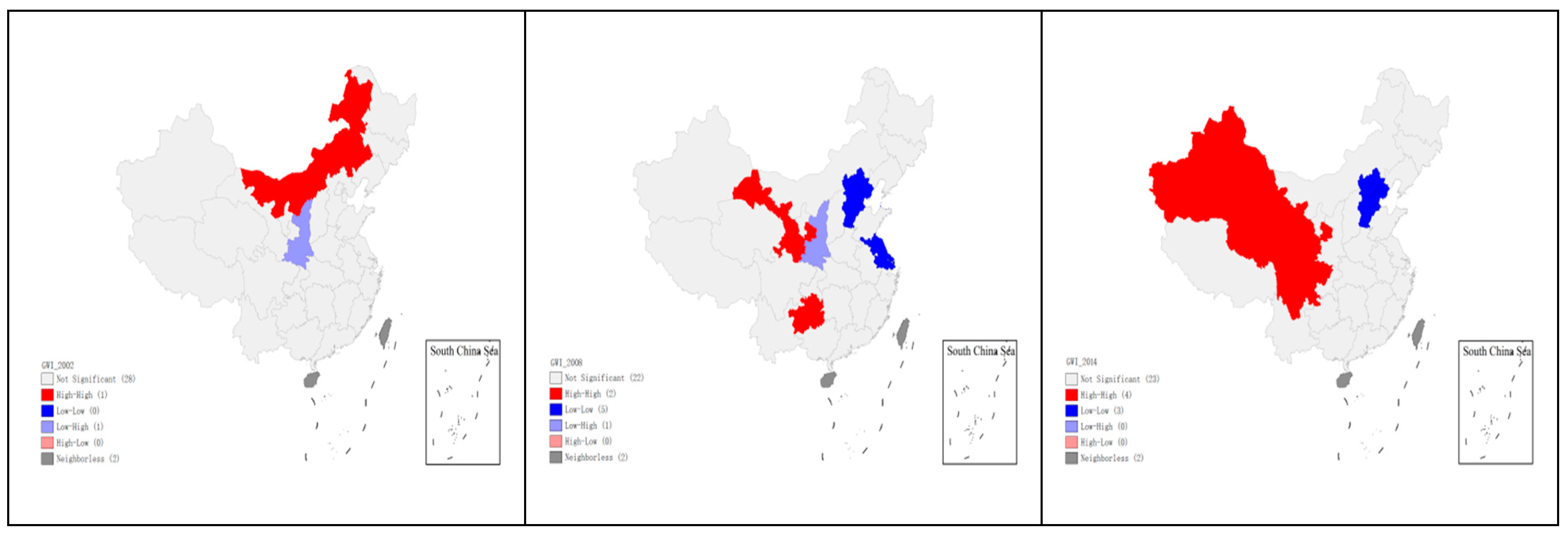
3.2.2. Local Spatial Autocorrelation Analysis

According to the aggregated maps of the gray water footprint intensity of provinces in China in 2002, 2008 and 2014, there is a clear spatial clustering characteristic among the gray water footprint intensities of the regions and mainly shows two types of aggregation, that is, High–High (HH) agglomeration and Low–Low (LL) agglomeration, as shown in Figure 3. —HH indicates that this area and its neighboring areas are both high-value areas, while LL indicates that this area and its neighboring areas are both low-value areas.

The HH agglomeration area is located in the western part of China. These areas feature high gray water footprint intensity and high gray water footprint intensity in their adjacent areas, which indicates that the economic development in these areas has a greater impact on water pollution, resulting in more gray water footprint, slower speed of economic development compared with the increase rate of gray water footprint and the inefficiency of economic development, which has a greater negative impact on neighboring areas.

The LL agglomeration is mainly concentrated in Northeast and North China, including Jilin, Liaoning, Hebei and Tianjin. The intensity of the gray water footprint in these provinces is relatively small and the GDP of these regions is relatively high. Owing to reasonable industrial structure and improvement of sewage technology, the emissions of pollutants in these regions are low and the impact of economic development on water pollution is little. Furthermore, these provinces can form a low-lying agglomeration, setting an example in driving the positive impact on the development of the surrounding areas, and can continue to promote the sustainable development of water resources in our country.

3.3. Spatial Heterogeneity of the Impact Factors on Gray Water Footprint Intensity in China

3.3.1. Selection of Influencing Factors

The gray water footprint intensity is selected as a dependent variable to refer to environmental stress indicators. The total population, urbanization rate, the proportion of working population are selected as the indicators for population size. Gross domestic product, output value per capita, consumption level of residents, proportion of agriculture, proportion of secondary industry, contribution rate of secondary industry and proportion of tertiary industry are chosen as the indicators for affluence. Agricultural gray water footprint intensity, industrial gray water footprint intensity, total environmental pollution control, environmental pollution control intensity, R&D investment and R&D investment intensity are selected as the indicators for technology. The least square method was used to select the 16 influencing factors and remove the factors producing the same effect. Finally, the total population, urbanization rate, output per capita, proportion of tertiary industry, intensity of environmental pollution control and intensity of R&D investment are selected respectively as the indicators for population size, affluence and technology.

The study selects the annual population as an indicator for population size; urbanization rate, or the ratio of urban population to the total population as an indicator of social development; and per capita output as an indicator for the level of economic development. For any region, a large amount of waste will be produced during its process of economic development, which will in turn affect the utilization of water resources and lead to the deterioration of the water environment. The proportion of tertiary industry is an indicator of industrial structure. The intensity of environmental pollution control refers to the ratio of environmental pollution control investment to GDP. Furthermore, R&D investment intensity is the ratio of the annual expenditure on research and development to the current GDP. The increase in the total population increases the resource consumption, pollutant discharge, and gray water footprint, which directly affects the intensity of the gray water footprint. Taking the proportion of the urban population in the total population as an indicator of the state of social development, and when the urbanization rate increases, resource production and consumption, and gray water footprint in the corresponding areas increase. The per capita output value can reflect the degree of wealth of the region. The higher the per capita output value, the higher the living standard and the greater the living demand, and the increase in resource consumption will worsen water pollution. The change in the proportion of the tertiary industry will affect the type of pollutant discharge, which will also lead to differences in the amount of water that dilutes the pollution. The intensity of environmental pollution treatment is used as an indicator to measure the efforts of various regions to invest in the treatment of gray water, to analyze the relationship between the proportion of investment in different environmental pollution and the change in the intensity of gray water footprint. The intensity of R&D input is the ratio of annual national research and development expenditure to the GDP of that year. The intensity of gray water footprint can be reduced by improving technology and innovative production methods to change the industrial structure.

3.3.2. Establish STIRPAT Model

The six indicators of total population, urbanization rate, output value per capita, proportion of tertiary industry, intensity of environmental pollution control and R&D investment intensity are introduced into the model. The expanded STIRPAT model is expressed as [32]:

$$\ln I=lna+b_p\ln P_p+b_c\ln P_c+c_g\ln A_g+c_t\ln A_t+d_e\ln T_e+d_{r}ln{T}_r+\ln e$$

(19)

where, I is the environmental pressure of water pollution, expressed in gray water footprint intensity and the unit is m³/10⁴ yuan; P_p is the total population and the unit is ten thousand; P_c is the urbanization rate whose the unit is expressed in%; A_g is the per capita output value whose unit is the yuan; A_t is the industrial structure, that is, the proportion of the tertiary industry and the unit expressed in%; T_e is the intensity of environmental pollution control, expressed in%; T_r is R&D investment intensity, expressed in%; b_p, b_c, c_g, c_p, d_e, d_r are the correlation coefficients respectively.

3.3.3. Least Squares Regression Results

Based on the data in the table, combined with Equation (19), a multivariate linear regression was performed using the least squares method and its coefficient of determination, significance, and VIF were obtained by using SPSS software. Fitting reports from the China-related STIRPAT model 2000–2014 show the results of multiple linear regression. As shown in

Table 2. Least squares regression results of model.

R2	Adjusted R2	F	Significance
0.987	0.977	99.877	0.000

, the F value is 99.877; the Sig is 0.000; the height is significant; R² is 0.987; the adjusted R² is 0.977; the fitting effect is good, and the dependent variable and the independent variable are strongly correlated. The indicator selection meets the requirements and regression analysis makes sense.

Next, the coefficient estimation of each indicator of the model is carried out, and the collinearity test is carried out to obtain the Variance Inflation Factor (VIF) values of the indicators of population, urbanization rate, per capita output value and R&D expenditure intensity, which are respectively 1359.067, 1922.411, 171.615, 124.797, far greater than 10. Therefore, the multiple collinearity among these data can be found. Therefore, the least squares method is not suitable for STIRPAT model analysis. In order to solve the problem of collinearity, it is necessary to use ridge regression analysis.

3.3.4. Ridge Regression Fitting Results

A fitting report can be obtained and analyzed through ridge regression fitting. The coefficient K in the ridge regression was taken in the interval (0,1). After fitting the STIRPAT model, the regression coefficients of the independent variables tended to be stable when K = 0.05. The coefficient of determination R² was 0.972 and its good fitness passed the test of significance. As shown in

Table 3. The ridge regression results when k = 0.05.

R2	Adjusted R2	F	Significance
0.972	0.951	46.248	0.000

, the test values of the independent variables are both greater than 2 and the p values are less than 0.05, which shows that the linear correlation between the dependent variable and the independent variable is significant, and the regression equation has statistical significance.

Therefore, the STIRPAT model is [33]:

$$\ln I=61.654-3.844\ln P_p-0.728\ln P_c-0.339\ln A_g-0.97\ln A_t-0.547\ln T_e-0.102ln{T}_r$$

The Ridge regression equation of the standardized STIRPAT model is [33]:

$$\ln \overline{I}=-0.163\ln \overline{P_p}-0.171\ln \overline{P_c}-0.37\ln {\overline{A}}_g-0.087\ln {\overline{A}}_t-0.165\ln {\overline{T}}_e-0.048ln{\overline{T}}_r$$

3.3.5. Analysis of Model Test Results

The absolute value of the standard regression coefficient can measure the relative impact of the corresponding influencing factors on the environment. The regression coefficient indicates the elasticity of driving force (influencing factor) to environmental pressure (gray water footprint intensity), which refers to the percentage change of gray water footprint resulting from the 1% change in any one of indicators of the total population, urbanization rate, output value per capita, the tertiary industry share, environmental pollution control intensity, R&D investment intensity. Furthermore, this effect can be either positive or negative.

As shown in

Table 4. The ridge regression results of various of the model.

	Non-Standard Coefficient	Standardized Coefficient	T Statistic	Significance
Constant	61.6539		4.776	0.001
The total population	−3.844	−0.163	−3.261	0.01
Urbanization rate	0.728	0.171	−3.894	0.004
Per capita output value	−0.339	−0.370	−4.281	0.002
The tertiary industry share	−0.970	−0.087	−3.801	0.004
Environmental pollution control intensity	−0.547	−0.165	−2.936	0.02
R&D investment intensity	−0.102	−0.048	−2.547	0.032

, ridge regression results of the model show that among the six influencing factors of gray water footprint intensity, only the urbanization rate is positively correlated with the gray water footprint intensity, and the other five are negatively correlated with the gray water footprint intensity. According to the impact, the order is as follows: output value per capita (−0.370), urbanization rate (0.171), environmental pollution control intensity (−0.165), the total population (−0.163), the tertiary industry share (−0.087), R&D investment intensity (−0.048).

3.3.6. Analysis of Impact Factors

(1) The total population

From 2000 to 2014, the total population of the country increased from 1267.43 million to 1.36782 billion. The larger the population is, the more direct gray water footprints are. However, people are also creating economic output while generating the gray water footprint. This mutual offsetting effect makes it difficult to measure the impact of population factors on the gray water footprint intensity. By constructing STIRPAT model, the data of the impact of China’s total population on the gray water footprint intensity from 2000 to 2014 can be drawn. The results show that the total population has a greater impact on the gray water footprint intensity and has the highest elasticity. Without changing other factors, an increase in the national population will promote a reduction in the intensity of the gray water footprint.

(2) Urbanization rate

In the STIRPAT model, the urbanization rate mainly reflects the production and consumption behavior of residents as a result of the changes in population urban-rural structure and the impact of changes in consumption patterns on gray water footprint and economic development [34]. From 2000 to 2014, the urbanization rate in China increased from 36.22 to 54.77%, an increase of 18.55%. The results of the model data show that the urbanization rate has a positive impact on the gray water footprint intensity, which means that for every 1% increase in the urbanization rate, the gray water footprint intensity will increase by 0.728% accordingly. It shows that the economic development brought by the improvement of urbanization level at this stage cannot make up for the pollution damage caused by urbanization.

(3) Per capita output value

In spite of the continuous improvement of economic development, the extent of the destruction of the environment is also increasing. However, after the economy reaches a certain level, the pollution of the environment will be reduced again. The per capita output value at the 5% significance level had a negative impact on the improvement of water footprint in China, with the greatest impact. For every 1% increase in per capita output, the gray water footprint will decrease by 0.796% accordingly. This shows that the larger the per capita output value, the lower the gray water footprint in the region, and higher output value is conducive to reducing the intensity of the gray water footprint.

(4) The tertiary industry share

During the period of 2000–2014, the tertiary industry in our country has been developing rapidly, and its proportion has been increasing year by year, from 39.8% in 2000 to 47.8% in 2014. The development of the tertiary industry economy has made an important contribution to the growth of the national economy. Through the analysis of influencing factors, there is a negative correlation between the proportion of tertiary industry and the intensity of gray water footprint. Furthermore, for every 1% increase in the proportion of the tertiary industry, the gray water footprint will be reduced by 0.970% accordingly.

(5) Environmental pollution control intensity

The intensity of environmental pollution control also has a positive effect on the increase of the footprint of gray water, that is, for every 1% increase in the intensity of environmental pollution control, the gray water footprint intensity will be reduced by 0.547% accordingly. Investment in environmental pollution refers to the investment directly used in pollution control facilities. Increasing the investment in environmental protection in the region will reduce the amount of gray water footprint in the region and reduce the consumption of gray water footprint to a certain extent, thereby reducing the intensity of gray water footprint.

(6) R&D investment intensity

R&D investment intensity refers to the intensity of investment in research and development, also playing an opposite effect on the increase in the intensity of gray water footprint. For every 1% increase in R&D investment intensity, the gray water footprint intensity will decrease by −0.102% correspondingly. The region with more developed science and technology will boast greater ability and tension to create economic output. The region with more advanced science and technology will achieve greater improvements in the corresponding secondary and tertiary industry modes of production and operation and water-saving technologies. As a result, the water consumption of production will be reduced; the discharge rate of industrial wastewater will reach the standard, and the consumption of gray water footprint will be reduced.

3.4. STIRPAT-GWR Model Test

Capital cities are the political, economic and cultural centers of provinces, and have a major impact on the province and its surrounding areas [35]. Therefore, this study chooses the latitude and longitude of the capital cities as geographical coordinates, fixed Gaussian function as the weight function, cross-validation method to determine the bandwidth, and the AICc bandwidth method of “adaptive” kernel function for local estimation. Furthermore, using GWR4.0 software, on the basis of strict parameter test, the corresponding regression calculation is carried out to explore the spatial heterogeneity of influencing factors of gray water footprint intensity. From

Table 5. The test results of the GWR model from 2000 to 2014.

	Bandwidth	AICc	R2	F
2000	2.609	30.832	0.992	1.906
2001	2.682	22.607	0.997	3.664
2002	2.655	30.521	0.994	2.059
2003	2.698	30.166	0.997	4.078
2004	2.780	25.031	0.997	2.889
2005	2.731	36.998	0.995	2.012
2006	2.569	26.617	0.997	3.359
2007	2.596	16.715	0.998	4.021
2008	2.581	14.354	0.997	2.933
2009	2.568	13.005	0.997	1.597
2010	2.650	8.622	0.998	2.380
2011	2.638	16.286	0.998	2.881
2012	2.631	2.188	0.998	2.548
2013	2.672	3.036	0.997	1.851
2014	2.629	2.750	0.995	1.358

, we can see that the goodness of fit of GWR model between 2000 and 2014 is higher than 0.992, showing that the fitting result is better and the data test result is reasonable.

3.5. Spatial Heterogeneity of the Impact Factors

GWR can characterize the spatial heterogeneity of the influencing factors of the gray water footprint intensity in each province as the geographic distance changes. By constructing the GWR model, the regression coefficients of influencing factors of gray water footprint intensity in all provinces from 2000 to 2014 are obtained. We made Figure 4, Figure 5, Figure 6, Figure 7, Figure 8 and Figure 9 using ArcGIS tool. Figure 4, Figure 5, Figure 6, Figure 7, Figure 8 and Figure 9 shows the spatial heterogeneity of the six factors affecting the gray water footprint intensity, where the years 2002, 2008 and 2014 are chosen as representative years.

3.5.1. Spatial Heterogeneity of the Impact of Total Population on Gray Water Footprint Intensity

Between 2000 and 2014, there was an either positive or negative correlation between the total population and the gray water footprint intensity in all regions. The larger the population, the more consumption it consumes, and the greater its gray water footprint will be. However, while creating pollution, people are also creating economic output that offset their effects. In Northeast China and East China, the total population and the gray water footprint intensity basically showed a positive correlation, and the increase of the total population led to the increase of the intensity of the gray water footprint. The relationship between population and gray water footprint intensity in North China and South China experienced a change from negative to positive, and then from positive to negative and population growth stimulated less intensity of gray water footprint, which brought a positive impact. However, the increase in the total population of cities like Tibet, Gansu, Shaanxi whose intervals of the regression coefficients are (−0.958, 0.108), (−0,381, −0.006), (−0.452, 0.018), has always contributed to the reduction in the intensity of gray water footprint. Overall, by 2008, the population in most regions had a positive impact on the intensity of gray water footprint. By 2014, the population in most regions had a greater negative impact on the intensity of gray water footprint.

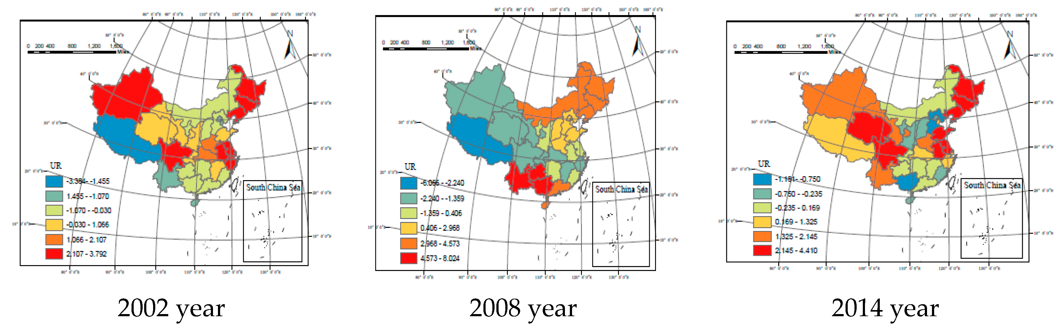
3.5.2. Spatial Heterogeneity of the Impact of Urbanization Rate on Gray Water Footprint Intensity

As can be seen from Figure 5, the regression coefficient of urbanization rate in most regions of the country by 2014 is positive, which means that there is a positive correlation between urbanization rate and gray water footprint intensity. Furthermore, the influence of urbanization rate on the gray water footprint intensity gradually increases, and the increase of urbanization rate also gradually increases the gray water footprint intensity. This shows that the increase of urbanization promotes economic development of the city, but meanwhile, it also produces more consumption and pollution and has a negative impact on the intensity of the gray water footprint. From the perspective of space and time, from 2000 to 2014, the change of the regression coefficient value in the western and eastern regions of China is the largest, and the positive correlation has gradually increased. The relationship between the urbanization rate and the intensity of gray water footprint in the Western region, including most of the cities in the northwest and southwest regions, has changed to a positive correlation from a negative one, while in the eastern region, especially in the northeast, there has always been a positive correlation.

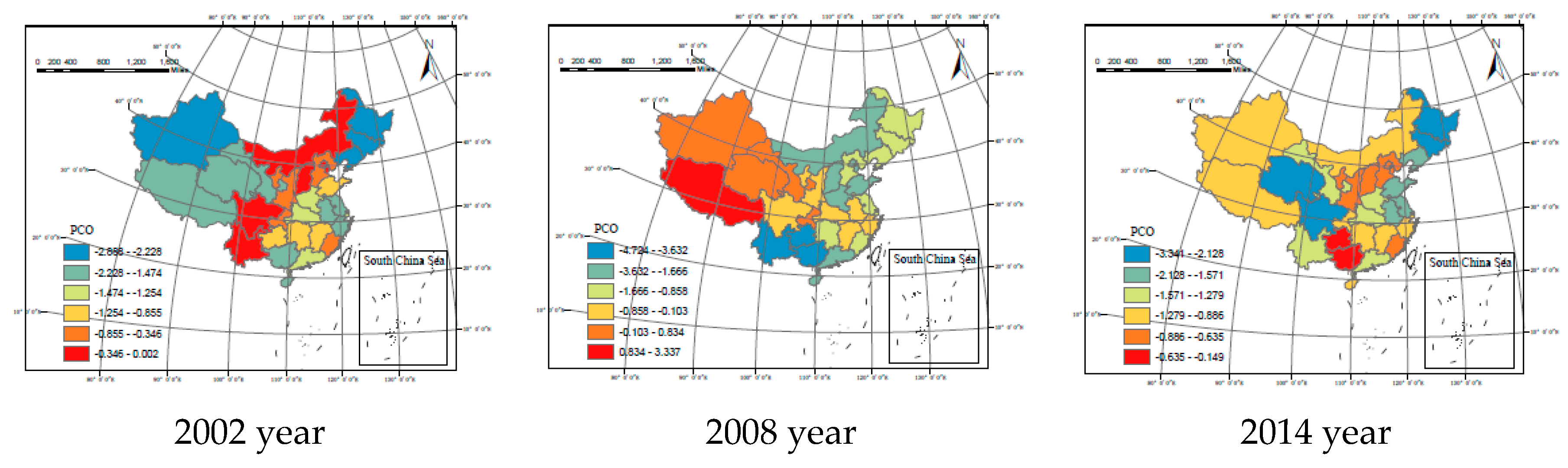
3.5.3. Spatial Heterogeneity of the Impact of Output Value per Capita on Gray Water Footprint Intensity

GWR model analysis shows that the regression coefficient of per capita output from 2000 to 2014 is negative in all regions, showing a negative correlation, indicating that the economic growth can promote the reduction of gray water footprint intensity. As shown in Figure 6, the coefficient range from −2.8885 to −0.0006 in 2002; the coefficient range from −4.7242 to −0.8943 in 2008, and the coefficient range for 2014 is −3.3413 to −0.1495, indicating that the per capita output is not only negatively correlated with gray water footprint intensity, but also has significant spatial changes of the impact.

In general, since 2000, the value of the regression coefficient of per-unit output value of various provinces and cities has risen slowly and began to decline slowly after 2008, with the change range decreasing by 2012, but the per-capita output value still has a strong negative correlation with other regions. Northwest and Southwest China have the largest changes, and per capita output produces deep impact on the gray water footprint. For Northeast China, namely, Heilongjiang, Jilin and Liaoning, economic growth has the greatest and deepest impact on gray water footprint intensity, and the per capita output value can actively promote the reduction of gray water footprint intensity. In North China and East China, the coefficient of per capita output value fluctuates slightly but has a large effect. In 2014, the coefficient values are basically greater than −0.64.

3.5.4. Spatial Heterogeneity of the Impact of Tertiary Industry Share on Gray Water Footprint Intensity

As it can be seen from Figure 7, the regional spatial correlation of the regression coefficient of the proportion of the tertiary industry is obvious. In 2002, the proportion of tertiary industry in China’s northwestern and southeastern coastal areas was positively correlated with the intensity of gray water footprint, but the positive impact was small. However, by 2008 and again in 2014, the regression coefficient in most regions turned negative, which means that the larger tertiary industry leads to smaller gray water intensity and greater impact. By 2014, on the whole, the degree of negative influence declines from northeast to southwest, while the regions with large negative correlation include Northeast, North China and most of East China. The industrial structure changes in these areas are more likely to affect the gray water footprint intensity. Therefore, in the development of these regions, more attention should be paid to the adjustment of industrial structure. The change from positive to negative and the increase of the absolute value of the negative correlation coefficient all indicate that the continuous adjustment of industrial structure is an important factor to promote the reduction of gray water footprint intensity and the degree of influence is gradually increasing. During the period, the absolute values of the correlation coefficients of the provinces of Yunnan (−9.507, −0.164), Guangxi (−9.567, −0.318) and Hainan (−5.443, −0.452) changed most obviously, which indicates that the continuous adjustment of the industrial structure is an important factor to promote the reduction of the intensity of the gray water footprint.

3.5.5. Spatial Heterogeneity of the Impact of Environmental Pollution Control Intensity on Gray Water Footprint Intensity

Overall, the absolute value of the regression coefficient of the strength of regional environmental pollution control is significantly less than the regression coefficient of other factors, indicating that the strength of environmental pollution control has a weaker impact on gray water footprint intensity, compared with other factors. In 2014, the impact decreased from the south to the north. As can be seen from Figure 8, from 2000 to 2014, the regression coefficient value of environmental pollution intensity in most areas changed from positive to negative, or from positive correlation to negative one, with the largest change in the northwest and southwest.

However, overall, before 2008, the intensity of environmental pollution control in Western China would not bring about a decrease in the intensity of gray water footprint. By 2014, the impact of environmental pollution control intensity on the gray water footprint intensity would be relatively weak. This is related with the level of economic development and the geographical environment in the western region. The intensity of environmental pollution control in the southeastern coastal areas of China has the greatest stimulating effect on the footprint intensity of gray water. Therefore, it is necessary to increase investment in environmental pollution control in the northeastern coastal areas.

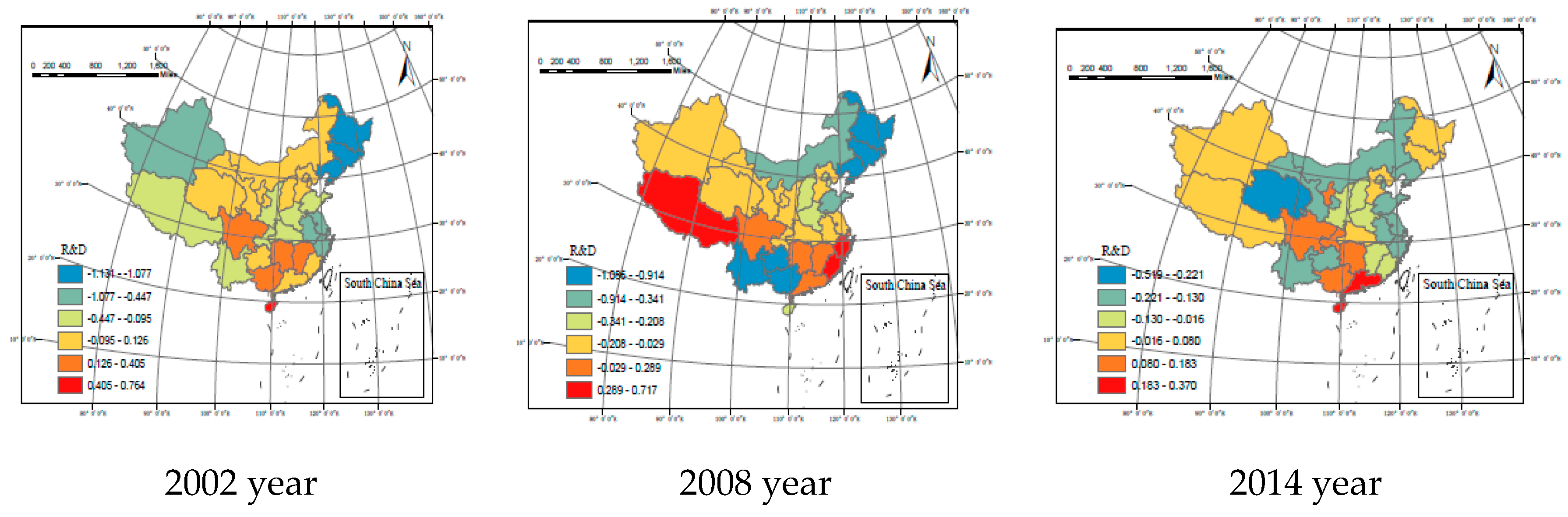
3.5.6. Spatial Heterogeneity of the Impact of R&D Investment Intensity on Gray Water Footprint Intensity

Overall, increasing R&D spending in most parts of the country by 2014 can drive a reduction in the intensity of gray water footprint. Furthermore, there is a small difference in the regression coefficient values of R&D investment intensity among regions, which means that there is little difference in the degree of impact. From 2000 to 2014, the intensity of R&D expenditure in the northern part of China, including Northeast, Northwest and Northern China, has been negatively correlated with the gray water footprint intensity. This shows that the increasing investment in research funding can actively promote the continuous reduction of gray water footprint.

4. Conclusions and Implications

The study found that gray water footprint intensity in all provinces in China has obvious global and local spatial autocorrelation. Northeast and North China feature Low-Low agglomeration and promote the common development in this region and the surrounding areas. From a nationwide perspective, among the six influencing factors of gray water footprint intensity, only the urbanization rate is positively correlated with the gray water footprint intensity, and the other five are negatively correlated with the gray water footprint intensity. This shows that the acceleration of urbanization, accompanied by the energy consumption in life and the growth of various needs, has led to an increase in the intensity of the gray water footprint. The development of urbanization is also conducive to improving the efficiency of resource use and pollution control effects, thus helping to alleviate the pressure on the ecological environment. However, when the overall urban development level is relatively low, population growth, improvement of living standards and economic development will mean more possession and depletion of natural resources, leading to a large amount of pollution in development. It shows that the economic development brought by the improvement of urbanization at this stage cannot make up for the pollution damage caused by urbanization.

According to the spatial heterogeneity analysis of regional influencing factors, it is found that there is a positive correlation between the total population and the intensity of gray water footprint in most parts of Northeast China and East China. Most other regions showed a basic negative correlation. This shows that under the premise of an increase in population, our country must pay attention to the improvement of population quality, which plays an increasingly important role in economic growth and social development. The urbanization rate in most areas shows a strong positive correlation with the gray water footprint, which means that the urbanization rate cannot make up for the damage to water resources due to its economic development. The per capita output value in all regions of China shows a negative correlation with the gray water footprint strength, and the impact is greater. Although the level of economic development is constantly increasing and the degree of environmental destruction is also increasing, the level of environmental pollution will be reduced after the economy reaches a certain level. Therefore, the most direct and effective way for all regions to effectively reduce the gray water footprint is to develop their economy and expand their total economic output. Furthermore, the rate of output growth in the region is greater than the rate of increase in the consumption of gray water due to higher consumption levels.

The impact of the proportion of the tertiary industry on the negative correlation of gray water footprint intensity increases from Southwest to Northeast China. Furthermore, there exists the greatest negative correlation in Northeast, North and East China, which means that the optimization and upgrading of industrial structure is an important way to reduce the gray water footprint. Generally speaking, the impact of environmental pollution control intensity on the intensity of gray water footprint in most parts of China is relatively weak. However, for the sustainable development of the region, although environmental pollution control can produce few economic benefits, in the face of the increasingly serious water pollution in our country, all regions should attach importance to the investment in pollution control. From the perspective of development trend, the negative impact of the intensity of R&D spending on China’s gray water footprint intensity becomes stronger, so the scientific research investment becomes more and more important. The improvement of the quality of the population is required for modern production and lifestyles. People should constantly use their own knowledge and skills to meet their own needs and cultivate their own environmental awareness, which can indirectly protect the resources and environment.

References

1. Shahpouri, A.; Biabi, H.; Abolhassani, L. Economic development and environmental quality: The environmental Kuznets curve for water pollution. J. Appl. Sci. Environ. Manag. 2016, 20, 161–169. [Google Scholar] [CrossRef] [Green Version]
2. Cazcarro, I.; Duarte, R.; Sanchez Choliz, J. Downscaling the gray water footprints of production and consumption. J. Clean. Prod. 2016, 132, 171–183. [Google Scholar] [CrossRef] [Green Version]
3. Hoekstra, A.Y.; Mekonnen, M.M. The water footprint of humanity. Proc. Natl. Acad. Sci. USA 2011, 109, 3232–3237. [Google Scholar] [CrossRef] [PubMed] [Green Version]
4. Zhang, F.; Zhang, Q.; Li, F.; Fu, H.Y.; Yang, X.H. The spatial correlation pattern of water footprint intensity and its driving factors in China. J. Nat. Resour. 2019, 34, 934–944. [Google Scholar]
5. Anselin, L. Spatial Econometrics: Methods and Models; Kluwer Academic: Boston, MA, USA, 1988. [Google Scholar]
6. Hoekstra, A.Y.; Chapagain, A.K. Water footprints of nations: Water use by people as a function of their consumption pattern. Water Resour. Manag. 2007, 21, 35–48. [Google Scholar] [CrossRef]
7. Chapagain, A.K.; Hoekstra, A.Y. The blue, green and gray water footprint of rice from production and consumption perspectives. Ecol. Econ. 2011, 70, 749–758. [Google Scholar] [CrossRef]
8. Chapagain, A.K.; Hoekstra, A.Y.; Savenije, H.H. Water saving through international trade of agricultural products. Hydrol. Earth Syst. Sci. 2006, 10, 455–468. [Google Scholar] [CrossRef] [Green Version]
9. Ruini, L.; Marino, M.; Pignatelli, S.; Laio, F.; Ridolfi, L. Water footprint of a large-sized food company: The case of Barilla pasta production. Water Resour. Ind. 2013, 1, 7–24. [Google Scholar] [CrossRef] [Green Version]
10. Ercin, A.E.; Aldaya, M.M.; Hoekstra, A.Y. Corporate water footprint accounting and impact assessment: The case of the water footprint a sugar-containing carbonated beverage. Water Resour. Manag. 2011, 25, 721–741. [Google Scholar] [CrossRef]
11. Mekonnen, M.M.; Hoekstra, A.Y. National water footprint accounts: The green, blue and gray water footprint of production and consumption. In Value of Water Research Report Series; UNESCO-IHE: Delft, The Netherlands, 2011; pp. 17–22. [Google Scholar]
12. Mekonnen, M.M.; Lutter, S.; Martinez, A. Anthropogenic nitrogen and phosphorus emissions and related gray water footprints caused by EU-27’s crop production and consumption. Water 2016, 8, 30. [Google Scholar] [CrossRef] [Green Version]
13. Vanham, D.; Bidoglio, G. The water footprint of agricultural products in European river basins. Environ. Res. Lett. 2014, 9, 64–70. [Google Scholar] [CrossRef]
14. Brueck, H.; Lammel, J. Impact of fertilizer N application on the gray water footprint of winter wheat in a NW-European temperate climate. Water 2016, 8, 356. [Google Scholar] [CrossRef]
15. Huang, W.X.; Yan, B.; Ji, J.M. A review of researches on the gray water footprint. Environ. Eng. 2017, 35, 149–153. [Google Scholar]
16. Jorrat, M.D.; Araujo, P.Z.; Mele, F.D. Sugarcane water footprint in the province of Tucuman, Argentina. Comparison between different management practices. J. Clean. Prod. 2018, 18, 521–529. [Google Scholar]
17. Muyibi, S.A.; Ambali, A.R.; Eissa, G.S. The impact of economic development on water pollution: Trends and policy actions in Malaysia. Water Resour. Manag. 2008, 22, 485–508. [Google Scholar] [CrossRef]
18. Hoekstra, A.Y.; Chapagain, A.K. Globalization of Water: Sharing the Planet’s Freshwater Resources; Black-Well Publishing: Oxford, UK, 2008. [Google Scholar]
19. Ercin, A.E.; Hoekstra, A.Y. Water footprint scenarios for 2050: A global analysis. Environ. Int. 2014, 64, 71–82. [Google Scholar] [CrossRef]
20. Durán, O.; Durán, P. Activity based costing for wastewater treatment and reuse under uncertainty: A fuzzy approach. Sustainability 2018, 10, 2260. [Google Scholar] [CrossRef] [Green Version]
21. Zhang, P.; Huang, G.; An, C.; Fu, H.; Gao, P.; Yao, Y.; Chen, X. An integrated gravity-driven ecological bed for wastewater treatment in subtropical regions: Process design, performance analysis, and greenhouse gas emissions assessment. J. Clean. Prod. 2019, 212, 1143–1153. [Google Scholar] [CrossRef]
22. Knight, J.; Ingram, D.L.; Hall, C.R. Understanding irrigation water applied, consumptive water use, and water footprint using case studies for container nursery production and greenhouse crops. Horttechnology 2019, 29, 693–699. [Google Scholar] [CrossRef]
23. Li, H.Y.; Wang, Y.F.; Qin, L.J. Effects of different slopes and fertilizer types on the grey water footprint of maize production in the black soil region of China. J. Clean. Prod. 2020, 246, 119077. [Google Scholar] [CrossRef]
24. Larsen, T.A.; Hoffmann, S.; Lüthi, C.; Truffer, B.; Maurer, M. Emerging solutions to the water challenges of an urbanizing world. Science 2016, 352, 928–933. [Google Scholar] [CrossRef] [PubMed]
25. Dinda, S. Environmental Kuznets curve hypothesis: A Survey. Ecol. Econ. 2004, 49, 431–455. [Google Scholar] [CrossRef] [Green Version]
26. De Bruyn, S.M.; Van Den Bergh, J.C.; Opschoor, J.B. Economic growth and emissions: Reconsidering the empirical basis of environmental Kuznets curves. Ecol. Econ. 1998, 25, 161–175. [Google Scholar] [CrossRef]
27. Liu, H.G.; Chen, M.; Tang, Z.P. Study on ecological compensation standards of water resources based on grey water footprint: A case of the Yangtze river economic belt. Resour. Environ. Yangtze Basin 2019, 28, 2553–2563. [Google Scholar]
28. Cao, L.H.; Wu, P.T.; Zhao, X.N. Evaluation of grey water footprint of grain production in Hetao irrigation district, Inner Moreongolia. Trans. Chin. Soc. Agric. Eng. 2014, 30, 63–70. [Google Scholar]
29. Williams, J.J.; Ye, Q. Infinite matrices bounded on weighted l(1) spaces. Linear Algebra Its Appl. 2013, 438, 4689–4700. [Google Scholar] [CrossRef]
30. Messner, S.F.; Anselin, L.; Baller, R.D.; Hawkins, D.F.; Deane, G.; Tolnay, S.E. The spatial patterning of county homicide rates:An application of exploratory spatial data analysis. J. Quant. Criminol. 1999, 15, 423–450. [Google Scholar] [CrossRef]
31. Anselin, L. Geographical spillovers and university research: A spatial econometric perspective. Growth Chang. 2000, 31, 501–515. [Google Scholar] [CrossRef]
32. York, R.; Rosa, E.A.; Dietz, T. STIRPAT, IPAT and ImPACT: Analytic tools for unpacking the driving forces of environmental impacts. Ecol. Econ. 2003, 23, 351–365. [Google Scholar] [CrossRef]
33. Brunsdon, C.; Fotheringham, A.S.; Charlton, M.E. Geographically weighted regression: A method for exploring spatial nonstationarity. Geogr. Anal. 1996, 28, 281–298. [Google Scholar] [CrossRef]
34. Klaus, H.; Dabo, G.; John, B. Environmental implications of urbanization and lifestyle change in China: Ecological and Water Footprints. J. Clean. Prod. 2009, 17, 1241–1248. [Google Scholar]
35. Pahlow, M.; Snowball, J.; Fraser, G. Water footprint assessment to inform water management and policy making in South Africa. Water SA 2015, 41, 300–313. [Google Scholar] [CrossRef] [Green Version]
Figure 1. Research framework.
Sustainability 12 00865 g001
Figure 2. Gray water footprint intensity tendency chart in China from 2000 to 2014.
Sustainability 12 00865 g002
Figure 3. Local indicators of spatial association (LISA) cluster map of the gray water intensity in China.
Sustainability 12 00865 g003
Figure 4. Spatial distribution of regression coefficients from the total population based on the GWR model in 2002, 2008 and 2014.
Sustainability 12 00865 g004
Figure 5. Spatial distribution of regression coefficients from the urbanization rate based on the GWR model in 2002, 2008 and 2014.
Sustainability 12 00865 g005
Figure 6. Spatial distribution of regression coefficients from per capita output based on the GWR model in 2002, 2008 and 2014.
Sustainability 12 00865 g006
Figure 7. Spatial distribution of regression coefficients from tertiary industry proportion based on the GWR model in 2002, 2008 and 2014.
Sustainability 12 00865 g007
Figure 8. Spatial distribution of regression coefficients from the intensity of environmental pollution control based on the GWR model in 2002, 2008 and 2014.
Sustainability 12 00865 g008
Figure 9. Spatial distribution of regression coefficients from the intensity of R&D expenditure in 2002, 2008 and 2014.
Sustainability 12 00865 g009