Article

Empirical Evidence in Ecuador between Economic Growth and Environmental Deterioration

by
Priscilla Massa-Sánchez
1,
Luis Quintana-Romero
2,
Ronny Correa-Quezada
1 and
María de la Cruz del Río-Rama
3,*
1
Department of Economics, Universidad Técnica Particular de Loja (UTPL), Loja 11-01-608, Ecuador
2
Department of Economics, Facultad de Estudios Superiores-FES-Acatlán, Universidad Nacional Autónoma de México, Naucalpan de Juárez 5310, Mexico
3
Business Management and Marketing Department, Faculty of Business Sciences and Tourism, University of Vigo, 32004 Ourense, Spain
*
Author to whom correspondence should be addressed.
Sustainability 2020, 12(3), 853; https://doi.org/10.3390/su12030853
Submission received: 23 December 2019 / Revised: 18 January 2020 / Accepted: 20 January 2020 / Published: 23 January 2020

Abstract

:
Currently, obtaining evidence of the correlation between economic growth and environmental deterioration is of great relevance. Due to an increase in economic activity, an increase in CO2 emissions and its possible effects on the current climate change is very worrying. The studies that analyze this correlation serve as a basis for the awareness of countries and the establishment of policies worldwide to curb such deterioration. The objective of this research is achieved through a panel data model and spatial econometric techniques to address the relationship between economic growth and environmental degradation in Ecuador. A regression model is proposed where the deterioration dependent variable is CO2 emissions, which is also an independent variable for the provincial gross value added. Poverty and inequality are considered as control variables in order to observe their effects on CO2 emission. The results are coherent with what is stated by the theory and describe an inverted U-shaped curve. They also show that the generation of pollutant emissions is directly related to the growth of the vehicle fleet and inversely related with the population’s schooling levels. The spatial effects are significant and the spatial impact multipliers indicate that the strongest direct and indirect effect is the one caused by the generation of car emissions per capita. This variable is relevant for the design of public policy aimed at improving environmental quality.

1. Introduction

Currently, there is great concern about the global increase in CO2 emissions, which is the main cause of the so-called greenhouse effect or global warming phenomenon and the current climate change. According to the European Commission, “CO2 is the greenhouse gas most commonly produced by human activities and it is responsible for 64% of man-made global warming. Its concentration in the atmosphere is currently 40% higher than it was when industrialization began” [1]. In the year 2003, the international reported that, for the first time, an environmental agency had registered a worrying concentration of 400 parts per million of CO2 in the air. In 2015, this record was considered to have been generalized, beginning a new era of global warming and climate change. Climate change is defined as any persistent change in the state of the climate due both to natural variability and to human activity [2]. In this context, the concern caused action at the international level with measures aimed at reducing emissions and mitigating the harmful effects of climate change.
In less developed countries, CO2 emissions have increased in recent years, while in developed countries the opposite has taken place, mainly because of bad policy [3]. In the specific case of Ecuador, there has been a process of natural resource overexploitation and the amounts of CO2 emissions increased due to the progressive economic growth, which has been registered since 2000. Official data indicate that the emission of greenhouse gas (GHG) increased by 54.6% from 1990 to 2006. CO2 is the second most frequent GHG emitted and its emissions doubled in that period [4].
In the scientific field, the analysis of the relationship between CO2 emissions and level of economic activity has become a core element of environmental studies [5,6]. There are many studies and authors that contrast this relationship [7,8,9,10,11,12,13,14,15,16,17,18,19,20,21].
One of the first studies was carried out by Grossman and Krueger [22], which shows that the relationship between CO2 emission and the economic activity level showed an inverted U-shape, which was an issue that was corroborated in a later study [7]. These authors defend the hypothesis that an increase in economic growth would eventually imply less environmental degradation. The results obtained are the basis of the model known as the environmental Kuznets curve (EKC). This model is an extension of the hypothesis proposed by Kuznets [23], who offered a relationship between the inequality level and per capita income, in other words, between income and economic growth. However, as Wagner [24] points out, the relationship between CO2 emissions and economic growth, as well as appearing in an inverted U-shape, can also be shown by a U-shape with a linear form [20,25,26], or any other shape [27], monotonic rising curve [28,29], non-monotonic [30,31,32], found an N-shaped curve.
Kuznets [23] considered that, in the long term and starting from the early period of the industrialization of countries, inequality would initially increase as economic growth accelerated, until reaching a maximum level, after which as income increases, inequality will tend to decrease. Under this premise, the distribution of income inequality would be shown by an inverted U-shape [23]. Their findings have had a strong impact on the study of income inequality and on environmental studies.
The EKC model (inverted U) was applied in numerous investigations in the field of environmental studies, based on the initial empirical evidence generated by the works of Grossman and Krueger [7,22]. However, the results are very different and are subject of intense debates in economic literature [14,20,33,34]. According to Stern and Cleveland [9], this disparity is due to the lack of robustness of the different econometric estimation techniques used or to the bias of not considering certain factors in them, as is what Begum et al. [35] (p.595) points out is “the selection of different samples (a country/few countries/a region); time periods; variables and analytical techniques”. These statements are supported by work performed in relation to the study in different countries. Mahmudul et al. [36] (p.466) found different results depending on the country where the study was carried out: “Income and energy usage show relationships with CO2 emission for all four countries. CO2 emission and population growth show a significant relationship for India and Brazil. Indonesia and Brazil support the environmental Kuznets curve both in the long run and short run. China supports the environmental Kuznets curve hypothesis only in the long run. India does not support the environmental Kuznets curve hypothesis, neither in the short run nor in the long run”.
Following the EKC model, there are contributions that show empirically the existence of an initial deterioration of the environment in the early stages of economic growth and its improvement after a certain threshold [9,35,37,38,39,40,41,42,43]. In summary, these studies observe empirically that economic growth improves environmental quality under the emission reduction approach. In contrast, as already indicated, the results are mixed and several studies did not corroborate the existence of the EKC model, since the empirical evidence found that an increase in economic growth caused greater economic degradation [38,44,45].
In the case of Ecuador, studies on this subject are scarce, especially due to gaps in the information on environmental data [46,47,48,49]. In all cases, the study of the EKC for Ecuador is carried out at an aggregate level, none of the studies available show subnational evidence, although the generation of contaminants is necessarily a spatially localized and non-homogeneous process. The aim of this study is to estimate the environmental Kuznets curve at a subnational scale, that is, for the provinces (regions) of Ecuador during the 2007–2014 period, by specifying a panel data model and spatial econometrics techniques. The aim of the control variables used is to observe that poverty and inequality effects could influence the generation of pollutant emissions. In addition, the educational level variable is included to confirm the presumption that societies with a higher educational level tend to take more care of the environment. In summary, this research work aims to fill the research gap on this subject in Ecuador.
This work is divided into the following sections. After the introduction in which the objective of the research is presented, the data on CO2 emission, electric power consumption, and gross value added in Ecuador are presented. In Section 2, a review of the literature on the EKC and the Carbon Kuznets curve (CKC) is made, in addition to considering conceptualization and empirical evidence. In Section 4, the methodology is described, i.e., main variables considered in the econometric model and the models to perform the linear and spatial econometric estimations necessary for deducing the CKC in Ecuador. Then, in Section 5, the analysis and interpretation of the results of the econometric estimations is carried out. Finally, the conclusions are discussed.

2. CO2 Emissions, Electric Power Consumption, and Gross Value Added (GVA) in Ecuador

When the economy of a country improves, its levels of production, employment, and income also increase. Although the increasing use of resources is essential for the economic growth process of countries and their regions, the levels of consumption, energy, and environmental pollution (CO2 emissions) also increase.
Figure 1 shows that in the period between 1971 and 2013, there was an accelerated growth both in per capita electricity consumption and in the amount of CO2 emissions in Ecuador. Between 1971 and 1984, the increase in CO2 is consistent with what happened in the country during the golden age of oil, in which consumption and external debt levels increased significantly. Since 1985, the data, both of electricity consumption and CO2 emissions, show an irregular behavior, which is associated with the crisis experienced by Ecuador in the 80s and 90s, mainly associated with external debt, the volatility of the international price of a barrel of oil, the international financial crisis, and climatic disasters (e.g., El Niño phenomenon and earthquakes). Since 2000, there has been a sustained growth in Gross Value Added (GVA) and average productivity, which is accompanied by a growing trend in CO2 emissions.
At the subnational level, in demographic terms, the most populated cities are located in the largest provinces and have the highest concentration of productive activities [50] (p.456) and CO2 emissions. The most populated Ecuadorian provinces are Guayas and Pichincha, whose population represents 43% of the national total figure [51].
In the these provinces, the GVA per capita was 6.09 and 8.26 thousand dollars, respectively, in 2014, values that were only surpassed by the oil provinces of Orellana and Sucumbíos, which for the same year had a GVA per capita of 52.67 and 18.73 thousand dollars, respectively, with only 2.1% of the national population. In addition, the provinces with the largest number of micro-, small-, medium-, and large-sized enterprises are Guayas (19.0%) and Pichincha (23.9%), which together with Manabí, Azuay, and Tungurahua account for 62% of the total [52].
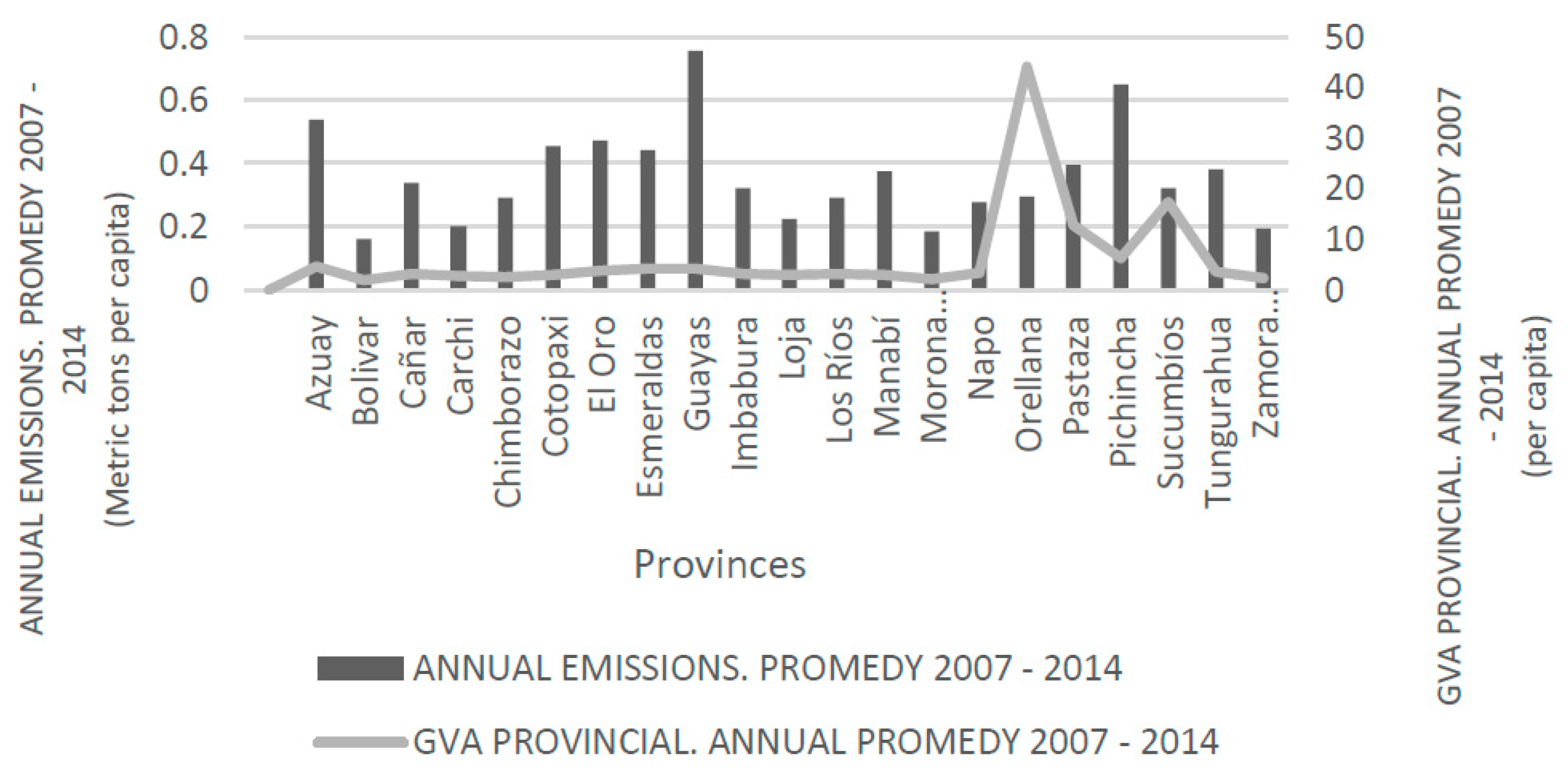
Figure 2 shows the relationship between CO2 emissions and provincial GVA averages for the 2007–2014 period. The data highlights that the electricity consumption by province is proportional to the number of inhabitants, so in 2014 the demand for energy in the most populated provinces was 7193.68 GWh in Guayas and 4015.81 GWh in Pichincha. Consequently, the level of CO2 emissions is also higher in the most populated provinces. For the same year, in Guayas, it was 0.84 tons per capita and in Pichincha it was 0.67 tons per capita, while in the oil provinces it was 0.38 tons per capita for both Orellana and Sucumbíos.
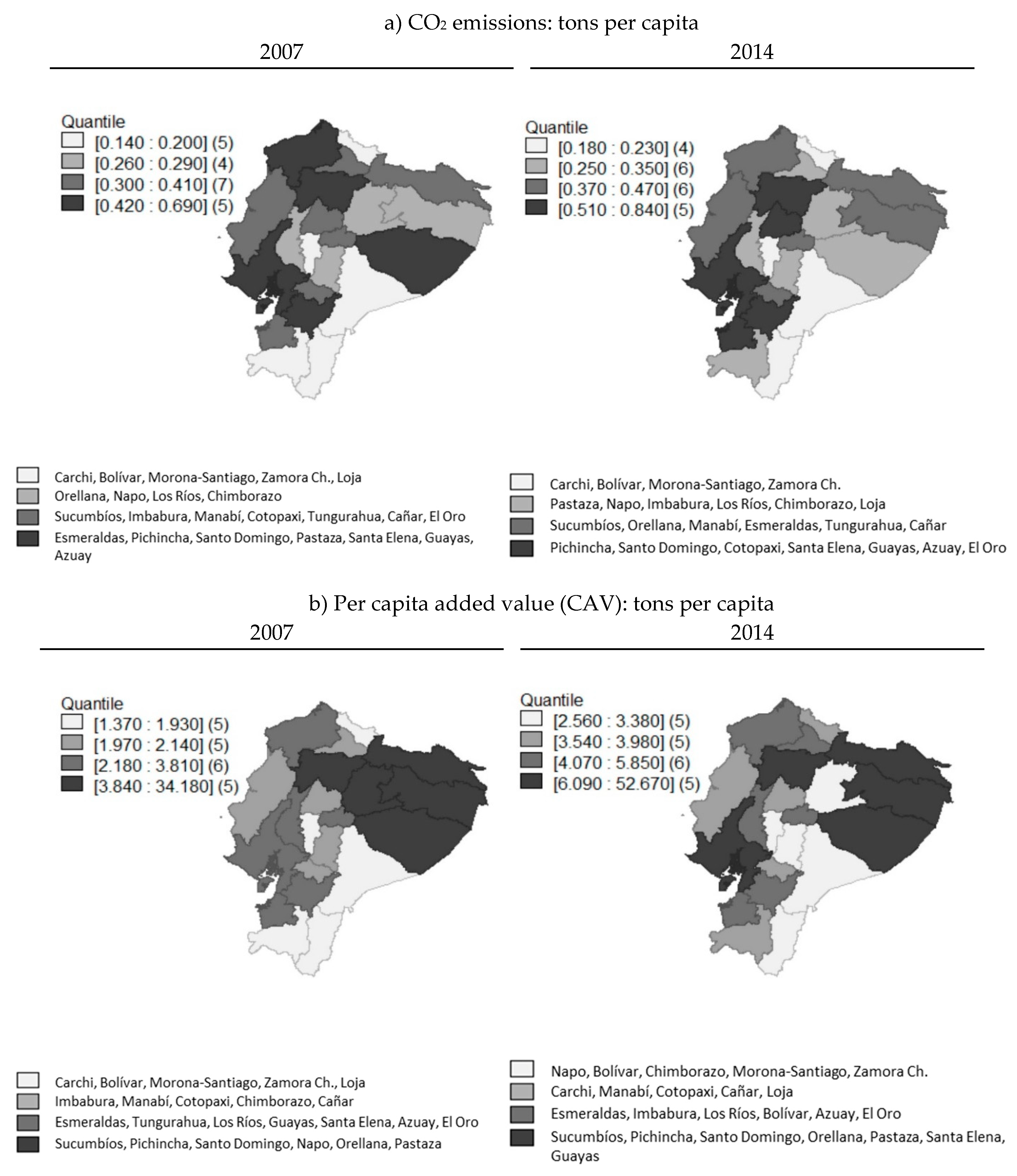
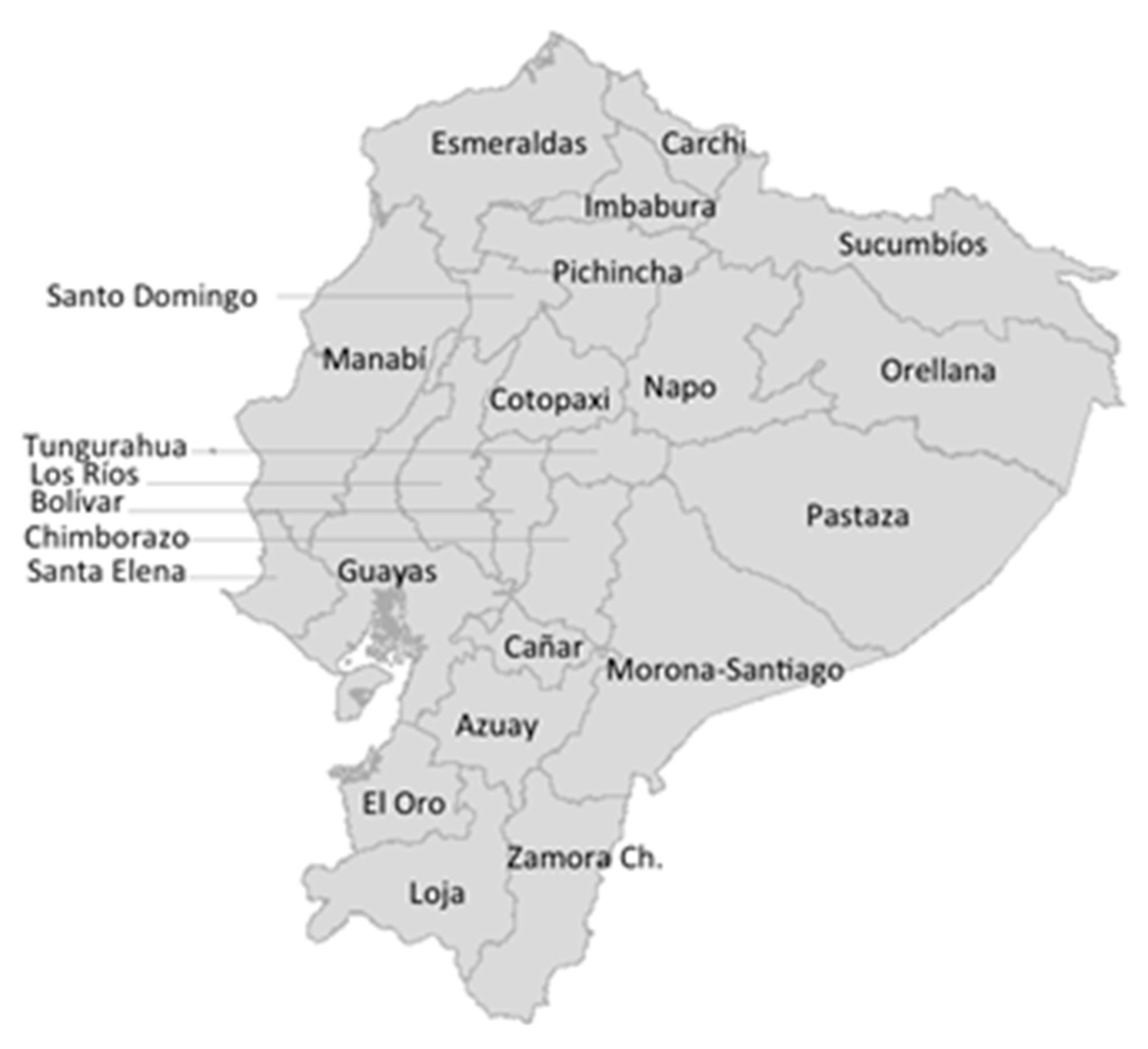
Figure 3 shows the pattern of spatial behavior of the generation of CO2 emissions and the GVA per capita in the Ecuadorian provinces. According to the data, the CO2 emissions per capita during the 2007–2014 period increased by 14%, going from 7.25 to 8.28 in those seven years. This situation resulted in the country being ranked 120 out of 185 nations arranged from the least to the most pollutant countries. At the regional level, the provinces that generated the most carbon dioxide emissions in 2007 were those with the highest concentration of industries, Guayas, Pichincha, and Azuay, together with the regions linked to oil exploitation and refining such as Pastaza and Esmeraldas. In 2014, due to the drop in international oil prices and the corresponding decrease in their related activities, these last two oil provinces decreased their CO2 emissions. As a result of the significant evolution of economic growth in the provinces of Cotopaxi and El Oro, they are among the biggest pollutants, together with Guayas, Pichincha, and Azuay (Figure 4).
Both in 2007 and in 2014, per capita production was higher in the eastern provinces where Ecuadorian crude is exploited, which shows the dependence of the Ecuadorian economy on oil. However, this apparent wealth does not correspond to reality, given that it is paradoxical that in general terms, the regions that produce the most, and where oil is exploited, are the regions where the majority of their population are lacking conditions to tackle the poverty problem. In addition, surpluses from export earnings benefited, especially since the 1970s, the two largest cities (Guayaquil and Quito), which concentrate the main economic activities of the country [55] (p.42). In 2014, the provinces with a high poverty level are the eastern provinces of Napo, Pastaza, and Morona Santiago, as well as the central province of Guaranda and Esmeraldas in the north of the Ecuadorian coast.

3. Environmental Kuznets Curve (EKC) and Carbon Kuznets Curve (CKC)

3.1. Conceptualization EKC and CKC

In those studies that address the relationship between economic growth, energy consumption, and CO2 emissions, the authors divide the specialized literature into three lines of study: “the study of the relationship GDP—energy consumption or GDP—energy–CO2 emissions, including the study of causality relationships; secondly, the study of the different aspects of the EKC hypothesis; and finally, the use of scenarios to be able to conduct forecast calculations of CO2 emissions in a forthcoming period. In many works, these lines of research overlap” [48] (p.604).
This research is part of the second line of research identified and addresses the EKC model. As already mentioned, this model emerged in the early 1990s when Grossman and Krueger [7] found empirical evidence of a non-linear relationship between economic growth and environmental degradation. These authors affirm that the inverted U-shape proposed by Kuznets [23] is also applicable to environmental studies, specifically, the relationship between the increase in per capita income and environmental degradation. Thus, the EKC (bell-shaped curve) emerges.
More broadly speaking, the EKC hypothesis explains that a country, in its early stages of development, generates the necessary losses in terms of environmental quality, which will be compensated in the future with the profits that will arise once a threshold or maximum point of per capita income is exceeded. Consequently, the continuous increase of the product will cause by itself an improvement of the environmental quality [56,57]. This means that economic growth will influence the improvement of the environment in the long term.
In this sense, EKC has strong public policy implications, since both the deterioration of the environment and the improvement of environmental quality are caused by economic growth [34]. Consequently, if environmental degradation is an inevitable process in the early stages of economic growth, the best way to achieve higher quality levels in the environment is through the acceleration of economic growth [5].
In the EKC, three effects can be identified: scale, composition, and technology [22]. The scale effect is the initial process of environmental deterioration, which occurs in the early growth stages of countries with low income levels. The composition effect involves economic growth modifying the productive structure, strengthening the services sector, which is less pollutant than the industry. Finally, the technology effect enables to establish that the most developed nations have greater capacity to invest in innovation and development of clean technologies, so, the scale effect will decrease over time. When an economy achieves the maximum level of development, composition and technology effects take place. Consequently, environmental deterioration is restored and the income continues to increase [58].
The relationship between environmental deterioration and growth established by the EKC should not be seen as a process of inevitable and automatic relationships, insofar as it should be considered that if environmental goods and services are used as consumer goods and input in the production process, it is necessary to weigh their corresponding income elasticity [59,60,61,62]. It should also be noted that the improvement of environmental quality as a need is a priority only for individuals who have met their basic needs for food, housing, and health. Thus, those people who have an adequate quality of life will give greater value to environmental goods and services, and their willingness to pay for them will be greater than the increase in their income [63].
In addition, the most developed societies have better levels of education and technical skills, which implies a higher level of demand when designing public policy and regulatory and monitoring mechanisms [64]. People living in rural sectors depend directly on natural resources and are most affected by the variation in their quantity or quality. Therefore, these people demand a better environmental quality regardless of their income level; their willingness to pay is high. However, their ability to pay depends on their income [65,66].
It should be noted that developed countries have a robust regulatory and institutional framework, so environmental regulation and the degree of trade openness tends to be stronger than in less developed countries [67,68,69]. Therefore, less developed countries are the preferred countries when it comes to locating pollution-intensive industries, which can lead to the existence of pollution havens, even if the income levels have exceeded the threshold established by the EKC [70].
This discussion has given rise to the hypothesis of the CKC, which is derived from the EKC. Its study is decisive to design public policy that enables to counteract the effects of climate change. Since climate change is a global problem [71], it is incomprehensible that only developed countries have a robust institutional framework in environmental aspects, while less developed countries are considered to be pollution havens and are more vulnerable to the effects of climate change.

3.2. Empirical Evidence

Those studies that have been conducted internationally on CKC show contradictory evidence regarding the relationship between the amount of CO2 emissions and the gross domestic product (GDP). In this sense, there are several studies, in addition to those already mentioned in the introduction of this research, which corroborated the EKC hypothesis because a non-linear inverted U-shaped relationship was found between economic growth and CO2 emissions in both the long run and short run [34,42,72,73,74,75,76,77,78,79]. Other studies only found long-term evidence and not short-term evidence [75,80]. Dinda and Coondoo [81], as well as Zilio [70], conclude that there is no long-term relationship.
The results of the research have undeniably depended on the methodology, the data used (variables to be analyzed), and the field of study (country). In this sense, Mahmudul et al. [36] (p.467), in their research, also make a relevant review on some explanations provided in the literature on the variables that affect this disparity of results.
Studies conducted in a single country and using time series found empirical evidence of the existence of the EKC hypothesis: Saboori et al. [42] (Malaysia); Esteve and Tamarit [25] (Spain); Nasir and Ur-Rehman [75] (Pakistan); He and Richard [40] (Canada); Xuemei et al. [77] (Shandong province of China); and Kanjilal and Ghosh [78] (India).
Studies conducted in a single country and using time series that did not find empirical evidence of the existence of the EKC hypothesis: Ozturk and Al-Mulali [82] (Cambodia); Al-Mulali et al. [83] (Vietnam); Akbostancı et al. [84] (Turkey); Fodha and Zaghdoud [26]; Mhenni [85] (Tunisia); Robalino-López et al. [46] (Venezuela).
Comparative studies between countries using the cross-sectional or panel data analysis that found empirical evidence of the existence of the EKC hypothesis: Narayan and Narayan [74] (43 developing countries); Apergis and Ozturk [86] (14 Asian countries); Al-Mulali et al. [87] (Latin America and the Caribbean); Bertinelli and Strobl [88].
Comparative studies between countries using the cross-sectional or panel data analysis that did not find empirical evidence of the existence of the EKC hypothesis: Jebli et al. [89] (25 OECD countries); Arouri et al. [20] (12 countries from the Middle East and North Africa); Musolesi et al. [32] (106 developed and developing countries); Jaunky [90] (36 high income countries).
Studies carried out in comparative studies between countries using cross-sectional or panel data analysis whose results indicate different causality relationships for the different countries: Coondoo and Dinda [91] and Mahmudul et al. [36].
Few studies have been conducted for Ecuador, so Robalino-López et al. [46] use cointegration techniques to evaluate the existence of the EKC hypothesis in the medium term using Jaunky´s specification. Although their results do not show compliance with the EKC, they do show evidence that Ecuador could be on track to achieve environmental stability in the near future, if economic growth is combined with an increase in the use of renewable energies, an improvement of productivity, sectoral structure and the use of a more efficient fossil fuel technology.
White Zambrano-Monserrate et al. [49] apply cointegration tests, stability tests, and causality of Granger, which allows them to confirm the presence of the EKC in the long term, but not in the short term. This would show that Ecuador is still in the ascending part of the curve. In addition, Almeida [47] concludes that for the 1970–2010 period, per capita income generated positive and negative effects on the amount of CO2 emissions and verifies the existence of EKC through econometric modelling.

4. Methodology

4.1. Study Variables

In the regression model to be estimated, emissions of carbon dioxide (CO2) per capita, measured in tons per person, will be considered as a variable dependent on environmental deterioration. It is necessary to mention that in Ecuador there is no provincial information related to CO2 emissions during the study period, therefore, energy consumption and the CO2 emission factor are used as a proxy variable. Table 1 shows the data used and the corresponding information sources. While the provincial production will be the main independent variable, for the present case the provincial GVA is used per as a proxy variable of production in the provinces, the series have been taken from the provincial accounts of the Central Bank of Ecuador for the 2000–2014 period [53].
The model is complemented with control variables such as the number of vehicles, schooling, and the GINI coefficient [22,31]. In the Equation estimation (4)—see methodology—the following control variables will be used:
  • The number of vehicles per capita (VEHICLESPC). The series for the 2007–2014 period was obtained from transportation statistics at provincial level of the National Institute of Statistics and Census [92].
  • The poverty index by income (PO). It is provided by the survey of employment, unemployment, and underemployment that the National Institute of Statistics and Census (INEC) performs annually [52,93,94].
  • Years of schooling by province (SCH). They are obtained from the System of Social Indicators of Ecuador [95].
  • The provincial Gini coefficient (GINI). It was calculated based on the national employment and unemployment surveys (ENEMDU) surveys [52,93,94].
The aim of these control variables is to observe the effects that poverty and inequality could have on the generation of pollutant emissions, in addition to including the educational level to confirm the premise that societies with a higher educational level tend to take more care of the environment.
In this study, the variables of 21 of the 24 Ecuadorian Provinces are taken into account. Galápagos was not considered because it is an insular region outside the continent, which does not allow for involving it in the spatial methods (neighborhood effect and contiguity) used in this study, as Quintana et al. [96] points out. However, in the data of the provinces of Santo Domingo and Santa Elena, Pichincha, and Guayas were incorporated, respectively, since they are of recent creation (year 2009, before this year they were administratively part of Pichincha and Guayas), so it is not possible to have provincial accounts for previous years.

4.2. Empirical Analysis Model for CKC Estimation

In the empirical analyses on the existence of CKC, different econometric methodologies were used, in which the most common specification was to consider some type of pollutant emission (Cont) as the dependent variable and to relate it to production (Prod), the square of the production (Prod2), and a random perturbation term (u) in a regression model, as described in Equation (1):
C o n t t = β 1 + β 2 P r o d t + β 3 P r o d 2 t + u t
where t is the time and β 1 , β 2 and β 3 are the unknown parameters of the model.
In panel models, the specification changes slightly by including cross-sectional observations indexed with the letter i in each period of time and adding a term of unobservable fixed effects μ i [97,98]:
C o n t i t = μ i + β 1 + β 2 P r o d i t + β 3 P r o d 2 i t + u i t
The relationship between pollutant emissions and production is conditioned to the effect that other variables (X) could have on pollution, the inclusion of these variables is shown in Equation (3).
C o n t i t = μ i + β 1 + β 2 P r o d i t + β 3 P r o d 2 i t + i = 1 p γ i X i + u i t
The specification of Equation (1) has been used in time series models, whereas (2) and (3) have been used when different countries or regions are included, so this last specification is taken up again and the following model is proposed:
C 02 i t = μ i + β 1 + β 2 G V A P C i t + β 3 G V A P C 2 i t + γ 1 V E H I C L E S P C i t + γ 2 P P I i t + γ 3 S C H i t + γ 4 G I N I i t + u i t
where: CO2 = Carbon dioxide emissions per capita; GVAPC = gross value added per capita; GVAPC2 = gross value added per capita squared; VEHICLESPC = number of vehicles per capita; PPI = provincial poverty index; SCH = years of schooling by province; GINI = provincial GINI coefficient; i = 1,2, …,21; and t = 2007, 2008, …, 2014, i.e., the information used in this work corresponds to observations for the 2007–2014 period, considering a set of 21 provinces of Ecuador.
Due to the fact that the analysis is carried out considering geographic units, i.e., Ecuadorian provinces, Equation (4) could have a specification error by not taking into account the possible existence of spatial dependence of the variables, as it has been widely argued in the literature on spatial econometrics [99,100,101,102].
In order to avoid the possible existence of a specification error, model (4) was also estimated as a spatial panel, as shown in Equation (5):
C 02 i t = μ i + β 1 + β 2 G V A P C i t + β 3 G V A P C 2 i t + γ 1 V E H I C L E S P C i t + γ 2 P P I i t + γ 3 S C H i t + γ 4 G I N I i t + ρ W C 02 i t + θ 1 W G V A P C i t + θ 2 W G V A P C 2 i t + θ 3 W V E H I C L E S P C i t + θ 4 W P P I i t + θ 5 W S C H i t + θ 6 W G I N I i t + u i t u i t = λ W u i t + ε i t
where W is a spatial weight matrix, ρ is the coefficient of autoregressive spatial lag, θ i are the parameters of the spatial lags of the explanatory variables of the model, λ is the spatial lag coefficient of the errors, and ε i t is a random disturbance term. The specification of Equation (5) follows the methodology of spatial panel models proposed by Anselin [100], which goes from the particular to the general, taking the classical panel model (Table 2) as a starting point. Subsequently, the model coefficients are tested in order to incorporate spatial effects until reaching the more general model as a starting point, which Elhorst [103] denominates the general nested space model (MEGA).
Under a methodology from the particular to the general and from a hypothesis testing process, it is possible to give rise to a wide variety of spatial models whose characteristics can be consulted in Elhorst [103] and the different variants estimated in this document were the following:
Spatial auto regression (SAR) model:
C 02 i t = μ i + β 1 + β 2 G V A P C i t + β 3 G V A P C 2 i t + γ 1 V E H I C L E S P C i t + γ 2 P P I i t + γ 3 S C H i t + γ 4 G I N I i t + ρ W C 02 i t + u i t u i t = ε i t
Spatial simultaneous autoregressive SAC model:
C 02 i t = μ i + β 1 + β 2 G V A P C i t + β 3 G V A P C 2 i t + γ 1 V E H I C L E S P C i t + γ 2 P P I i t + γ 3 S C H i t + γ 4 G I N I i t + ρ W C 02 i t + u i t u i t = λ W u i t + ε i t
Structural equation modeling (SEM):
C 02 i t = μ i + β 1 + β 2 G A V P C i t + β 3 G A V P C 2 i t + γ 1 V E H I C L E S P C i t + γ 2 P P I i t + γ 3 S C H i t + γ 4 G I N I i t + u i t u i t = λ W u i t + ε i t
Generalized spatial panel random effects (GSPRE) model:
C 02 i t = μ i + β 1 + β 2 G V A P C i t + β 3 G V A P C 2 i t + γ 1 V E H I C L E S P C i t + γ 2 P P I i t + γ 3 S C H i t + γ 4 G I N I i t + u i t u i t = λ W u i t + ε i t μ i = ϕ μ i + α i

5. Results and Interpretation of the CKC Models

The results of the estimation of Equation (4) are shown in Table 2. With the exception of poverty and the Gini index, all the other variables are statistically significant. The signs of the variables are adequate and correspond to what is stated by the theory: when the number of vehicles per capita increases (VEHICLESPC), emissions increase, as schooling increases, pollution decreases (SCH), and the EKC is fulfilled since income (GVAPC) is statistically significant and positive, while its square (GVAPC2) is negative and significant. The results are consistent both with the fixed and random effects model, and the values obtained for the coefficients of both models are very similar.
Spatial dependence tests were performed on the variables by using the Moran Index, which is expressed as follows:
I = R i j w i j i j w i j ( x i x ¯ ) ( x j x ¯ ) i ( x i x ¯ ) 2
where x i is the study variable in region i, x ¯ is its sample mean, w i j are the weights of the W matrix, and R is the sample size (number of provinces).
A significant positive (negative) value of the Moran index will lead to the rejection of the null hypothesis of non-spatial dependence and the acceptance of positive (negative) spatial dependence.
Figure 5 shows the overall and local results of the Moran index for CO2 emissions in Ecuadorian provinces. The results show that this index is significant for CO2 emissions and that it tends to become positive over time.
As spatial dependence was significant, estimates of the different models formulated in Equations (5)–(9) were performed. The results obtained are shown in Table 3.
Following the methodology of the general to the particular in the last two columns of Table 3, the results for Equation (5) are shown, both for the spatial panel model of fixed effects and of random effects. The results of both models are highly satisfactory, in both cases the spatial effects are significant, and the results are similar.
The spatial lag on CO2 emissions is significant and shows that there are spatial spillover effects, which means that when CO2 emissions increase in one of the provinces, this positively affects the emissions of its neighbors. It is relevant that spatially lagged explanatory variables are significant for the value added per capita, its square and for the vehicle fleet per person. In particular, the spatial lag effects on vehicles are negative, which means that when the vehicle fleet increases in one of the provinces, the emissions from the neighboring provinces are reduced. In addition, when the value added per person increases in the neighboring provinces, emissions in a specific province are reduced. The same as in the case of the model without spatial effects of Table 2, the results confirm compliance with the CKC.
In the rest of the models, the results are also very consistent to establish compliance with the CKC. However, they have a specification error problem, as they omit a set of relevant variables, which in this case are spatially lagged explanatory variables that are significant in the species distribution modelling (SDM models). For this reason and considering that in the face of a specification error problem, the coefficients of the model are not consistent, the decision was to select SDM models as the most appropriate representation of the process that explains the generation of pollutant emissions in the Ecuadorian provinces.
In order to evaluate the spatial dynamics in CO2 generation, the results for the spatial impact multipliers are shown in Table 4. It is important to consider that these multipliers are obtained from the following transformation in the SDM spatial model [102]:
( I n ρ W ) y = X β + W X θ + ι n + u y = r = 1 k S r ( W ) x r + V ( W ) ι n μ + V ( W ) u S r ( W ) = V ( W ) ( I n β r + W θ r ) V ( W ) = ( I n ρ W ) 1 = I n + ρ W + ρ 2 W 2 + ρ 3 W 3 +
where S r ( W ) is the matrix of total spatial impacts and V ( W ) shows the expansion of spatial impacts for first order and higher order neighborhoods.
Equation (11) shows that region i will impact region j and then j will impact region i, resulting in a sequence of impacts. In the case of Equation (5), this implies that the variations in CO2 emissions in a region depend on the emissions in the neighboring regions (Wy) and the other variables (vehicles, education, etc.) in the neighboring regions (WX).
Table 4 shows the results of the spatial impact multipliers, in which it is highlighted that the direct and indirect effects are of opposite signs, which generates a compensation of impacts. This means that neighborhood effects tend to compensate for changes in the generation of pollutant emissions. For example, when production in a region increases, causing greater pollution, in the neighboring regions the effect is compensated by generating less pollution, which results in a net effect that is compensated. The other relevant characteristic is that the main variable that affects the dispersion effects of pollution by provinces is the number of vehicles and it is the only variable whose direct and indirect effects are not compensated, giving rise to a positive and significant net effect on the CO2 emission.

6. Conclusions

This document aims to fill the gap that exists in the literature regarding CO2 emissions, as a consequence of electricity consumption in the provinces of Ecuador. The results of this work constitute an important contribution for the design of public policies related to energy efficiency and reduction of environmental pollution. In addition, it contributes to the literature on EKC with a novel study at the regional level. Among the limitations of the study, note that given the difficulty to obtain total data on CO2 emissions at provincial level of the industrial and agricultural sectors, only electricity consumption data were used.
The empirical evidence presented in this investigation reveals that for the 21 provinces of Ecuador, during the 2007–2014 period, by means of a panel data model, EKC, in an inverted U-shape is fulfilled since income is statistically significant and positive, while its square is negative and significant.
The EKC hypothesis, as already mentioned, explores the relationship between economic growth and environmental deterioration. Therefore, in the short-term, economic growth causes an environmental deterioration and in the long-term, this growth leads to an improvement of the environment, as well as a reduction of its deterioration. In the long-term, production processes use more efficient technologies that involve the conservation of natural resources.
The same results are obtained and show a high consistency when different specifications of spatial panel econometric models are made. In all cases, increases in per capita production lead to an increase in pollutant emissions. However, in the long term, growth has led to a process of reducing emissions, which can be seen in the negative sign of the square of the production variable. This means that the Ecuadorian provinces have exceeded the critical threshold of income in terms of pollutant emissions.
In this investigation, it is observed that when the number of cars per capita increases, emissions increase, as schooling rises, pollution decreases. Although the results do not show a constant deterioration in environmental quality due to the growth of the economy, there is evidence that the evolution of urban and city life, reflected in the increase in the per capita vehicle fleet, becomes a significant factor of the environmental deterioration of Ecuadorian provinces. The estimates of the spatial models indicate that vehicles are a significant factor in CO2 emissions and their total impact also has a neighborhood effect among the different provinces of the country. On the other hand, higher levels of education tend to reduce CO2 emissions, which confirms the idea that a more educated population is more aware of the problem and contributes to polluting less. Finally, space spill effects were observed, so as CO2 emissions rise in a province, it affects positively to the emissions of its neighbors.
Based on the results obtained, it is possible to state that public policies can play an active role in the environmental improvement of the country if they focus on finding alternative means of transport to cars and are more concerned with increasing the educational level of the population. This is consistent with what Robalino-López [48] proposed, who emphasizes the need to implement policies that allow for the diversification of energy sources and increase energy efficiency in productive sectors to achieve more sustainable development.

Author Contributions

All authors contributed equally to this work. All authors wrote, reviewed and commented on the manuscript. All authors have read and agreed to the published version of the manuscript.

Funding

This research received no external funding.

Conflicts of Interest

The authors declare no conflict of interest.

References

  1. European Commission. Available online: https://ec.europa.eu/clima/change/causes_en (accessed on 2 January 2019).
  2. Intergovernmental Panel on Climate Change. Climate Change 2007: Summary Report. Intergovernmental Group of Experts on Climate Change 2007. Available online: https://www.ipcc.ch/pdf/assessment-report/ar4/syr/ar4_syr_sp.pdf (accessed on 2 January 2019).
  3. International Energy Agency. CO2 Emissions from Fuel Combustion Highlights 2011. Available online: http://www.iea.org/media/statistics/co2highlights.pd (accessed on 2 January 2019).
  4. Ministry of Environment. Inventory of Greenhouse Gases. Homepage 2015. Available online: http://www.ambiente.gob.ec/ (accessed on 17 January 2019).
  5. Beckerman, W. Economic growth and the environment: Whose growth? Whose environment? World Dev. 1992, 20, 481–496. [Google Scholar] [CrossRef]
  6. Panayotou, T. Empirical Tests and Policy Analysis of Environmental Degradation at Different Stages of Economic Development; Working Paper WP238 Technology and Employment Programme; International Labor Office: Geneva, Switzerland, 1993. [Google Scholar]
  7. Grossman, G.M.; Krueger, A.B. Environment Impacts of a North American Free Trade Agreement. In The Mexican-US Free Trade Agreement; Garber, P.M., Ed.; MIT Press: Cambridge, MA, USA, 1993. [Google Scholar]
  8. Arrow, K.; Bolin, B.; Costanza, R.; Dasgupta, P.; Folke, C.; Helling, C.S.; Jansson, B.O.; Levin, S.; Mailer, K.G.; Perrings, C.; et al. Economic growth, carrying capacity, and the environment. Science 1995, 268, 520–521. [Google Scholar] [CrossRef] [PubMed]
  9. Stern, D.I.; Cleveland, C.J. Energy and Economic Growth; Rensselaer Polytechnic Institute, Rensselaer Working Papers in Economics No.0410; Rensselaer Polytechnic Institute: Troy, NY, USA, 2004. [Google Scholar]
  10. Weber, C.L.; Peters, G.P.; Guan, D.; Hubacek, K. The contribution of Chinese exports to climate change. Energy Policy 2008, 36, 3572–3577. [Google Scholar] [CrossRef] [Green Version]
  11. Dean, J.M.; Signoret, J.; Feinberg, R.; Ludema, R.D.; Ferrantino, M.J. Estimating the Price Effects of Non-Tariff Barriers. J. Econ. Anal. Policy 2009, 9, 1–41. [Google Scholar] [CrossRef]
  12. Payne, J.E. Survey of the international evidence on the causal relationship between energy consumption and growth. J. Econ. Stud. 2010, 37, 53–95. [Google Scholar] [CrossRef]
  13. Jordan, B.R. The Environmental Kuznets Curve: Preliminary Meta-Analysis of Published Studies, 1995–2010; Georgia Tech School of Public Policy Workshop on Original Policy Research (WOPR); Georgia Tech School of Public Policy: Atlanta, GA, USA, 2010. [Google Scholar]
  14. Kim, J.; Li, S.; Kim, K.R.; Stohl, A.; Mühle, J.; Kim, S.K.; Salameh, P.K. Regional atmospheric emissions determined from measurements at Jeju Island, Korea: Halogenated compounds from China. Geophys. Res. Lett. 2010, 37, 1–5. [Google Scholar] [CrossRef] [Green Version]
  15. Menyah, K.; Wolde-Rufael, Y. CO2 emissions, nuclear energy, renewable energy and economic growth in the US. Energy Policy 2010, 38, 2911–2915. [Google Scholar] [CrossRef]
  16. Yunfeng, Y.; Laike, Y. China’s foreign trade and climate change: A case study of CO2 emissions. Energy Policy 2010, 38, 350–356. [Google Scholar] [CrossRef]
  17. Hang, G.; Jiang, Y.-S. The relationship between CO2 emissions, economic scale, technology, income and population in China. Procedia Environ. Sci. 2011, 11, 1183–1188. [Google Scholar] [CrossRef] [Green Version]
  18. Pao, H.T.; Tsai, C.M. Multivariate Granger causality between CO2 emissions, energy consumption, FDI (foreign direct investment) and GDP (gross domestic product): Evidence from a panel of BRIC (Brazil, Russian Federation, India, and China) countries. Energy 2011, 36, 685–693. [Google Scholar] [CrossRef]
  19. Alam, M.J.; Begum, I.A.; Buysse, J.; Van Huylenbroeck, G. Energy consumption, carbon emissions and economic growth nexus in Bangladesh: Cointegration and dynamic causality analysis. Energy Policy 2012, 45, 217–225. [Google Scholar] [CrossRef]
  20. Arouri, M.E.H.; Youssef, A.B.; M’henni, H.; Rault, C. Energy consumption, economic growth and CO2 emissions in Middle East and North African countries. Energy Policy 2012, 45, 342–349. [Google Scholar] [CrossRef] [Green Version]
  21. Saboori, B.; Sapri, M.; Bin Baba, M. Economic growth, energy consumption and CO2 emissions in OECD (Organization for Economic Co-operation and Development)’s transport sector: A fully modified bi-directional relationship approach. Energy 2014, 66, 150–161. [Google Scholar] [CrossRef]
  22. Grossman, G.M.; Krueger, A.B. Environmental Impacts of a North American Free Trade Agreement; Papers 158; Woodrow Wilson School-Public and International Affairs: Princeton, NJ, USA, 1991. [Google Scholar]
  23. Kuznets, S. Economic growth and income inequality. Am. Econ. Rev. 1955, 45, 1–28. [Google Scholar]
  24. Wagner, M. The carbon Kuznets curve: A cloudy picture emitted by bad econometrics? Resour. Energy Econ. 2008, 30, 388–408. [Google Scholar] [CrossRef] [Green Version]
  25. Esteve, V.; Tamarit, C. Is there an environmental Kuznets curve for Spain? Fresh evidence from old data. Econ. Model. 2012, 29, 2696–2703. [Google Scholar] [CrossRef]
  26. Fodha, M.; Zaghdoud, O. Economic growth and pollutant emissions in Tunisia: An empirical analysis of the environmental Kuznets curve. Energy Policy 2010, 38, 1150–1156. [Google Scholar] [CrossRef]
  27. Holtz-Eakin, D.; Selden, T.M. Stoking the fires? CO2 emissions and economic growth. J. Public Econ. 1995, 57, 85–101. [Google Scholar] [CrossRef] [Green Version]
  28. Lantz, V.; Feng, Q. Assessing income, population, and technology impacts on CO2 emissions in Canada: where’s the EKC? Ecol. Econ. 2006, 57, 229–238. [Google Scholar] [CrossRef]
  29. Omri, A. CO2 emissions, energy consumption and economic growth nexus in MENA countries: Evidence from simultaneous equations models. Energy Econ. 2013, 40, 657–664. [Google Scholar] [CrossRef] [Green Version]
  30. Grossman, G.M.; Krueger, A.B. Economic growth and the environment. Q. J. Econ. 1995, 110, 353–377. [Google Scholar] [CrossRef] [Green Version]
  31. Poudel, B.; Paudel, K.; Bhattarai, K. Searching for an Environmental Kuznets Curve in Carbon Dioxide Pollutant in Latin American Countries. J. Agric. Appl. Econ. 2009, 41, 3–27. [Google Scholar] [CrossRef] [Green Version]
  32. Musolesi, A.; Mazzanti, M.; Zoboli, R. A panel data heterogeneous Bayesian estimation of environmental Kuznets curves for CO2 emissions. Appl. Econ. 2010, 42, 2275–2287. [Google Scholar] [CrossRef] [Green Version]
  33. De Bruyn, S.M.; van den Bergh, J.C.; Opschoor, J.B. Economic growth and emissions: Reconsidering the empirical basis of environmental Kuznets curves. Ecol. Econ. 1998, 25, 161–175. [Google Scholar] [CrossRef]
  34. Galeotti, M.; Lanza, A.; Pauli, F. Reassessing the Environmental Kuznets Curve for CO2: A robustness exercise. Ecol. Econ. 2006, 57, 431–455. [Google Scholar] [CrossRef]
  35. Begum, R.A.; Sohag, K.; Abdullah, S.M.S.; Jaafar, M. CO2 emissions, energy consumption, economic and population growth in Malaysia. Renew. Sustain. Energy Rev. 2015, 41, 594–601. [Google Scholar] [CrossRef]
  36. Mahmudul, H.M.; Hagos, F.Y.; Mamat, R.; Abdullah, A.A.; Awad, O.I. Experimental investigation of the impact of using alcohol-biodiesel-diesel blending fuel on combustion of single cylinder CI engine. In IOP Conference Series: Materials Science and Engineering; IOP Publishing: Bristol, UK, 2016; p. 012038. [Google Scholar]
  37. Selden, T.M.; Song, D. Environmental quality and development: Is there a Kuznets curve for air pollution emissions? J. Environ. Econ. Manag. 1994, 27, 147–162. [Google Scholar] [CrossRef]
  38. Ekins, P. The Kuznets curve for the environment and economic growth: Examining the evidence. Environ. Plan. 1997, 29, 805–830. [Google Scholar] [CrossRef] [Green Version]
  39. Iglesias-Rodríguez, M.D.; Halloran, P.R.; Rickaby, R.E.M.; Hall, I.R.; Colmenero-Hidalgo, E.; Gittins, J.R.; Green, D.R.H.; Tyrell, T.; Gibbs, S.J.; von Dassow, P.; et al. Phytoplankton calcification in a high-CO2 world. Science 2008, 320, 336–340. [Google Scholar] [CrossRef] [Green Version]
  40. He, J.; Richard, P. Environmental Kuznets curve for CO2 in Canada. Ecol. Econ. 2010, 69, 1083–1093. [Google Scholar] [CrossRef] [Green Version]
  41. Pao, H.T.; Tsai, C.M. CO2 emissions, energy consumption and economic growth in BRIC countries. Energy Policy 2010, 38, 7850–7860. [Google Scholar] [CrossRef]
  42. Saboori, B.; Sulaiman, J.; Mohd, S. Economic growth and CO2 emissions in Malaysia: A cointegration analysis of the environmental Kuznets curve. Energy Policy 2012, 51, 184–191. [Google Scholar] [CrossRef]
  43. World Bank. World Development Indicators: Ecuador; World Bank Group: Washington, DC, USA, 2017; Available online: https://datos.bancomundial.org/pais/ecuador (accessed on 14 January 2019).
  44. Roca, J.; Padilla, E.; Farré, M.; Galletto, V. Economic growth and atmospheric pollution in Spain: Discussion the environmental Kuznets hypothesis. Ecol. Econ. 2001, 39, 85–99. [Google Scholar] [CrossRef] [Green Version]
  45. Mills, J.H.; Waite, T.A. Economic prosperity, biodiversity conservation, and the environmental Kuznets curve. Ecol. Econ. 2009, 68, 2087–2095. [Google Scholar] [CrossRef]
  46. Robalino-López, A.; García-Ramos, J.; Golpe, A.; Mena-Nieto, A. System dynamics modelling and the environmental Kuznets curve in Ecuador (1980–2025). Energy Policy 2014, 67, 923–931. [Google Scholar] [CrossRef] [Green Version]
  47. Almeida, D. Crecimiento Económico y Medio Ambiente: La Curva Ambiental de Kuznets para el Ecuador en el Periodo 1970–2010 (tesis de grado); Pontificia Universidad Católica del Ecuador: Quito, Ecuador, 2013. [Google Scholar]
  48. Robalino-López, A.; Mena-Nieto, A.; García-Ramos, J.; Golpe-Moya, A. Studying the relationship between economic growth, CO2 emissions, and the environmental Kuznets curve in Venezuela (1980–2025). Renew. Sustain. Energy Rev. 2015, 41, 602–614. [Google Scholar] [CrossRef] [Green Version]
  49. Zambrano-Monserrate, M.; García–Albán, F.; Henk-Vera, K. Bounds testing approach to analyze the existence of an environmental Kuznets curve in Ecuador. Int. J. Energy Econ. Policy 2016, 6, 159–166. [Google Scholar]
  50. Correa-Quezada, R.; Ochoa, F.; Quinche, P. Creatividad y clase creativa en Ecuador. In La economía de las actividades creativas: Una perspectiva desde España y México; Copublication CRIM-UNAM-Universidad Alcalá: Madrid, Spain, 2017; pp. 435–490. [Google Scholar]
  51. Villacís, B.; Carrillo, D. País atrevido: La Nueva Cara Sociodemográfica del Ecuador. Instituto Nacional de Estadística y Censos (INEC). Edición Especial Revista Analitika. Quito–Ecuador. 2012. Available online: http://www.ecuadorencifras.gob.ec/wp-content/descargas/Libros/Economia/Nuevacarademograficadeecuador.pdf (accessed on 14 January 2019).
  52. INEC. Population and Demography. National Institute of Statistics and Census. 2014. Available online: http://www.ecuadorencifras.gob.ec/directorio-de-empresas-2014/ (accessed on 2 January 2019).
  53. Central Bank of Ecuador. Regional National Accounts 2007–2014; BCE: Quito, Ecuador, 2018; Available online: https://www.bce.fin.ec/index.php/component/k2/item/293-cuentas-provinciales/ (accessed on 22 January 2019).
  54. ARCONEL-MEER. Agency for Regulation and Control of Electricity Annual and Multiannual Statistics of the Ecuadorian Electric Sector. Republic of Ecuador. 2015. Available online: https://www.regulacionelectrica.gob.ec/boletines-estadisticos/ (accessed on 22 January 2019).
  55. Correa-Quezada, R.; Bonilla, J. Modelos de desarrollo en Ecuador: Una revisión desde la Colonia a la Actualidad. In Realidad Nacional. Coordinadores Ronny Correa-Quezada y Tangya Tandazo-Arias; Universidad Técnica Particular de Loja. Ediloja Cia. Ltda: Loja, Ecuador, 2018; pp. 15–56. [Google Scholar]
  56. Stern, D.I.; Common, M.S. Is there an environmental Kuznets curve for sulphur? J. Environ. Econ. Manag. 2001, 41, 162–178. [Google Scholar] [CrossRef] [Green Version]
  57. Catalán, H. Curva ambiental de Kuznets: Implicaciones para un crecimiento sustentable. Economía Informa 2014, 389, 19–37. [Google Scholar] [CrossRef] [Green Version]
  58. Rothman, D.S. Environmental Kuznets curves: Real progress or passing the buck? A case for consumption-based approaches. Ecol. Econ. 1998, 25, 177–194. [Google Scholar] [CrossRef]
  59. Tilton, J.E. World Metal Demand: Trends and Prospects; Resources for the Future: Washington, DC, USA, 1990. [Google Scholar]
  60. Goldemberg, J. Energy, technology, development. Ambio 1992, 21, 14–17. [Google Scholar]
  61. Shafik, N.; Bandyopadhyay, S. Economic Growth and Environmental Quality: Time Series and Cross-Country Evidence; World Bank Publications: Herndon, VA, USA, 1992. [Google Scholar]
  62. Bruyn de, S.M. Explaining the environmental Kuznets curve: Structural change and international agreements in reducing sulphur emissions. Env. Dev. Econ. 1997, 2, 485–503. [Google Scholar] [CrossRef] [Green Version]
  63. Roca, J. Do individual preferences explain Environmental Kuznets Curve? Ecol. Econ. 2003, 45, 3–10. [Google Scholar] [CrossRef]
  64. Dasgupta, S.; Laplante, B.; Wang, H.; Wheeler, D. Confronting the Environmental Kuznets Curve. J. Econ. Perspect. 2002, 16, 147–168. [Google Scholar] [CrossRef] [Green Version]
  65. Ekins, P. Economic Growth and Environmental Sustainability: The Prospects for Green Growth; Rowtledge, Taylor and Francis Group: London, UK, 2000. [Google Scholar]
  66. Zilio, M. Curva de Kuznets ambiental: La validez de sus fundamentos en países en desarrollo. Cuadernos Economía 2012, 35, 43–54. [Google Scholar] [CrossRef]
  67. Panayotou, T. Demystifying the environmental Kuznets curve: Turning a black box into a policy tool. Environ. Dev. Econ. 1997, 2, 465–484. [Google Scholar] [CrossRef] [Green Version]
  68. Cole, M.A. Trade, the pollution haven hypothesis and environmental kuznets curve: Examining the linkages. Ecol. Econ. 2004, 48, 71–81. [Google Scholar] [CrossRef]
  69. Kearsley, A.; Riddel, M. A further inquiry into the Pollution Haven Hypothesis and the Environmental Kuznets Curve. Ecol. Econ. 2010, 69, 905–919. [Google Scholar] [CrossRef]
  70. Zilio, M. La Curva de Kuznets Ambiental: Evidencia para América Latina y el Caribe (Tesis doctoral); Universidad Nacional del Sur: Bahía Blanca, Buenos Aires, Argentina, 2011. [Google Scholar]
  71. Schelling, T.C. Some economics of global warming. Am. Econ. Rev. 1992, 82, 1–14. [Google Scholar]
  72. Martínez-Zarzoso, I.; Bengochea, A. Testing for an Environmental Kuznets Curve in Latin-American Countries. Análisis Económico 2003, 18, 3–26. [Google Scholar]
  73. Nam Kwon, M.; Roldán, A.; Quintana, L. Crecimiento económico y la contaminación medioambiental en las ciudades mexicanas. J. Iber. Latin Am. Res. 2016, 22, 31–44. [Google Scholar]
  74. Narayan, P.K.; Narayan, S. Carbon dioxide emissions and economic growth: Panel data evidence from developing countries. Energy Policy 2010, 38, 661–666. [Google Scholar] [CrossRef]
  75. Nasir, M.; Ur-Rehman, F. Environmental Kuznets Curve for carbon emissions in Pakistan: An empirical investigation. Energy Policy 2011, 39, 1857–1864. [Google Scholar] [CrossRef]
  76. Esteve, V.; Tamarit, C. Threshold cointegration and nonlinear adjustment between CO2 and income: The environmental Kuznets curve in Spain, 1857–2007. Energy Econ. 2012, 341, 2148–2156. [Google Scholar] [CrossRef]
  77. Xuemei, H.; Mingliang, Z.; Su, L. Research on the relationship of economic growth and environmental pollution in Shandong province based on environmental Kuznets curve. Energy Procedia 2011, 5, 508–512. [Google Scholar] [CrossRef] [Green Version]
  78. Kanjilal, K.; Ghosh, S. Environmental Kuznet’s curve for India: Evidence from tests for cointegration with unknown structuralbreaks. Energy Policy 2013, 56, 509–515. [Google Scholar] [CrossRef]
  79. Sephton, P.; Mann, J. Further evidence of an environmental Kuznets curve in Spain. Energy Econ. 2013, 36, 177–181. [Google Scholar] [CrossRef]
  80. Shahbaz, M.; Lean, H.H.; Shabbir, M.S. Environmental Kuznets curve hypothesis in Pakistan: Cointegration and Granger causality. Renew. Sustain. Energy Rev. 2012, 16, 2947–2953. [Google Scholar] [CrossRef] [Green Version]
  81. Dinda, S.; Coondoo, D. Income and emission: A panel data-based cointegration analysis. Ecol. Econ. 2006, 57, 167–181. [Google Scholar] [CrossRef] [Green Version]
  82. Ozturk, I.; Al-Mulali, U. Investigating the validity of the environmental Kuznets curve hypothesis in Cambodia. Ecol. Indic. 2015, 57, 324–330. [Google Scholar] [CrossRef]
  83. Al-Mulali, U.; Saboori, B.; Ozturk, I. Investigating the environmental Kuznets curve hypothesis in Vietnam. Energy Policy 2015, 76, 123–131. [Google Scholar] [CrossRef]
  84. Akbostancı, E.; Türüt-Aşık, S.; Tunç, G. The relationship between income and environment in Turkey: Is there an environmental Kuznets curve? Energy Policy 2009, 37, 861–867. [Google Scholar] [CrossRef]
  85. Mhenni, H. Economic development, adjustment and environmental quality: The case of Tunisia for a contingent valuation study. Mediterr. J. Econ. Agric. Environ. 2005, 4, 36–42. [Google Scholar]
  86. Apergis, N.; Ozturk, I. Testing environmental Kuznets curve hypothesis in Asian countries. Ecol. Indic. 2015, 52, 16–22. [Google Scholar] [CrossRef]
  87. Al-Mulali, U.; Tang, C.; Ozturk, I. Estimating the environment Kuznets curve hypothesis: Evidence from Latin America and the Caribbean countries. Renew. Sustain. Energy Rev. 2015, 50, 918–924. [Google Scholar] [CrossRef]
  88. Bertinelli, L.; Strobl, E. The Environmental Kuznets Curve Semi-parametrically Revisited. Econ. Lett. 2005, 88, 350–357. [Google Scholar] [CrossRef]
  89. Jebli, M.B.; Youssef, S.B.; Ozturk, I. Testing environmental Kuznets curve hypothesis: The role of renewable and non-renewable energy consumption and trade in OECD countries. Ecol. Indic. 2016, 60, 824–831. [Google Scholar] [CrossRef]
  90. Jaunky, V.C. The CO2 emissions-income nexus: Evidence from rich countries. Energy Policy 2011, 39, 1228–1240. [Google Scholar] [CrossRef]
  91. Coondoo, D.; Dinda, S. Causality between income and emission: A country group-specific econometric analysis. Ecol. Econ. 2002, 40, 351–367. [Google Scholar] [CrossRef]
  92. INEC. Transportation Statistics-Databases. National Institute of Statistics and Census, 2017. Available online: http://www.ecuadorencifras.gob.ec/estadistica-de-transporte-bases-de-datos/ (accessed on 2 January 2019).
  93. INEC. Population and Demography. National Institute of Statistics and Census. 2015. Available online: http://www.ecuadorencifras.gob.ec/documentos/web-inec/EMPLEO/2015/Septiembre-2015/Informe%20de%20Economia%20Laboral_septiembre2015%20(final).pdf (accessed on 2 January 2019).
  94. INEC. Population and Demography. Instituto Ecuatoriano de estadísticas y Censos. 2017. Available online: http://www.ecuadorencifras.gob.ec/censo-de-poblacion-y-vivienda/ (accessed on 2 January 2019).
  95. SIISE. System of Social Indicators of Ecuador. Coordinating Ministry of Social Development. 2017. Available online: http://www.siise.gob.ec/agenda/index.html?serial= 13 (accessed on 14 January 2019).
  96. Quintana-Romero, L.; Correa-Quezada, R.; Ramón-Mendieta, M.; Álvarez-García, J. Sectoral Regional Growth and Convergence in Ecuador: An Analysis of the Intra-Distributive Dynamics of Productivity. Symmetry 2019, 11, 461. [Google Scholar] [CrossRef] [Green Version]
  97. Baltagui, B.H. Econometrics, 3rd ed.; Springer-Verlag: Berlin, Germany, 2005. [Google Scholar]
  98. Baltagui, B.H. Econometric Analysis of Panel Data; West Sussex; Wiley and Sons: England, UK, 2008. [Google Scholar]
  99. Anselin, L.; Griffith, D. Do Spatial Effects Really Matter in Regression Analysis? Pap. Reg. Sci. Assoc. 1998, 65, 11–35. [Google Scholar] [CrossRef]
  100. Anselin, L. Spatial Econometrics: Methods and Models; Kluwer Academic Publishers: Dordrecht, The Netherlands, 1988. [Google Scholar]
  101. Arbia, G. Spatial Econometrics; Springer: Berlin, Germany, 2006. [Google Scholar]
  102. LeSage, J.; Kelley, R. Introduction to Spatial Econometrics; Taylor & Francis Group: Boca Raton, FL, USA, 2009. [Google Scholar]
  103. Elhorst, J. Spatial Econometrics. From Cross-Sectional Data to Spatial Panels; Springer: Groningen, The Netherlands, 2014. [Google Scholar]
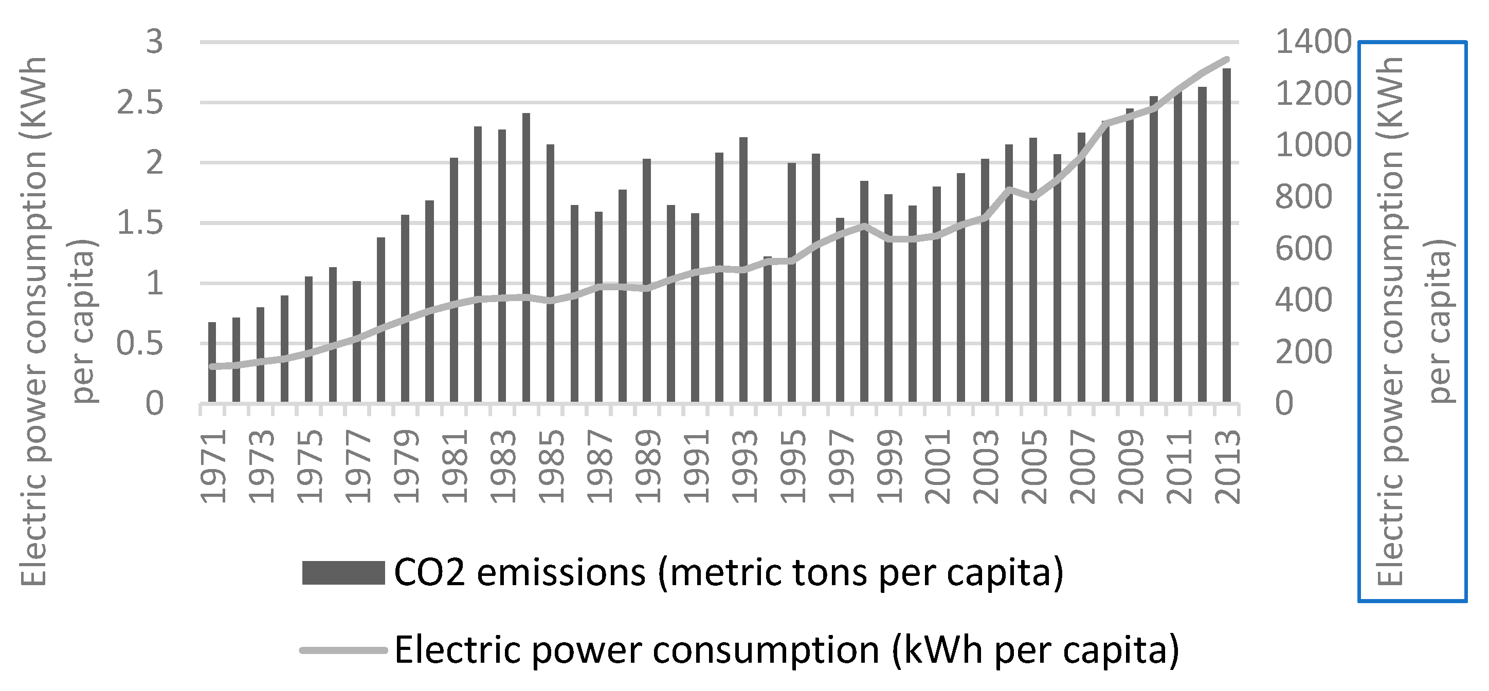
Figure 1. Relationship between CO2 emissions and electric power consumption in Ecuador. Source: Own elaboration based on data from the World Bank [43].
Sustainability 12 00853 g001
Figure 2. Relationship between CO2 emissions and provincial gross value added (GVA)—average 2007–2014. Source: Own elaboration, based on data from the provincial GVA of the Central Bank of Ecuador [53].
Sustainability 12 00853 g002
Figure 3. Aggregate value per capita (b) and provincial CO2 emissions (a) (tons per capita 2007 and 2014). Source: Own elaboration based on data from the Agency for Regulation and Control of Electricity and Ministry of Electricity and Renewable Energy [54] and the Central Bank of Ecuador [53].
Sustainability 12 00853 g003
Figure 4. Map of Ecuador.
Sustainability 12 00853 g004
Figure 5. Moran’s local and global index for the provincial CO2 emissions (tons per capita (a) 2007 and (b) 2014. Source: Own elaboration using the software GeoDa 1.14.0 (free and open source software tool, Loja, Ecuador).
Sustainability 12 00853 g005
Table 1. Study variables.
VariableDataSource of Information
CO2 emissions (tons)Energy consumption (MGW) by province (2007–2014).Annual and multi-year statistics for the Ecuadorian electricity sector. Agency for Regulation and Control of Electricity [54].
CO2 emission factor of Ecuador National Interconnected System for the years 2011, 2012 and 2013; and for the years from 2007 to 2010, the emission factor for 2011 was used.CO2 emission factor of Ecuador National Interconnected System.
Agency for Regulation and Control of Electricity and Ministry of Electricity and Renewable Energy [54] and the Central Bank of Ecuador [53].
Number of vehiclesNumber of motorized vehicles registered, according to provinces (2007–2014).Transportation statistics. Annual reports (2007 – 2014). National Institute of Statistics and Censuses [92].
Provincial Gross Added ValueGross Provincial Added Value (2007–2014).Provincial accounts 2007–2014. Central Bank of Ecuador [53].
Poverty due to incomeIncome poverty index (province) (2007–2014).Calculations from the Survey of employment, unemployment and underemployment, quarterly urban, period 2007–2014. National Institute of Statistics and Censuses [52,93,94].
Years of schoolingYears of Schooling (2007–2014).Years of Schooling by province, period 2007–2014. Integrated System of Social Indicators of Ecuador [95].
Gini coefficientGini coefficient, provincial (2007–2014).The regional inequality in Ecuador. Prepared based on national employment and unemployment surveys (ENEMDU) surveys [52,93,94].
Source: Own elaboration.
Table 2. Results of the panel models.
CO2Fixed EffectsRandom Effects
VEHICLESPC1.11091.0517
(5.69) (0.000)(5.25) (0.000)
GVAPC0.01340.0118
(4.72) (0.000)(4.30) (0.000)
GVAPC2−0.0002−0.0001
(−3.92) (0.000)(−3.65) (0.000)
GINI0.09760.1069
(0.86) (0.393)(0.90) (0.370)
SCH−0.0273-0.024
(−2.63) (0.009)(−2.30) (0.021)
PPI-0.0515−0.0987
(−0.70) (0.487)(−1.29) (0.196)
_cons0.41760.4138
(3.83) (0.000)(3.63) (0.000)
sigma_u0.15790.1135
sigma_e0.04320.0432
rho0.93020.8731
R20.4210.414
F for μ_i = 0
F (20, 135)54.17
n162162
CO2 = Carbon dioxide emissions per capita; GVAPC = gross value added per capita; GVAPC2 = gross value added per capita squared; VEHICLESPC = number of vehicles per capita; PPI = provincial poverty index; SCH = years of schooling by province; GINI = provincial GINI coefficient. Note: In statistical brackets t and its probability.
Table 3. Results of the panel spatial models.
CO2cSAR EFSACSEM EFSEM REGSRPESDM RESDM FE
VEHICLESPC1.21721.24051.77711.69411.71921.72532.05192.0716
(6.24) (0.000)(6.74) (0.000)(10.18) (0.000)(8.27) (0.000)(7.78) (0.000)(7.75) (0.000)(9.88) (0.000)(10.64) (0.000)
GVAPC0.01540.01660.01570.017660.01670.01670.01480.0159
(5.68) (0.000)(6.29) (0.000)(7.28) (0.000)(7.49) (0.000)(6.89) (0.000)(6.90) (0.000)(6.19) (0.000)(6.98) (0.000)
GVAPC2−0.0002−0.0002−0.0002−0.0002−0.0002−0.0002−0.0002−0.0002
(−4.94) (0.000)(−5.40) (0.000)(−6.41) (0.000)(−6.54) (0.000)(−6.06) (0.000)(−6.07) (0.000)(−5.32) (0.000)(−5.93) (0.000)
GINI−0.0093−0.0156−0.0138−0.0242−0.0329−0.0335−0.0479−0.0459
(−0.09) (0.930)(−0.16) (0.874)(−0.19) (0.852)(−0.29) (0.774)(−0.37) (0.714)(−0.37) (0.709)(−0.52) (0.606)(−0.53) (0.595)
SCH−0.0291−0.0311−0.0278−0.0355−0.0325−0.0325−0.0184−0.0209
(−2.82) (0.005)(−3.17) (0.002)(−3.02) (0.002)(−3.64) (0.000)(−0.89) (0.372)(−3.15) (0.002)(−1.79) (0.074)(−2.13) (0.033)
PPI0.00570.0319−0.0608−0.0314−0.0554−0.0566−0.0721−0.0523
(0.08) (0.936)(0.48) (0.631)(−1.19) (0.235)(−0.54) (0.592)(−0.89) (0.372)(−0.91) (0.363)(−1.10) (0.272)(−0.85) (0.394)
W VEHICLESPC −1.4171−1.442
(−4.24) (0.000)(−4.61) (0.000)
W GVAPC −0.0166−0.0196
(−2.76) (0.000)(−3.32) (0.001)
W GVAPC2 0.00020.0002
(−2.58) (0.010)(−3.16) (0.002)
W GINI 0.0011−0.0216
(−0.10) (0.994)(−0.15) (0.880)
W SCH 0.01910.022
(1.16) (0.247)(1.41) (0.158)
W PPI 0.16820.1619
(1.29) (0.196)(1.32) (0.187)
_cons 0.46390.46480.1678
(3.53) (0.000) (4.38) (0.000)(4.41) (0.000)(0.92) (0.355)
μ med 0.0871 0.473 0.1602
ρ0.11670.1331−0.4417 0.3620.4067
(1.22) (0.223)(1.42) (0.156)(−4.22) (0.000) (4.04) (0.000)(4.74) (0.000)
λ 0.69420.53380.55730.5597
(−10.96) (0.000)(5.83) (0.000)(5.71) (0.000)(5.72) (0.000)
ф −0.0746
(−0.25) (0.805)
n168168168168168168168168
CO2 = Carbon dioxide emissions per capita; GVAPC = gross value added per capita; GVAPC2 = gross value added per capita squared; VEHICLESPC = number of vehicles per capita; PPI = provincial poverty index; SCH = years of schooling by province; GINI = provincial GINI coefficient; SAR = Spatial auto regression model; SAC = Spatial simultaneous autoregressive model; SEM = Structural equation modeling; GSRPE = Generalized spatial panel random effects model; SDM = species distribution modelling. Note: In statistical brackets z and its probability. Source: Own elaboration based on regression results.
Table 4. Spatial Multipliers impact on CO2.
SDM RE
DirectIndirectTotals
VEHICLESPC1.9808***−0.9774**1.0034**
GVAPC0.0137***−0.0178**−0.0041
GVAPC2−0.0002***0.0002**0.0001
GINI−0.0491−0.0179−0.067
SCH−0.0150.01750.0025
PPI−0.04150.20750.166
SDM FE
DirectIndirectTotals
VEHICLESPC1.9981***−0.9099**1.0882**
GVAPC0.0145***−0.0215**−0.007
GVAPC2−0.0002***0.0003**0.0001
GINI−0.0514−0.0697−0.1211
SCH−0.01710.02210.005
PPI−0.02040.22220.2018
Significant * to 10%, ** to 5%, *** to 1%.