Informing Sustainable Consumption in Urban Districts: A Method for Transforming Household Expenditures into Physical Quantities

Abstract

Interventions targeted at district-level are a potentially effective way to reduce consumption-based urban impacts; however, a systematic method for accounting these impacts at district scale has not yet been developed. This article outlines a method for transforming household expenditure data into consumption quantified on a physical basis. Data sources are combined to calculate monetary value per unit mass for different products consumed by households. Socio-economic household archetypes are selected, and typical consumption for these archetypes is calculated by combining expenditure data from a household budget survey with the calculated monetary values per unit mass. The resulting physical quantities of different products consumed are envisaged as an essential part of performing district scale material flow analysis and urban metabolism studies, also as an input for assessing consumption-based environmental impacts and for designing sustainable consumption policies. The method was applied to characterise consumption in urban districts. The obtained results were used to assess of districts’ consumption-based impacts with life cycle assessment (LCA) and to inform design of sharing economy. The method was found to be an effective way to evaluate the demand for products in different districts; this in turn could inform objective measures to aid more sustainable urban consumption.

1. Introduction

From a life cycle perspective, it has been acknowledged that household consumption represents over three fifths of the environmental impact of total consumption and contributes the largest proportion of greenhouse gas (GHG) emissions from human activities [1,2]. In 2018, 55% of the global population lived in cities, a figure that is expected to increase to 70% by 2050 [3]. Aside from this, urban metabolism (UM) studies have shown that urban consumption is not only growing in absolute terms, but also per capita [4,5,6,7,8,9]. There is evident need for efforts to reduce the environmental impacts of household consumption, particularly as the growing human population increasingly shifts towards living in urban areas and adopting more consumerist lifestyles. Policies and measures addressing urban household consumption are a potentially effective mitigation strategy.

A number of methods have been used to investigate household consumption at urban scale. Lenzen and Peters used multi-regional input-output (MRIO) based on supply-use regional transaction tables in Sydney and Melbourne [10]. By supplementing the collated data with spatial detail derived from local land-use maps, pollution inventories and business registers, they were able to produce results comparable to having using life cycle analysis (LCA). In this case, industry and business transaction data from multiple sources was combined in spatial MRIO to characterise factors such as water use and GHG emissions at city level. The method cannot be easily adapted to different geographical regions and would be challenging to implement at district scale due to an inherent lack of industry in residential areas. Only one family archetype was made for each city, giving limited insight into household consumption as differences between households within the same city were not considered.

Miehe and colleagues used MRIO-LCA to study household carbon footprints (HCF) of German households, scaling data provided by individual households through expenditure surveys up to a regional level to give an overall average HCF comparison for different regions [2]. They found that there were large regional differences in HCF and proposed that considering household consumption at a localised rather than national scale would be more beneficial for developing effective and targeted emission reduction policies. The method is not applicable to different areas due to the development of 578 geographically specific household archetypes that are not valid in other contexts.

Jones and Kammen used IO-LCA combined with household budget survey (HBS) and census data for individual households to find average HCF for each US zip code. Again, differences between households in the same zip code are not accounted for as only an average is found [11]. Froemelt and colleagues used HBS data and combined it with existing models for building stocks, energy and transport to create a map of average per capita household GHG emissions for all municipalities in Switzerland [12]. Here, data from individual households was applied to municipal level. As this study offers a comprehensive and bottom-up model based on existing Swiss models and highly specific household archetypes, there is limited geographical applicability which would not be easy to replicate elsewhere.

Conversely, very small-scale studies have demonstrated that tailored solutions can be provided where a lot of detail is available. Greiff et al. studied sixteen households through surveys to calculate material and carbon footprints, Harder et al. illustrated methods for tracking masses of products in individual households consumption and waste generation through entries in an online system or smartphone [13], and Laakso and Lettenmeier applied MIPS (material input per unit of service) to five Finnish households [7,14]. In the study by Laakso and Lettenmeier, participating households positively changed their consumption behaviours as a result of engagement with the researchers and receiving household-specific information. However, potential environmental impact savings from so few households are limited and studies with this level of collaboration are unfeasible at a larger scale. Furthermore, information from small-scale studies cannot be extrapolated to approximate broader consumption patterns. Some authors identify that it is important to provide households with information that can help them make more environmentally responsible choices, but certain groups may need more support or even incentives to adopt more sustainable lifestyles [15,16].

With this in mind, identifying consumption patterns for particular household types and providing information or schemes accordingly could be an alternative way to encourage better consumption behaviours. The OECD report “Household Behaviour and the Environment—Reviewing the Evidence” suggests that policies should be targeted to account for differences in household types, but identifies that this may be costly to implement [15]. This may be more feasible if a low-cost method was available which could help ensure that both the right schemes and information were available to relevant households to assist them in making better decisions.

It is proposed that interventions at city scale could be an effective way to positively influence household consumption in urban areas. However, this may be challenging as cities tend to undergo continuous development, as well as having differences in land-use and high population heterogeneity [17,18]. Districts can be seen as urban areas with sufficient homogeneity to allow for straightforward and realistic household consumption estimations, and also large enough populations to support potentially impactful change [18]. As yet, district scale has rarely been addressed in UM studies and household consumption of goods has not previously been included [17,18,19]. The UM concept describes cities as complex systems that consume resources and produce waste and emissions in order to maintain their functions, much like an organism or ecosystem. Urban Metabolism studies apply material flow analysis and other methods to quantify types and masses of resources consumed, allowing reduction in resource use and consumption-based environmental impacts through monitoring and policy formulation. This approach can also provide decision-makers with quantitative analysis that identifies target product groups or can give indication of which policies might help to reach environmental goals [20,21,22]. To that end, local decision-makers may benefit from quantified insights into household consumption in a particular area that could inform more targeted initiatives.

Existing methods for studying household consumption tend not to be suitable for application at district level. The results are often geographically specific, expressed in monetary units and investigate specific environmental impacts. If the mass of goods can also be derived from monetary data, this would contribute to development of comprehensive district-scale UM accounting. It could also inform development of different schemes for reducing product consumption, in addition to broad impact evaluation. For this reason, a new method is outlined for quantifying household consumption on a mass basis. An example of how the method was applied to districts in the city of Gothenburg, Sweden, is presented to demonstrate that the method is effective at district-level. Application of data outputs from the method are illustrated with two policy-relevant examples: designing sharing economy and to aid in reducing consumption-based environmental impacts including climate change and acidification.

2. Materials and Methods

The developed method is based on the principle that quantifying household consumption on a mass basis offers flexibility for this data to be applied in different ways. Simple archetypes are formed that can be readily adapted to different geographical areas where household expenditure data is available. A diagram of the method developed in this study is presented in Figure 1. The method can be split into a four-step process, as outlined in the following sections. Socio-economic household archetypes should be set using parameters of interest available in the HBS, such as income and dwelling type. The first step in the method is focused on gathering and collating appropriate datasets. In the second step, the datasets are transformed into mass units to allow consumption per household archetype to be quantified to be defined in the third step. The final step extrapolates the household archetypes into spatial units.

2.1. Step 1—Data Collection

The main data source for this method is the HBS, sometimes called household expenditure survey, which provides expenditure data and associated socio-economic factors and is available in many countries. In this paper, the Swedish HBS from 2012 was used. The Swedish HBS is typically conducted at three year intervals, and Statistics Sweden (SCB) asks survey participants to record their spending on various products and services within a two-week period [23]. Additional data sources are required as HBS data does not generally include unit prices and masses for individual products. In this study, the consumer price index (CPI), conversion factors from Eurostat (ECF) and supplementary data from retail were used. Socio-economic characteristics (SEC) of households in the study area are needed to enable application of data outputs. In order to harmonise the various datasets used, correspondences between them were defined using standard nomenclature systems.

There are a number of different nomenclature systems used for coding and organising products that are traded, many of which have correspondence tables that are available through sources such as Eurostat RAMON [24]. In the Swedish HBS, expenditure was reported for products organised by COICOP codes (classification of individual consumption according to purpose) [25], without indication of the number of units purchased. To connect expenditure with product unit mass, unit prices were extracted from the Swedish CPI (consumer price index) and unit masses from ECF (conversion factors from Eurostat); product data for both is organised by combined nomenclature (CN) codes [26]. There was no existing equivalence between COICOP and CN, so a new correspondence was developed by linking existing tables with common nomenclature, as shown in

Table 1. Creating correspondence between COICOP nomenclature and CN nomenclature.

Primary Nomenclature	Secondary Nomenclature	Purpose in Method	Source
CN 2011	CPA 2002	Intermediate step for being able to link CN product mass data with COICOP expenditure data.	Eurostat RAMON
COICOP 1999	CPA 2002	Intermediate step for being able to link CN product mass data with COICOP expenditure data.	Eurostat RAMON
CN 2011	COICOP 1999	Links between CN product mass data and COICOP expenditure data.	Produced by combining CN 2011—CPA 2002 and COICOP 1999—CPA 2002 tables

. See S1 in the Supplementary Materials for the detailed correspondence.

2.2. Step 2—Data Transformation

The initial data transformation task was to remove services and intangible products from the HBS database. Following this, the HBS was further filtered to exclude products that were not part of the Swedish CPI for the same year as the HBS study. This was because household expenditure on goods was a fixed variable in this study, so it was important to work from a basis of product prices which were reflective of what households participating in the HBS would have paid. As the CPI offers a comprehensive overview of the prices for goods within a specified time frame and geographical region, it was assumed that using average product prices calculated from CPI data would provide consistency in subsequent calculations. The products where expenditure data and average unit price were available in the HBS and CPI databases respectively will be referred to as HBS-CPI products.

To obtain monetary value per unit mass of products, average unit prices and masses needed to be established for each product. For many products this was available in the CPI, however, for products not covered by CPI, price and mass data from other sources had to be combined. Many of the remaining product masses were available via ECF, and all other product masses were found through retail (as shown in Figure 1). Priority was given to CPI product masses, as these were for exactly the same products that were included in the average product prices. ECF was favoured over retail for the remaining product masses, as the ECF databases already had a large number of product masses collated by CN codes. S2 in the Supplementary Materials summarises the unit masses for products not commonly sold on a mass basis; S3 outlines the calculated kr/kg (where kr is Swedish crown) for different products and the sources of mass data.

Step 2a—Finding monetary value per unit mass from CPI data

The Swedish CPI product list was filtered to remove products which were not part of the HBS, using the developed correspondence between the COICOP codes used in HBS and CN codes used in CPI. Products where mass was reported alongside price were considered to be the most reliable. In some cases (especially for liquid products such as beverages), the products were instead reported on a volume basis which could then be converted to a mass (with the assumption that 1 litre of product had a mass of 1 kg).

For products where mass data was readily available within CPI, the mean mass per product was calculated, taking into account all products where the CN and COICOP codes matched. When product codes had multiple individual products attributed to them, all relevant product masses were included in the mean for each code. The monetary value per unit mass for each HBS product was then calculated using Equation (1), where standardised mass per unit is the unit of mass (e.g., 1 kg) divided by the mass of one product unit (e.g., the mass in kilograms of a single product).

$$\mathrm{Monetary}\mathrm{value}\mathrm{per}\mathrm{unit}\mathrm{mass}=\frac{\mathrm{average}\cos \mathrm{t}\mathrm{per}\mathrm{unit}}{\mathrm{standardised}\mathrm{mass}\mathrm{per}\mathrm{unit}}$$

(1)

Step 2b—Finding monetary value per unit mass from ITS data

The ECF database of product masses (available from Eurostat) was used to find mass per unit for products which were not recorded on a basis of physical units in CPI. Within the ECF database, products are described on a net mass basis along with supplementary units and are independent of price. However, the International Trade Statistics (ITS) database did not include masses for all of the products included in the HBS, so it was necessary to supplement the data with product masses from retail.

Step 2c—Finding monetary value per unit mass from retail data

For products that were not available in the CPI or ECF databases, masses were found from websites for retailers that are commonly used in Sweden. For example, homeware and furniture masses were taken from the IKEA website. One product weight was selected for each product listed in the HBS.

An exception to this is for personal vehicles, which can differ in price by several orders of magnitude despite having relatively similar masses. The mass of a car is also generally at least one order of magnitude greater than the mass of other products consumed by households, so it is necessary to adjust for this and prevent reported expenditure on cars introducing skew into the results. When looking at the expenditure data, the cars are noted as either purchased (1) or not purchased (0), using the assumption that households will only buy one car within a year. The proportion of households in each archetype that reported making a purchase is found, and then multiplied by the average mass of a car. This will give an adjusted number of kilograms consumed.

2.3. Step 3—Consumption Patterns

The next stage in the data transformation was to connect expenditure data together with monetary value per unit mass and combine this with socio-economic characteristics (SEC) to form typical consumption archetypes.

Step 3a—Converting HBS data from expenditure to physical units

The calculated monetary value per unit mass for HBS-CPI products were next combined with actual reported expenditure data from Swedish households. A database was created with kr/kg prices for the different products listed alongside the COICOP codes for each product. As the data in the HBS was confidential, this database was imported into the Statistics Sweden’s (SCB) secure system for working with microdata [27]. The household expenditure microdata and kr/kg pricing were combined using the statistical software R, using the COICOP codes to match the two datasets together. Reported household expenditure in kr was then divided by the kr/kg price for each product in order to give an estimate of the physical amount (in kg) of product that each individual family consumed.

Step 3b—Creating household archetypes

Pre-defined socio-economic archetypes based on parameters collected in the HBS were applied to enable analysis of consumption patterns for different household types. In this study, three simple filters were used to build the archetypes:

• Income—households were separated into different income groups based on quartile ranges for income in Sweden. Households in the first quartile were designated as low-income, the second and third quartiles were combined to give the middle-income group, and households in the fourth quartile were classed as high-income.
• Children—households were separated into those with children and those without.
• Dwelling type—households were separated into those living in multiple-occupancy dwellings (apartments) and those living in single-occupancy dwellings (houses).

Consumption patterns for each archetype were estimated by calculating the mean mass of each product type consumed by all households within the archetype.

2.4. Step 4—Data Outputs

The data outputs from the method are the estimated masses of different products consumed by households within the different archetypes. The archetype consumption patterns derived can be applied to any area with similar socio-economic characteristic data within the geographical bounds of the HBS that the method was used for.

The estimated masses consumed can be linked to environmental impact profiles. The kilogram of products consumed are multiplied by impact per kilogram (e.g., kg CO₂-eq), quantified from existing LCA data. The results can then be used to identify primary consumers of high-impact goods, and may even be coupled with geographical districts to find appropriate sharing schemes.

2.5. Assumptions and Limitations

A number of assumptions were needed to derive estimated household archetype consumption patterns using the developed method. One limitation is the accuracy of data obtained through HBS. In Sweden, the HBS is sent out to randomly selected households that need to complete an expenditure diary during a two-week period at a certain point within a year, plus telephone interviews about purchases of durable goods; different two-week periods are allocated to randomly selected households to account for seasonality in purchasing patterns [23]. The expenditure data quality is therefore reliant on the accuracy of reporting by members of the public.

Assumptions were required when developing nomenclature correspondence. For some products, particularly durable goods, there was no exact correspondence between COICOP and CN product descriptions. However, it was generally possible to cover the COICOP listed in the HBS by attributing multiple CN product codes to a single COICOP code, for example, CN 1412 (milk) was matched with both COICOP 01,141 (milk with fat content >1.5%) and COICOP 01,142 (milk with fat content <1.5%). For these products, it was assumed the average product mass for all relevant CN products could be used in combination with the average CPI price for all relevant CN products to give a representation monetary value per unit mass.

A further limitation was the quality of product mass data. The sequence filtering mass data gave priority to CPI (considered the most accurate due to availability of both product masses and prices), then ECF and lastly retail. Product codes where mass data had to be taken from retail tended to represent a number of different products; although the average mass per unit would not be reflective of any single item, the overall representation should be reasonable, particularly as the expenditure data did not clarify the exact products that had been purchased. It was assumed that the products in the average mass and average price calculations were sufficiently similar to give a fair comparison.

The broad archetypes developed from socio-economic factors with this method are widely applicable. However, using limited socio-economic variables to create the archetypes may have resulted in formation of heterogenous groups, due to potential variations between households within the same archetype. Furthermore, there were inequalities between the number of households in each archetype who participated in the Swedish HBS, meaning that some archetype consumption patterns are based on the mean data from a larger number of households than others. The data for the archetypes with more households in them may be more representative than for the smaller archetypes.

3. Results

3.1. Method Development

The method developed in this paper draws together data from different sources to enable the transformation of household expenditure data archetypal consumption patterns on a physical basis. This can be applied in different ways, as outlined in Section 3.2 and Section 3.3.

3.1.1. Data Transformation

The first part of this method required correspondence between different nomenclatures to be found in order to be able to connect data sets. The results from the 2012 Swedish HBS were used as a starting point; this was the most recently HBS published in Sweden. In total, 2871 households had participated, and socio-economic data for each anonymised household was presented alongside the expenditure that they had recorded for different products during the two-week survey period.

In order to convert the HBS expenditure data into physical units, it was necessary to connect product unit prices and masses from other sources to the expenditure reported by households.

Table 2. Number of products taken from different data sources.

Data Source	Description	Number of Products
HBS	Original product list (including services and intangibles)	835
HBS	Excluded from original product list (services and intangibles)	422
CPI	Tangible products from HBS with unit prices listed in CPI (i.e., products included in this study)	207
CPI	HBS-CPI products reported in CPI on a mass basis	84
ITS	HBS-CPI product masses taken from ITS	87
Retail	HBS-CPI product masses taken from retail sources	36

shows the number of products that were taken from different data sources. Although there were 835 different expenditure categories reported in the 2012 HBS, 422 of these represented services or products that were considered intangible within the scope of this study. Additionally, only products for which unit prices were listed in the 2012 Swedish CPI were included. This meant that only 207 of the products included in HBS were suitable to be included (listed in the Table 2 as HBS-CPI products). As outlined in Table 2 and Figure 1, a filtering hierarchy was applied when establishing unit mass for different products. The 77 HBS-CPI products reported on a mass basis in CPI were almost exclusively food and drink products. The 74 HBS-CPI products where unit masses were taken from ITS included clothing and common generic items such as furniture. Masses of the remaining 35 products that were sourced from retail tended to more specialist items that might not be owned by all households, such as recreational equipment. Overall, almost 90% of expenditure on goods reported in 2012 Swedish HBS was represented by the HBS-CPI products. Although it would be possible to incorporate the remaining products by identifying additional product prices from retail data, this was not considered necessary in this study as most of the expenditure reported in HBS was included. Furthermore, the intention of the study was primarily to outline the developed method and to connect consumption with sharing economy. It is possible that there might be better similarity between identified products covered by HBS and CPI in data from other geographies. It has been noted that the quality of HBS studies in some countries is better than that in Sweden, which would in turn yield more accurate results from this method. For example, in Switzerland (which has roughly half the population of Sweden), almost four times as many households participated in the most recent HBS compared to the Swedish HBS that this study was based on. Additionally, although the Swiss HBS also used a 2 week reporting period, there were supporting questions about ownership of a range of other durable products that might help gain a more accurate insight into typical consumption habits [28].

Once unit masses and prices had been collated, this data was transformed into the monetary value per unit mass (in this case kr/kg) for each HBS-CPI product. They were then combined with the reported expenditure from HBS to give estimated masses of products consumed by individual households. Priority was given to products included in the 2012 CPI to ensure the best possible correspondence with the 2012 HBS data. The output from this was a database of masses of products consumed by 2871 households, along with the socio-economic characteristics of each household. The masses of products consumed, combined with the household demographics, formed the basis for identifying patterns of archetype consumption that were the main output of applying this method to the Swedish HBS.

3.1.2. Archetypes

Consumption patterns for simple household archetypes were found. The rationale behind developing these simple archetypes was to allow consumption data to be combined with socio-economic data from other sources more easily (see Section 3.3). The method allows the archetypes to be readily customised.

Table 3. Archetypes used in this method and number of participating households from the 2012 Swedish HBS falling under each archetype. Legend for archetype codes: First letter refers to income (l = low, m = middle, h = high), middle letters refer to whether or not households have children (nk = no children, wk = with children) and the final letter refers to the dwelling type (h = house, a = apartment).

Archetype Code	Income	Children	House or Apartment?	Number of Households in HBS 2012 Falling under Archetype
l_nk_h	Low	No	House	77
l_wk_h	Low	Yes	House	27
l_nk_a	Low	No	Apartment	264
l_wk_a	Low	Yes	Apartment	50
m_nk_h	Middle	No	House	420
m_wk_h	Middle	Yes	House	341
m_nk_a	Middle	No	Apartment	462
m_wk_a	Middle	Yes	Apartment	365
h_nk_h	High	No	House	266
h_wk_h	High	Yes	House	367
h_nk_a	High	No	Apartment	141
h_wk_a	High	Yes	Apartment	90

summarises the archetypes developed as part of this method, including the number of participant households from the 2012 Swedish HBS falling under each archetype. The average mass consumed of every HBS-CPI product by all households in each archetype was calculated. SCB requires a minimum of five households to have contributed for data to be considered sufficiently confidential to be reported. As the smallest archetype contained 27 households, this criterion was comfortably met. The Swedish HBS data is scaled from the two-week reporting period up to annual expenditure for each household. This means that the data for individual households is not representative, however, combining the data from multiple households yields reasonable estimated consumption. The consumption per archetype for different HBS-CPI products can be found in S4 in the Supplementary Materials.

3.2. Consumption-Based Impacts

Once the masses of different products consumed in a certain area have been calculated, these can be input into environmental assessment tools to evaluate different consumption-based impacts. In this study, the impacts of shareable goods (identified as products in the HBS categories clothing, home goods, transport, and recreation) were evaluated using previously reported LCA data [29,30,31,32,33,34], providing information on the environmental impact per kilogram of product. The results presented are based on a limited selection of LCA profiles and therefore do not represent the impact of households comprehensively, but rather illustrate possible results from the method. In line with previous studies, high-income households with children, living in houses had the highest environmental impact, regardless of impact type (see

Table 4. HBS-based environmental impacts per household archetype.

Household Type	Climate Change (kg CO2-eq)	Acidification (kg SO2-eq)	Photochemical Ozone Formation Potentials (kg C2H4-eq)	Eutrophication (kg PO43-eq)
l_nk_h	3223	20.8	0.01	0.06
l_wk_h	3525	20.4	0.12	0.14
l_nk_a	2143	12.0	0.08	0.14
l_wk_a	3180	18.5	0.11	0.13
m_nk_h	5547	34.8	0.07	0.18
m_wk_h	8288	51.0	0.14	0.29
m_nk_a	4760	30.2	0.05	0.25
m_wk_a	5794	33.0	0.20	0.34
h_nk_h	7143	43.9	0.13	0.38
h_wk_h	9494	54.9	0.31	0.51
h_nk_a	5525	34.8	0.06	0.30
h_wk_a	4638	27.2	0.15	0.37

) [35,36]. This would indicate that from an environmental impact perspective, encouraging high-income house dwellers and middle-income house-dwellers with children to engage in sharing economy would result in the greatest environmental impact reduction. The concept of sharing economy is that individuals have access to products and spaces rather than owning them; for example, a pool of users could share a product that might otherwise be an under-utilised private asset. This is intended to reduce the need for privately-owned goods, thus allowing people to adopt more “low-consumption lifestyles” [37]. Sharing economy is part of circular economy, a strategy which aims to maximise use of anthropogenic material stock in order to reduce waste, environmental impacts and demand for virgin raw materials [38].

The results can also be analysed by product group. Whilst transport had the highest impact for climate change, clothing and home goods drove acidification, and eutrophication effects were largest for home goods. There were limited profiles that included photochemical ozone creation potential, but again, clothing was a driver. Based on these findings, consumption of clothing and home goods should also be targeted in order to achieve reduction in environmental impacts. The results emphasise that to identify the product types with the most potential for impact reduction, it is important to investigate multiple indicators as opposed to focusing on a single measure such as climate change.

3.3. Sharing Economy

Considering the masses of shareable products consumed in different districts can also be useful in the design of sharing economy schemes. As shown in Figure 2, understanding the consumption patterns of different types of households enables commonly consumed products within a particular area to be identified. This enables localised schemes to be targeted either towards reducing consumption of particular goods for environmental sustainability, or to create social sustainability by providing access to products which may be widely consumed in wealthier districts but not in predominantly low-income areas. The districts shown in Figure 2 represent are comparable in size and dwelling type, but with different demographics. District A has 3245 low-income households, living in apartments. Almost half of these households have children. District B has 3221 middle-income households, who also live in apartments. Only 15% of the households in District B have children. Although the number of households in these two districts is almost identical, there are differences in the quantities and types of products consumed. Understanding the consumption habits of types of households in these districts would be beneficial for creating targeted schemes. Considering the product consumption shown in Figure 2, a potentially beneficial sharing scheme might be a toy library in District A. Comparing these two districts suggests that the consumption of toys and hobby products is almost 50% higher in District A than District B, but as there are 2.3 times more households with children in District A, this suggests that children in District A have access to fewer toys than those in District B. A toy library in District A would provide opportunities for children there to borrow toys that their families might not buy for them, which in turn might reduce social inequalities between children living in Districts A and B.

It is also possible to compare the environmental impact of districts by coupling the relevant consumption quantities to the environmental impacts.

Table 5. HBS-based environmental impacts per district.

Product Category	Climate Change (kg CO2-eq)	Acidification (kg SO2-eq)	Photochemical Ozone Formation Potentials (kg C2H4-eq)	Eutrophication (kg PO43-eq)
District A
Toys and hobby	109.0 × 104	996	236	95
Books	1.2 × 104	68	--	--
Bicycles	2.3 × 104	8	--	2.3
Clothing and footwear	57 × 104	2887	163	524
Cars	7468 × 104	49,457	--	--
Tools	58 × 104	--	--	--
Total impact	9745 × 104	53530	398	621
Total impact per household	2969	16	0.12	0.19
District B
Toys and hobby	73 × 104	669	158	63
Books	1.2 × 104	67	--	--
Bicycles	0.51 × 104	18	--	5
Clothing and footwear	68 × 104	3483	196	633
Cars	14,488 × 104	95,948	--	--
Tools	75 × 104	--	--	--
Total impact	1671 × 104	100435	354	701
Total impact per household	5110	30	0.11	0.21

-- impact type for which LCA data was not available.

presents a summary of four different impact types for shareable products in Districts A and B. Using the calculated consumption values for the districts described above, it was found that the overall environmental impacts per household in District B were nearly double those of District A when considering the products for which LCA profiles had been gathered. Both districts show cars as the product type with the greatest contribution. The next-highest contributing consumption category (i.e., toys and hobby, tools) differs between the districts, as do the relative contribution of each product category to the overall impact. These patterns in each districts’ consumption can inform development of district-specific policies that would satisfy the needs of residents while also promoting low-impact lifestyles. In this case, both districts could reduce their impacts by sharing toys, clothing, tools, and cars and motorcycles. Local consumption patterns could be used to design measures that strategically address environmental impact reduction from identified products. For example, our findings suggest that District A would achieve greater reductions than District B through implementing initiatives such as bicycle pooling or a “bicycle kitchen” where residents can access guidance and tools for repairs. This could even help reduce the impact from cars if it leads to a modal shift by residents. It should be noted that in the data used for this study, the HBS product category for “tools” also included non-shareable goods such as lightbulbs and batteries. Consumption data may therefore be over-estimated, with possible subsequent over-estimation of environmental impacts.

4. Discussion

The method proposed in this paper offers a simple way for local policy-makers to be able to assess the impacts of household consumption within a specific area. Existing methods for evaluating household consumption do not address consumption at district level, even though this resolution has been identified as having potential for positive environmental impact through targeted localised schemes [2]. Results from the method can be used to inform design of such localised policies with high potential engagement based on the needs of local people, both in terms of reducing the impacts of consumption in wealthier areas and improving access to goods for lower-income residents. This study proposes methodological advances by addressing the issue of combining monetary and physical data, which has been raised as a challenge in other studies [10]. Additionally, as this method quantifies physical flows of goods consumed by households within a geographical area, it can contribute to accounting district-scale MFA and study of neighbourhood-scale urban metabolism.

By innovatively combining two datasets that are commonly compiled by national statistical offices (HBS and CPI), the method developed in this study derives product cost per kg from unit price and mass. Extraction of data from additional sources was kept to a minimum to ensure that the method would be easily replicable without the need for specialist knowledge, or significant investment of time or money. Furthermore, the chosen socio-economic characteristics are applicable to different geographies and the household archetypes that have been created can help local decision-makers in cities (or even individual districts) to be better informed about household consumption impacts within their sphere of influence.

As the criteria for creating archetypes within this method is very simple, especially compared to other archetype-based studies [12,39], similar criteria for identifying patterns of archetype consumption could be applied to HBS data from other countries. Moreover, archetypes can be easily customised to be appropriate to specific areas of interest, within the limits of the socio-economic parameters of HBS. Froemelt and colleagues also used archetypes in their study of Swiss household consumption, but were unsure whether the 578 geographically-specific archetypes they developed would be transferrable to other regions [12]. The method outlined in this study can be easily applied in different contexts provided that the upper and lower income quartiles are known, so that the household incomes for the archetypes can be categorised as low, middle and high according to local economic conditions. Furthermore, the list of product unit masses compiled in this study would be suitable for combining with HBS and CPI data from other countries to apply this method to other geographies.

Whilst this study is not alone in scaling up consumption from individual households to urban-level [2,11,12], most other studies directly apply scaled data to calculate average HCF or GHG emissions per capita. Our proposed method gives consumption of specific products in physical terms, offering greater flexibility to apply the data in different environmental impact models, as illustrated in this study by estimation of four different impacts using LCA. This also allows evaluation of impacts from products of particular interest, rather than broad average impacts from all consumption as in other studies. Additionally, our method can be used to quantify physical flows of goods consumed by households within a geographical area. These quantified flows are purely reflective of private household consumption, unlike in other methods which tend to use MRIO and therefore derive household consumption from trade and industry flows. Furthermore, because the consumption patterns for different areas generated using our method are based on archetypes, the socio-economic characteristics of consumption reflect each area considered, enabling comparison between districts, including patterns of consumption for individual products in each area. This would be much more difficult to capture with MRIO.

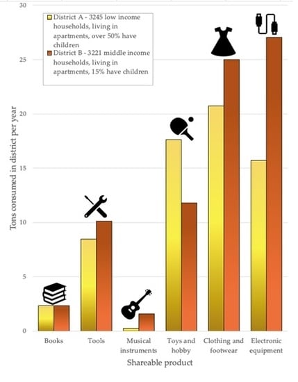
With regard to sharing economy applications, this method offers a straightforward way to evaluate or predict household consumption of products for a specific area. With unique potential for district-scale, this method can be used to identify hotspot districts with high consumption, or districts where consumption of specific products are high. Conversely, districts where residents are resource-poor relative to other areas could be identified. In turn, this can inform the design of localised sharing economy schemes at a district level, for both environmental and social sustainability. This is proposed as an effective approach due to the physical characteristics of particular districts and the tendency for socio-economic similarities between resident of the same district.

This study resulted in the initiation of a project in the city of Gothenburg. It is proposed that Gothenburg could be used as a test-bed for investigating practical applications of this method in more detail, as well as developing it further. Suggestions include quantifying the environmental and economic benefits of sharing economy (for the entire city, districts or of specific initiatives), identifying target districts or household types based on their consumption patterns, or developing customised initiatives for different household types. A case study has been proposed on a new district that currently being planned for development in Gothenburg. The purpose of the case study would be to create a specific plan for partially substituting product demand from households in the new district with shared products, based on the predicted distribution of household types.

References

1. Hertwich, E.G.; van der Voet, E.; Tukker, A. Assessing the Environmental Impacts of Consumption and Production. In Priority Products and Materials; United Nations Environment Programme: Nairobi, Kenya, 2010; ISBN 9789280730845. [Google Scholar]
2. Miehe, R.; Scheumann, R.; Jones, C.M.; Kammen, D.M.; Finkbeiner, M. Regional carbon footprints of households: A German case study. Environ. Dev. Sustain. 2016, 18, 577–591. [Google Scholar] [CrossRef] [Green Version]
3. United Nations World Urbanization Prospects: The 2018 Revision, Key Facts; United Nations: New York, NY, USA, 2018.
4. Kalmykova, Y.; Rosado, L.; Patrício, J. Resource consumption drivers and pathways to reduction: Economy, policy and lifestyle impact on material flows at the national and urban scale. J. Clean. Prod. 2016, 132, 70–80. [Google Scholar] [CrossRef] [Green Version]
5. Kalmykova, Y.; Rosado, L.; Patrício, J. Urban Economies Resource Productivity and Decoupling: Metabolism Trends of 1996–2011 in Sweden, Stockholm, and Gothenburg. Environ. Sci. Technol. 2015, 49, 8815–8823. [Google Scholar] [CrossRef]
6. Rosado, L.; Kalmykova, Y.; Patrício, J. Urban metabolism profiles. An empirical analysis of the material flow characteristics of three metropolitan areas in Sweden. J. Clean. Prod. 2016, 126, 1–12. [Google Scholar] [CrossRef]
7. Laakso, S.; Lettenmeier, M. Household-level transition methodology towards sustainable material footprints. J. Clean. Prod. 2016, 132, 184–191. [Google Scholar] [CrossRef] [Green Version]
8. Mont, O.; Neuvonen, A.; Lähteenoja, S. Sustainable lifestyles 2050: Stakeholder visions, emerging practices and future research. J. Clean. Prod. 2014, 63, 24–32. [Google Scholar] [CrossRef]
9. Lavers, A.; Kalmykova, Y.; Rosado, L.; Oliveira, F.; Laurenti, R. Selecting representative products for quantifying environmental impacts of consumption in urban areas. J. Clean. Prod. 2017, 162, 34–44. [Google Scholar] [CrossRef]
10. Lenzen, M.; Peters, G.M. How City Dwellers Affect Their Resource Hinterland. J. Ind. Ecol. 2010, 14, 73–90. [Google Scholar] [CrossRef]
11. Jones, C.; Kammen, D.M. Spatial Distribution of U.S. Household Carbon Footprints Reveals Suburbanization Undermines Greenhouse Gas Benefits of Urban Population Density. Environ. Sci. Technol. 2013, 48, 895–902. [Google Scholar] [CrossRef]
12. Froemelt, A.; Buffat, R.; Heeren, N.; Hellweg, S. Assessing environmental impacts of individual households: A large-scale bottom-up LCA-model for Switzerland. Abstr. B 2018, 147, 32–33. [Google Scholar]
13. Harder, R.; Kalmykova, Y.; Morrison, G.M.; Feng, F.; Mangold, M.; Dahlén, L. Quantification of Goods Purchases and Waste Generation at the Level of Individual Households. J. Ind. Ecol. 2014, 18, 227–241. [Google Scholar] [CrossRef]
14. Greiff, K.; Teubler, J.; Baedeker, C.; Liedtke, C.; Rohn, H. Material and Carbon Footprint of Household Activities. In Living Labs: Design and Assessment of Sustainable Living; Keyson, D.V., Guerra-Santin, O., Lockton, D., Eds.; Springer International Publishing: Berlin/Heidelberg, Germany, 2017; pp. 259–275. [Google Scholar]
15. OECD. Household Behaviour and the Environment-Reviewing the Evidence. Available online: https://www.oecd.org/environment/consumption-innovation/42183878.pdf (accessed on 21 January 2020).
16. Teubler, J.; Buhl, J.; Lettenmeier, M.; Greiff, K.; Liedtke, C. A Household’s Burden-The Embodied Resource Use of Household Equipment in Germany. Ecol. Econ. 2018, 146, 96–105. [Google Scholar] [CrossRef] [Green Version]
17. Codoban, N.; Kennedy, C.A. Metabolism of neighborhoods. J. Urban. Plan. Dev. 2008, 134, 21–31. [Google Scholar] [CrossRef]
18. Rosado, L.; Hagy, S.; Kalmykova, Y.; Morrison, G.; Ostermeyer, Y. A living lab co-creation environment exemplifying Factor 10 improvements in a city district. J. Urban. Regen. Renew. 2015, 8, 171–185. [Google Scholar]
19. Gontia, P.; Nägeli, C.; Rosado, L.; Kalmykova, Y.; Österbring, M. Material-intensity database of residential buildings: A case-study of Sweden in the international context. Resour. Conserv. Recycl. 2018, 130, 228–239. [Google Scholar] [CrossRef]
20. Lavers Westin, A.; Kalmykova, Y.; Rosado, L.; Oliveira, F.; Laurenti, R.; Rydberg, T. Combining material flow analysis with life cycle assessment to identify environmental hotspots of urban consumption. J. Clean. Prod. 2019, 226, 526–539. [Google Scholar] [CrossRef]
21. Lavers Westin, A.; Kalmykova, Y.; Rosado, L. Method for Quantitative Evaluation of Sustainability Measures: A Systems Approach for Policy Prioritization. Sustainability 2019, 11, 734. [Google Scholar] [CrossRef] [Green Version]
22. Brunner, P.H.; Rechberger, H. Practical Handbook of Material Flow Analysis; CRC Press: Boca Raton, FL, USA, 2016; ISBN 9780203507209. [Google Scholar]
23. Hushållens utgifter (HUT). Available online: https://www.scb.se/contentassets/90c71dbdb84c4fb5abb66896f3a478e6/he0201_do_2012.pdf (accessed on 19 November 2019).
24. European Commission Europa-RAMON. Available online: https://ec.europa.eu/eurostat/ramon/index.cfm?TargetUrl=DSP_PUB_WELC (accessed on 23 October 2019).
25. United Nations COICOP: Classification of Individual Consumption According to Purpose; United Nations: New York, NY, USA, 2018; Volume M.
26. European Commission. The Combined Nomenclature. Available online: https://trade.ec.europa.eu/tradehelp/eu-product-classification-system (accessed on 21 January 2020).
27. SCB MONA—A System for Delivering Microdata. Available online: https://www.scb.se/en/services/guidance-for-researchers-and-universities/mona--a-system-for-delivering-microdata/ (accessed on 21 January 2020).
28. Froemelt, A.; Dürrenmatt, D.J.; Hellweg, S. Using Data Mining to Assess Environmental Impacts of Household Consumption Behaviors. Environ. Sci. Technol. 2018, 52, 8467–8478. [Google Scholar] [CrossRef]
29. Cotton Incorporated. The Life Cycle Inventory & Life Cycle Assessment of Cotton Fiber & Fabric v2; Cotton Incorporated: Cary, NC, USA, 2012. [Google Scholar]
30. WRAP. Environmental Assessment of Consumer Electronic Products a Review of High. Volume Consumer Electrical Products through; WRAP: Banbury, Oxon, UK, 2010. [Google Scholar]
31. Liljenroth, U.; Eriksson, M. PM: Miljöeffekter av Delningsekonomi; WSP: Gothenburg, Sweden, 2018. [Google Scholar]
32. Naicker, V.; Cohen, B. A life cycle assessment of e-books and printed books in South Africa. J. Energy South. Afr. 2016, 27, 68–77. [Google Scholar] [CrossRef]
33. Hedman, E.A. Comparative Life Cycle Assessment of Jeans-A case study performed at Nudie Jeans. MSc thesis, KTH, Stockholm, Sweden, 2018. [Google Scholar]
34. EPD International AB EPD Search—The International EPD® System. Available online: https://www.environdec.com (accessed on 21 January 2020).
35. Heinonen, J.; Junnila, S. A carbon consumption comparison of rural and urban lifestyles. Sustainability 2011, 3, 1234–1249. [Google Scholar] [CrossRef] [Green Version]
36. Wier, M.; Lenzen, M.; Munksgaard, J.; Smed, S. Effects of Household Consumption Patterns on CO2 Requirements. Econ. Syst. Res. 2001, 133, 259–274. [Google Scholar] [CrossRef]
37. Eckelman, M.; Kalmykova, Y. Sharing and Environmental Sustainability. In SHARE: Engineering Sharing; Cambridge Press: Cambridge, UK, 2020. [Google Scholar]
38. Kalmykova, Y.; Sadagopan, M.; Rosado, L. Circular economy—From review of theories and practices to development of implementation tools. Resour. Conserv. Recycl. 2018, 135, 190–201. [Google Scholar] [CrossRef]
39. Baiocchi, G.; Minx, J.; Hubacek, K. The Impact of social factors and consumer behavior on carbon dioxide emissions in the United Kingdom. J. Ind. Ecol. 2010, 14, 50–72. [Google Scholar] [CrossRef]
Figure 1. Overview for method. Legend: HBS—household budget survey; COICOP—classification of individual consumption according to purpose; CPI—consumer price index; ECF—conversion factors from eurostat; CN—combined nomenclature; SEC—socio-economic characteristics.
Sustainability 12 00802 g001
Figure 2. Consumption of shareable products in two Gothenburg districts.
Sustainability 12 00802 g002