A Hybrid Intelligence Approach to Enhance the Prediction Accuracy of Local Scour Depth at Complex Bridge Piers

 ,
,  ,
,  ,
,  ,
,  ,
,  , ,
, ,
Abstract

1. Introduction
2. Methodology
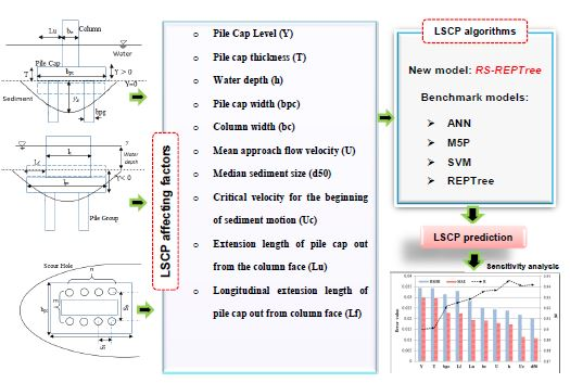
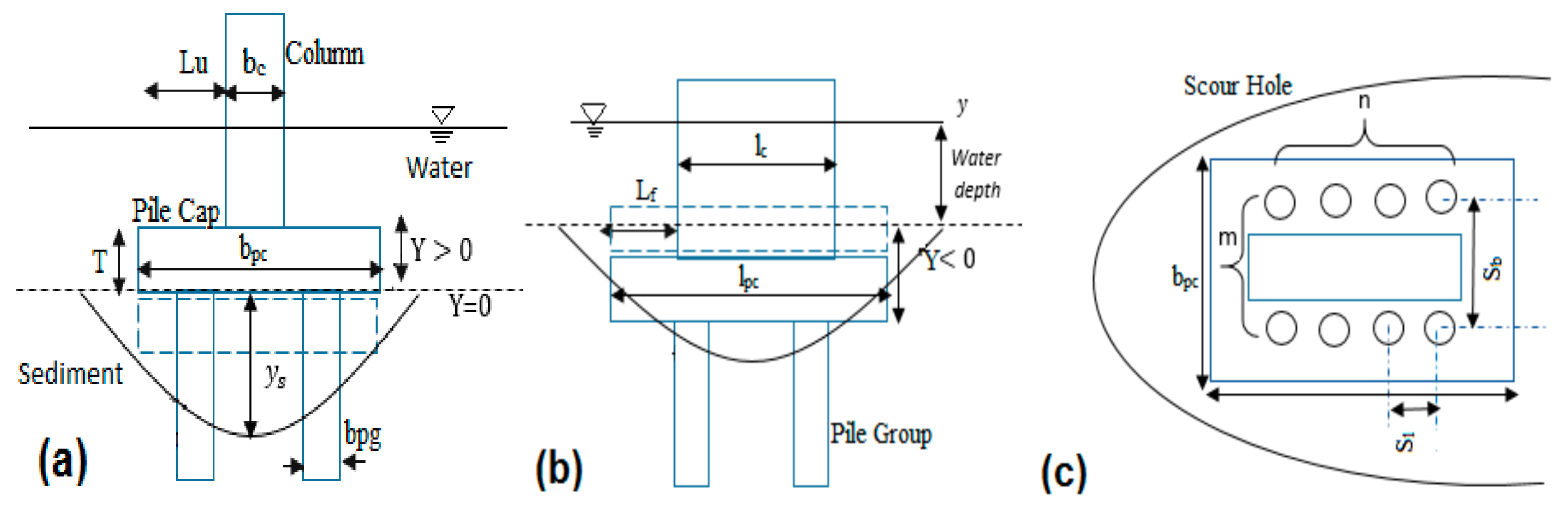
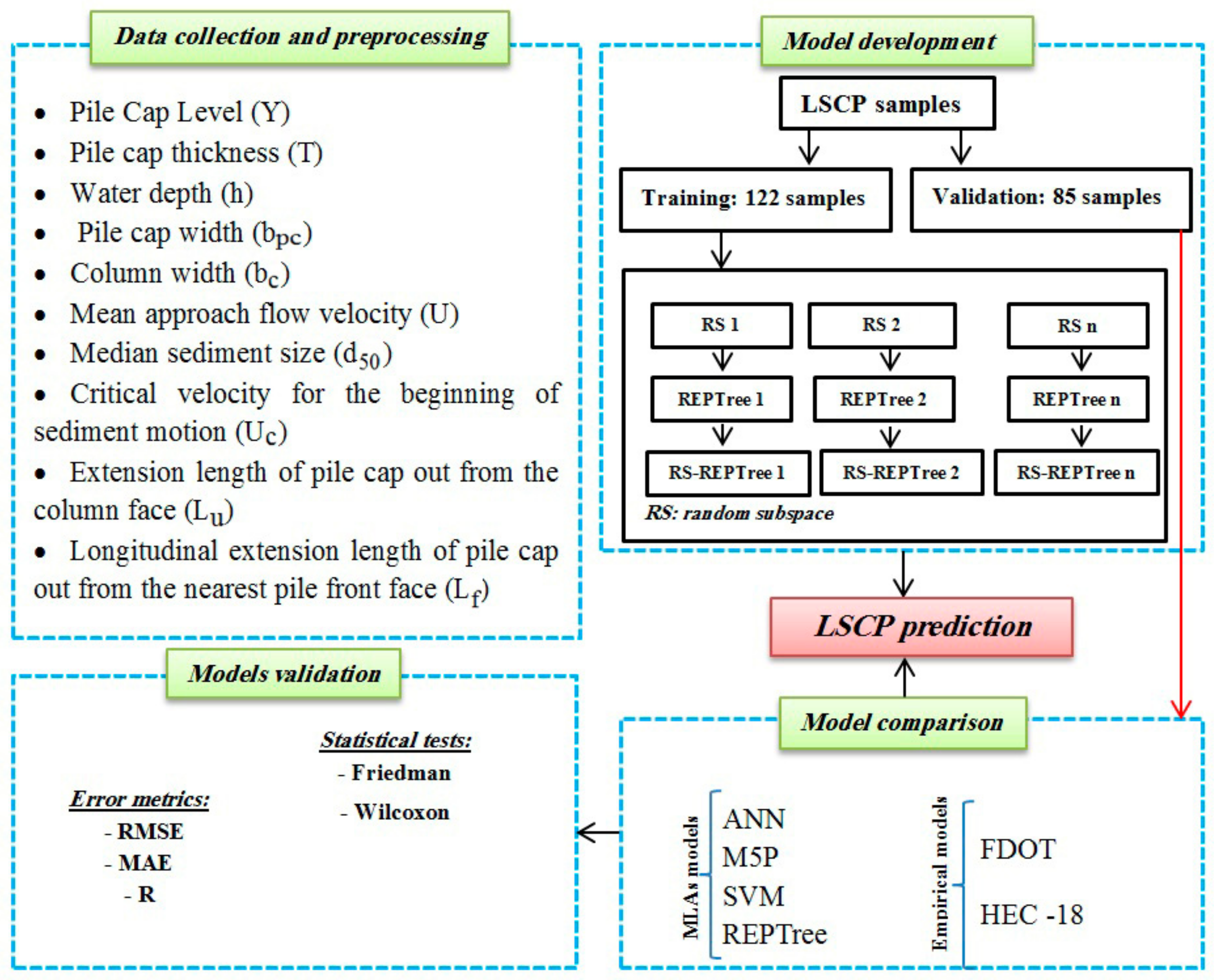
2.1. Data Acquisition
2.2. Dimensional Analysis
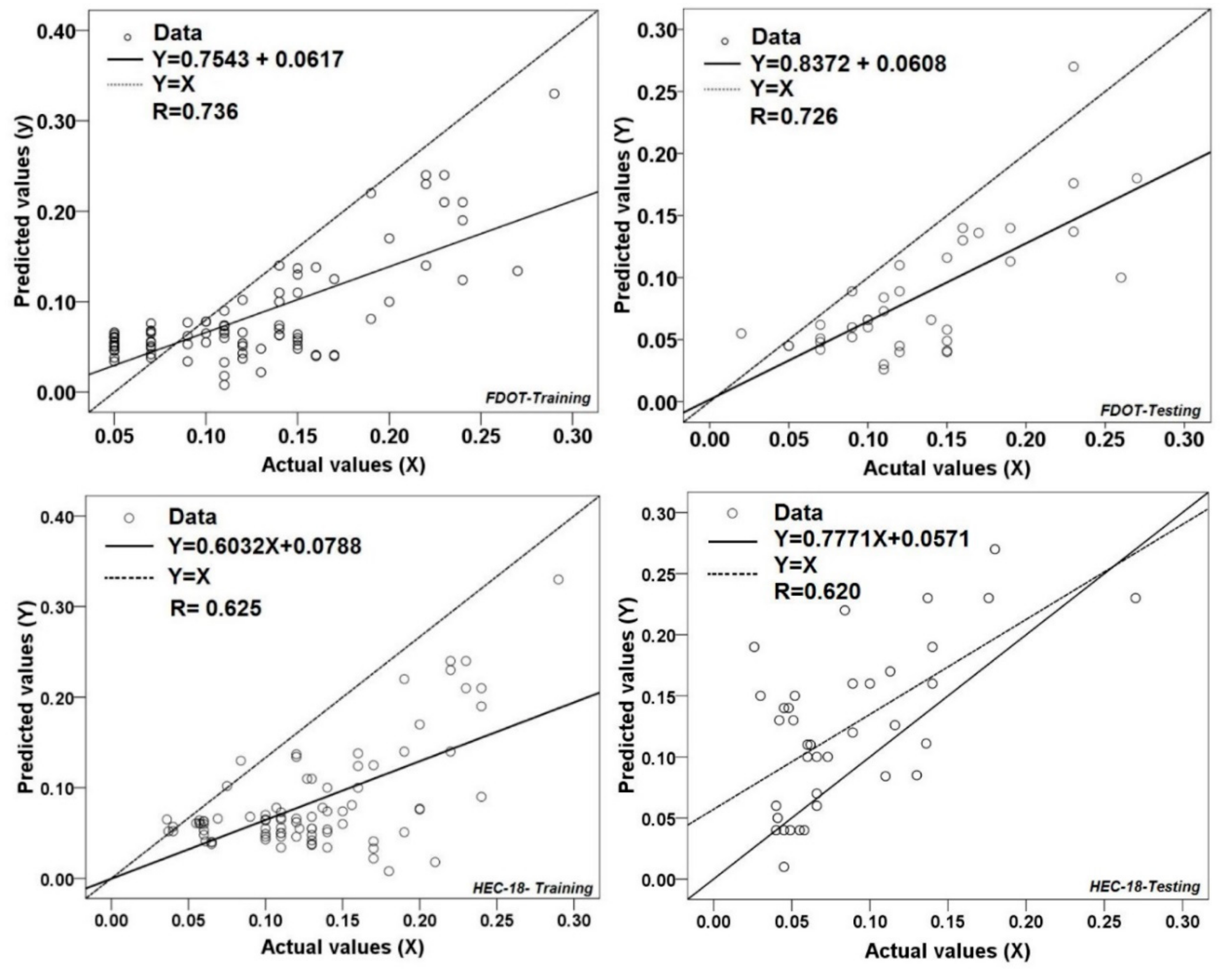
2.3. Empirical Equations
2.4. Machine Learning Algorithms
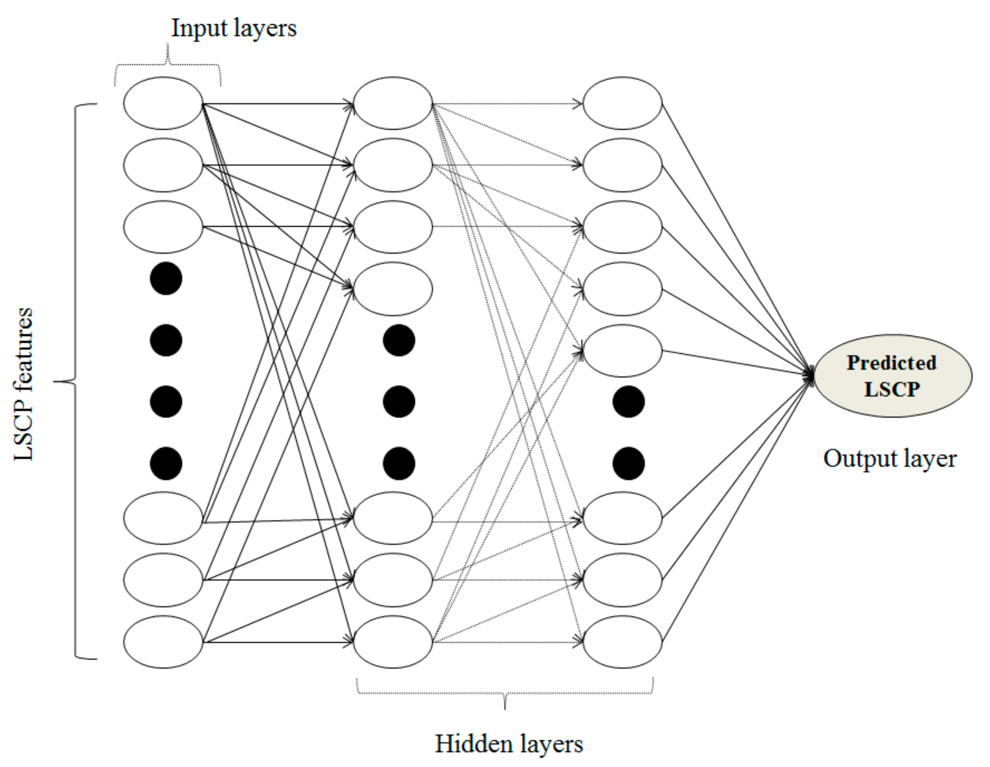
2.4.1. Artificial Neural Networks
2.4.2. M5P Model Tree
2.4.3. Support Vector Machine
2.4.4. REP Tree
2.4.5. Random Subspace Ensemble Algorithm
2.5. Evaluation and Comparison
2.5.1. Statistical Metrics
2.5.2. Non-Parametric Statistical Tests
2.6. Sensitivity Analysis
3. Results and Analysis
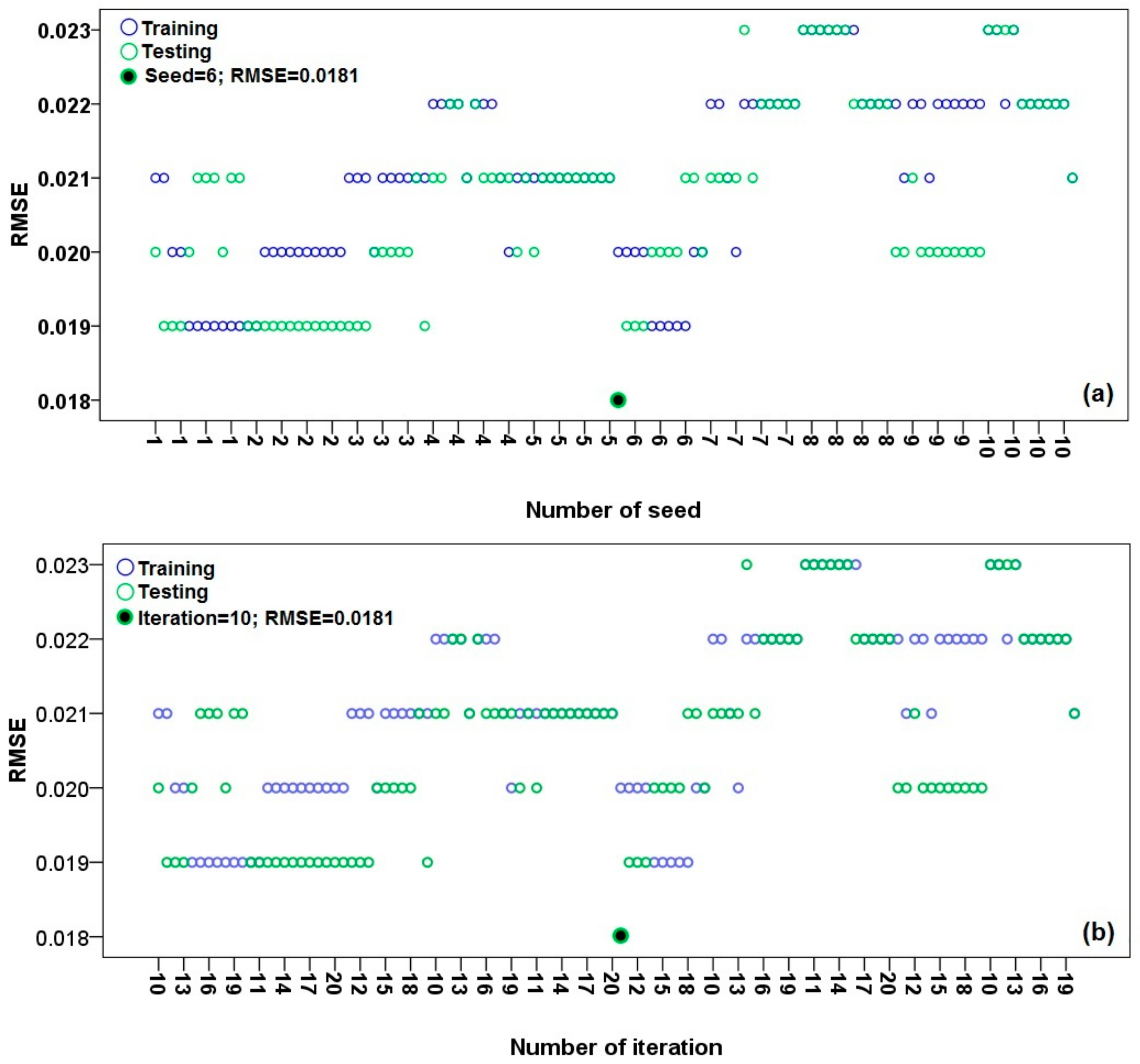
3.1. Optimal Selection of Modeling Parameters
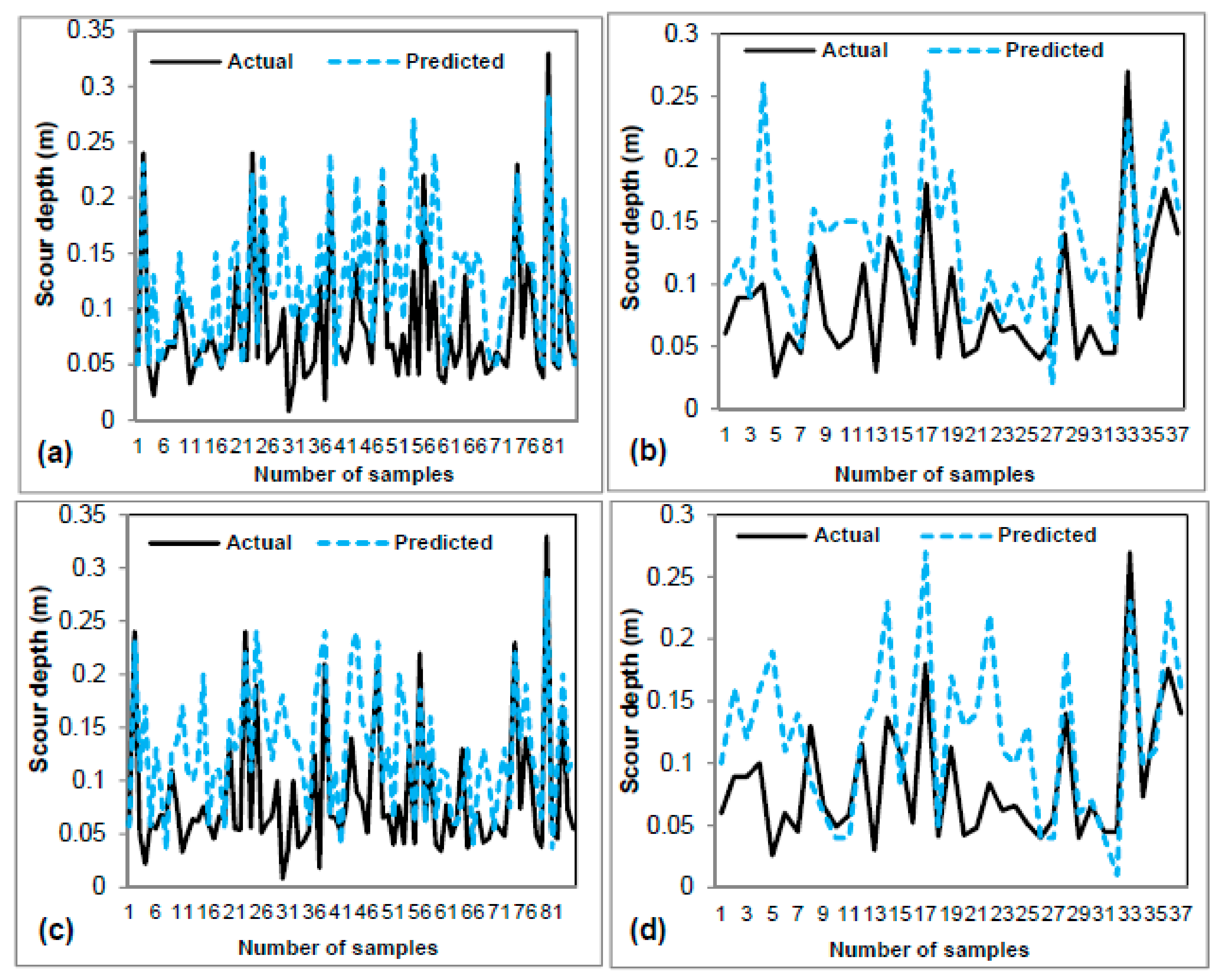
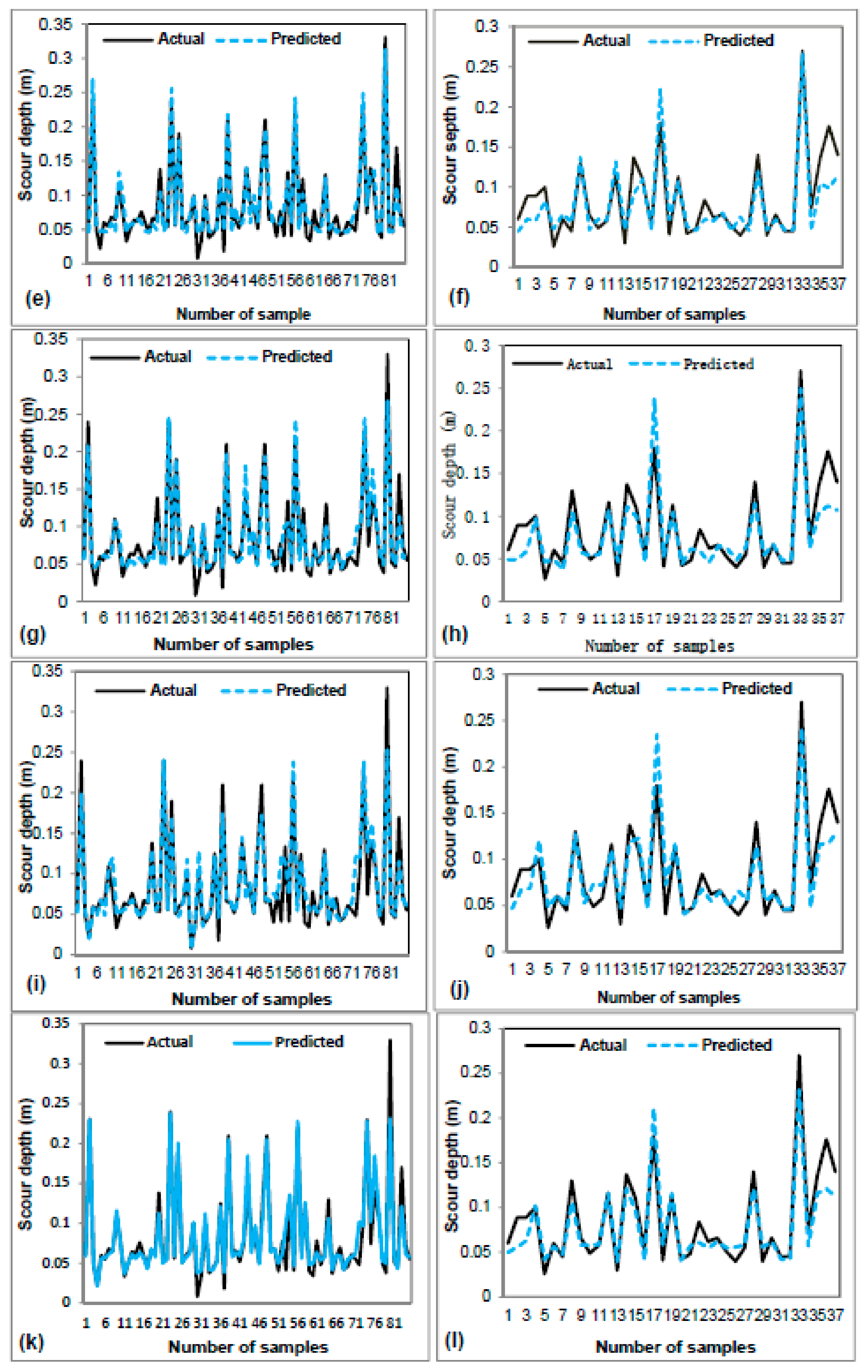
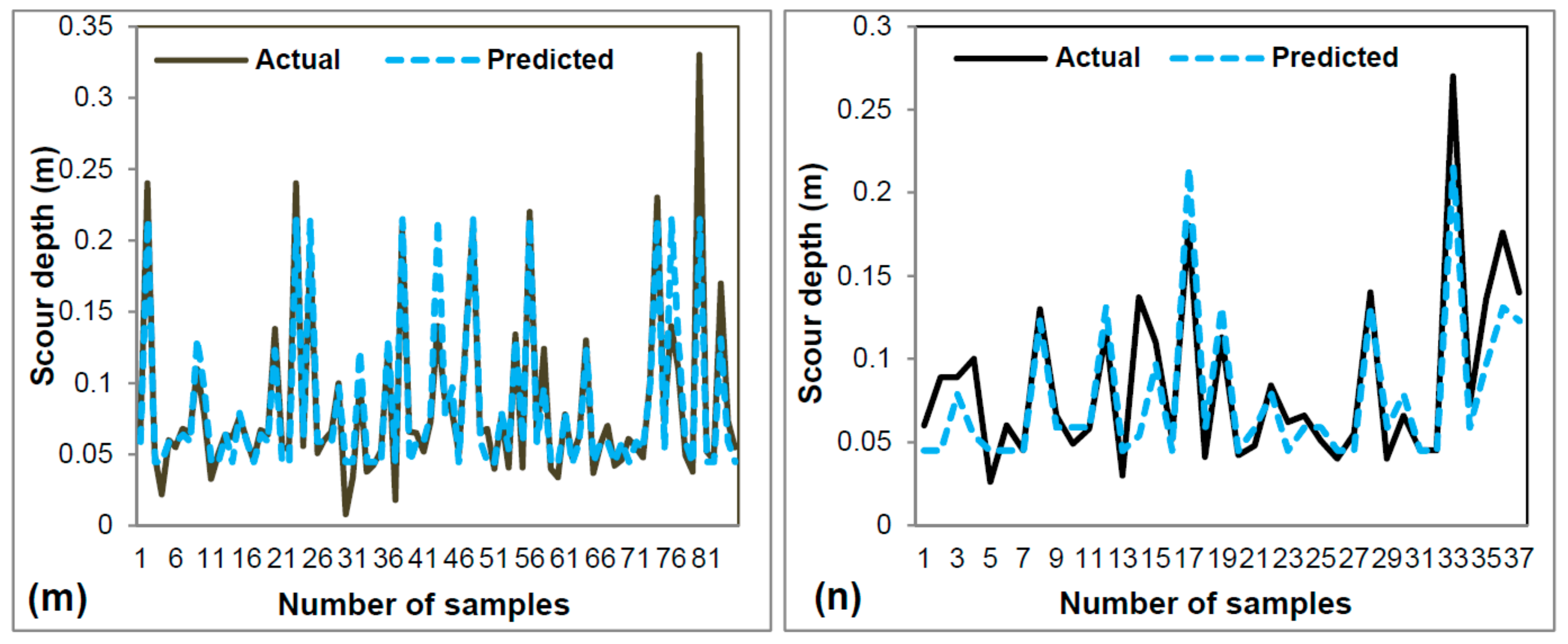
3.2. Model Validation and Comparison
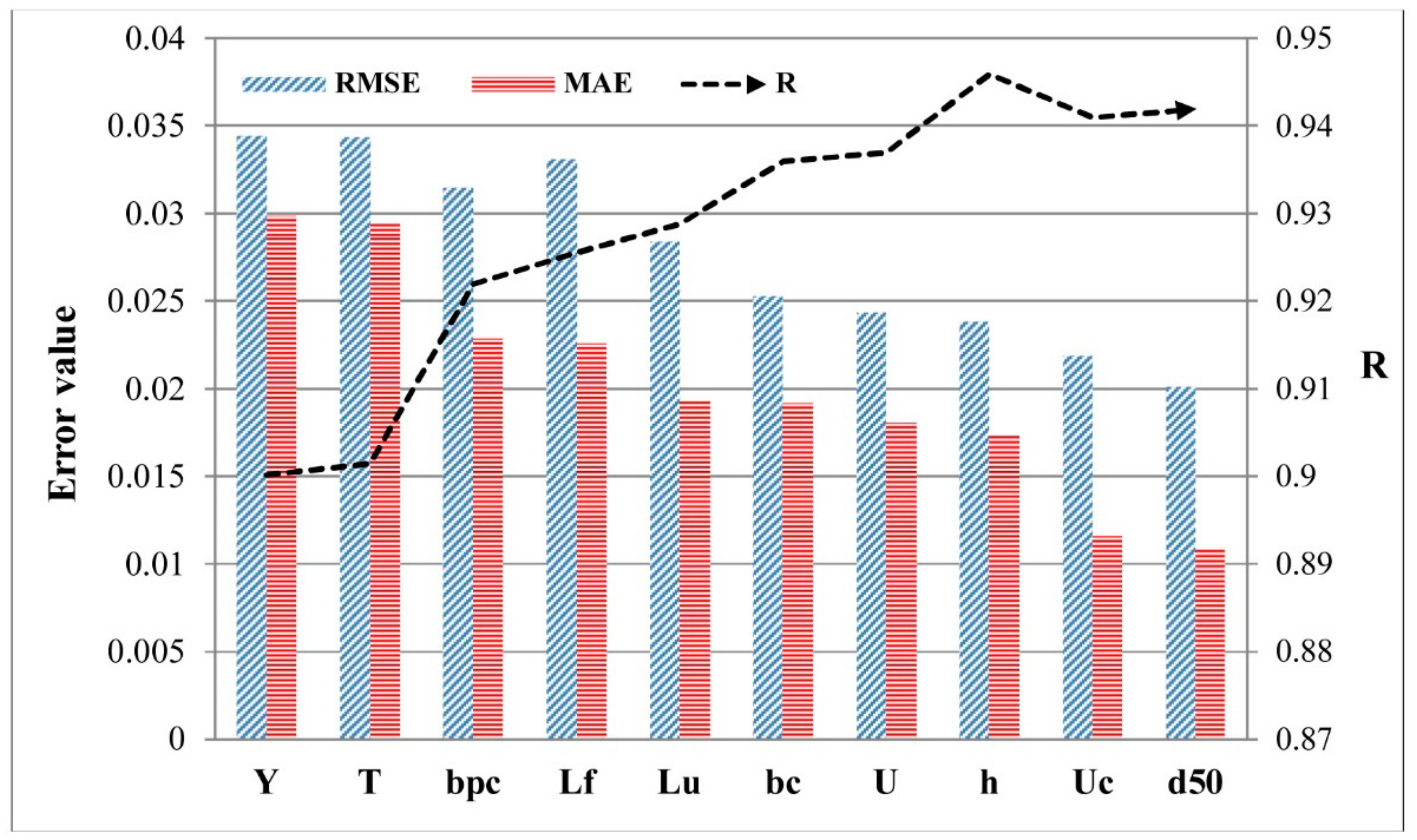
3.3. Sensitivity Analysis
4. Discussion
5. Conclusions
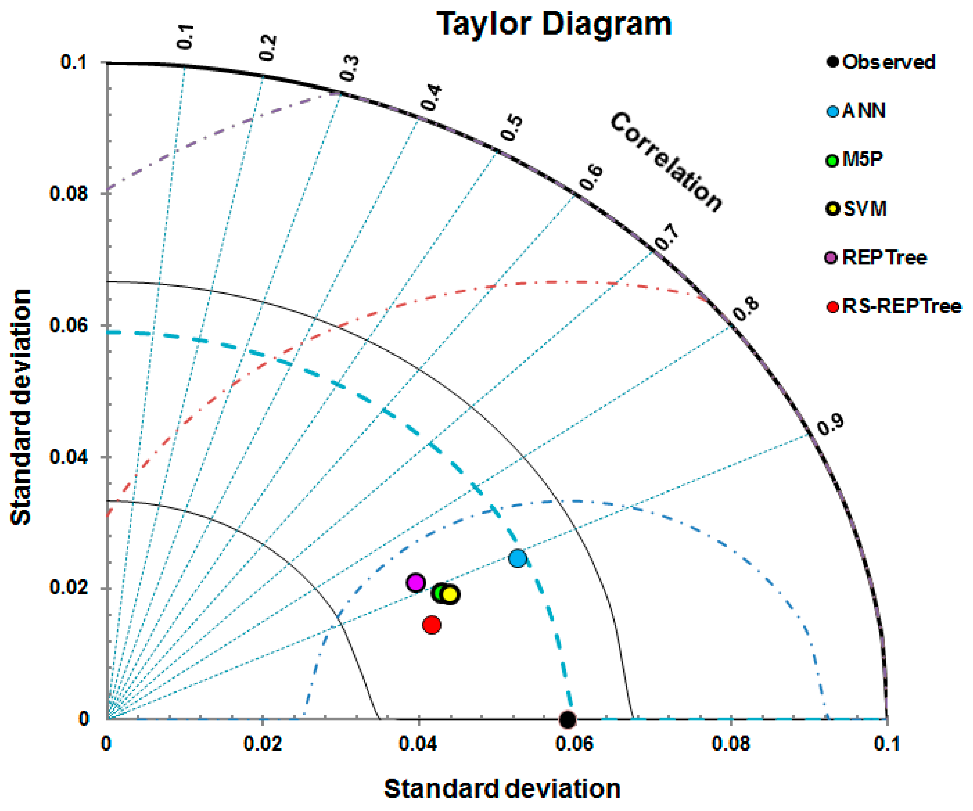
- The machine learning algorithms have the powerful capability to predict LSCP and the hybrid models can improve the performance of separate models in predicting LSCP.
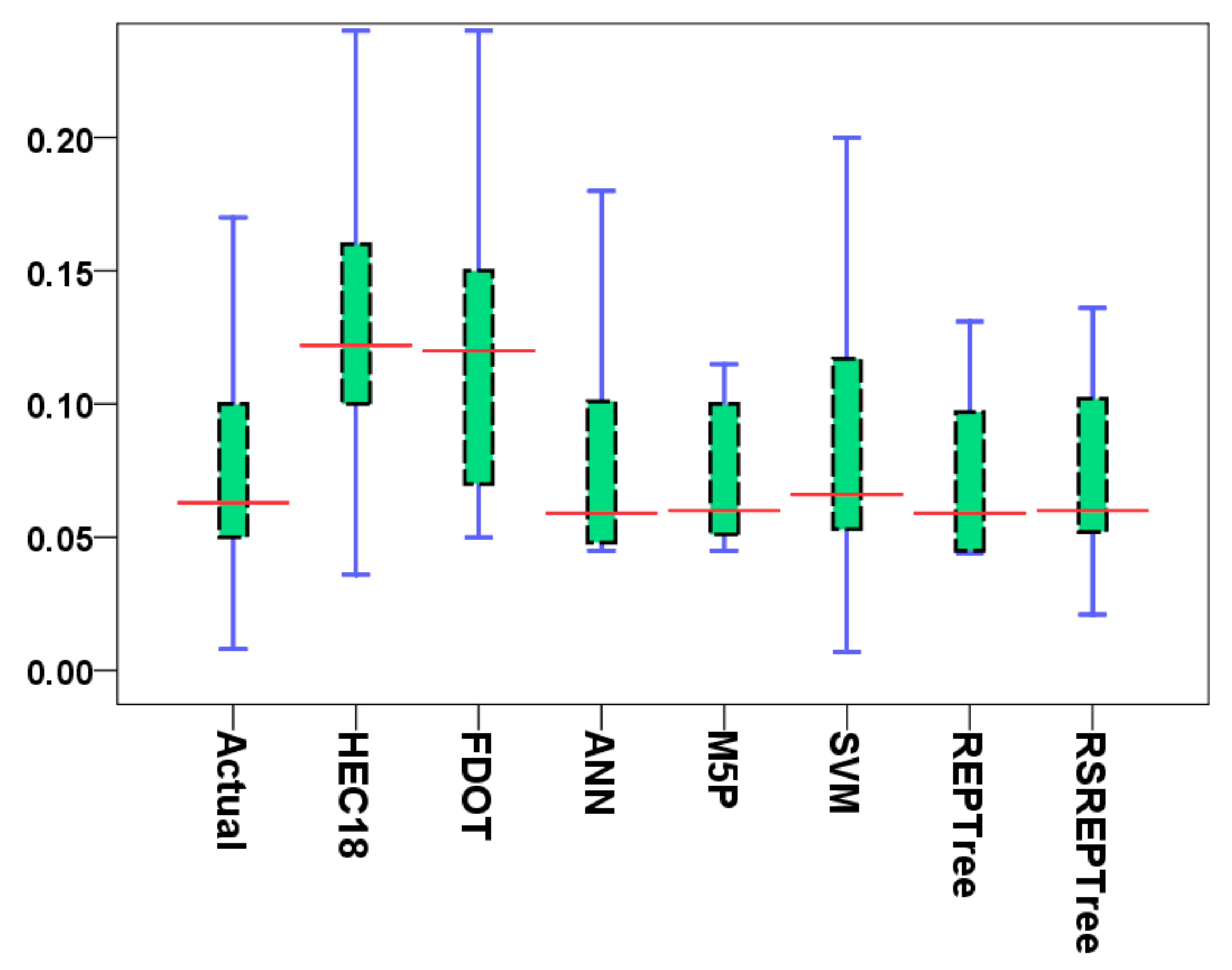
- Computing benchmark algorithms presented in this research have the potential to alter the LSCP prediction in comparison with the most well-known empirical methods, namely HEC-18 and FDOT methods.
- The state-of-the-art RS-REPTree ensemble model, with the highest accuracy of the REPTree, is proposed as a classifier for the prediction of the LSCP.
- The pile cap location (Y) was a more sensitive factor for LSCP among other factors based on the availability of data.
Author Contributions
Funding
Conflicts of Interest
Abbreviations
| RMSE | Root Mean Squared Error |
| LSCP | Local Scour Depth at Complex Piers |
| RS | Random Subspace |
| ANN | Artificial Neural Network |
| R | Correlation Coefficient |
| d50 | Median Sediment Size |
| Ys | Scour Depth |
| h | Water Depth |
| bc | Column Width |
| lc | Column Length |
| bpc | Pile Cap Width |
| lpc | Pile Cap Length |
| T | Pile Cap Thickness |
| Lu | Extension length of pile cap out from the column face |
| Lf | Extension width of pile cap out from the column |
| ksc | Shape factor for the column |
| kspc | Shape factor for the pile cap |
| bpg | Pile diameter |
| Fr | Froude number |
| m | Number of piles in line with the flow |
| n | Number of piles normal with the flow |
| Sl | Pile spacing in line with the flow |
| Sb | Pile spacing normal with the flow |
| Y | Pile cap elevation in respect to undisturbed streamflow |
| be | Equivalent width/diameter |
| yscol | Column’s scour |
| yspc | Pile cap’s scour |
| yspg | Scour of pile group |
| Dse | Equivalent diameters of the complex pier |
| Decol | Equivalent diameters of the column |
| Depc | Equivalent diameters of the pile cap |
| Depg | Equivalent diameters of the pile group |
| X | Training dataset |
| S | Subset of training dataset |
| Uc | Critical velocity for the beginning of sediment motion |
| U | Mean approach flow velocity |
References
- Lee, S.O.; Hong, S.H. Turbulence Characteristics before and after Scour Upstream of a Scaled-Down Bridge Pier Model. Water 2019, 11, 1900. [Google Scholar] [CrossRef]
- Melville, B.W.; Coleman, S.E. Bridge Scour; Water Resources Publication: Littleton, CO, USA, 2000. [Google Scholar]
- Ghodsi, H.; Khanjani, M.; Beheshti, A. Evaluation of harmony search optimization to predict local scour depth around complex bridge piers. Civ. Eng. J. 2018, 4, 402–412. [Google Scholar] [CrossRef]
- Ghazvinei, P.T.; Mohamed, T.A.; Ghazali, A.H.; Huat, B.K. Scour hazard assessment and bridge abutment instability analysis. Electron. J. Geotech. Eng. 2012, 17, 2213–2224. [Google Scholar]
- Wardhana, K.; Hadipriono, F.C. Analysis of recent bridge failures in the United States. J. Perform. Constr. Facil. 2003, 17, 144–150. [Google Scholar] [CrossRef]
- Amini, A.; Melville, B.W.; Ali, T.M. Local scour at piled bridge piers including an examination of the superposition method. Can. J. Civ. Eng. 2014, 41, 461–471. [Google Scholar] [CrossRef]
- Amini, A.; Mohammad, T.A. Local scour prediction around piers with complex geometry. Mar. Georesour. Geotechnol. 2017, 35, 857–864. [Google Scholar] [CrossRef]
- Baghbadorani, D.A.; Ataie-Ashtiani, B.; Beheshti, A.; Hadjzaman, M.; Jamali, M. Prediction of current-induced local scour around complex piers: Review, revisit, and integration. Coast. Eng. 2018, 133, 43–58. [Google Scholar] [CrossRef]
- Arneson, L.; Zevenbergen, L.; Lagasse, P.; Clopper, P. Evaluating Scour at Bridges; U.S. Department of TransportationFederal Highway Administration: Washington, DC, USA, 2012.
- Coleman, S.E. Clearwater local scour at complex piers. J. Hydraul. Eng. 2005, 131, 330–334. [Google Scholar] [CrossRef]
- Sheppard, D.; Renna, R. Bridge Scour Manual; Florida Department of Transportation: Tallahassee, FL, USA, 2005. [Google Scholar]
- Jannaty, M.; Eghbalzadeh, A.; Hosseini, S. Using field data to evaluate the complex bridge piers scour methods. Can. J. Civ. Eng. 2015, 43, 218–225. [Google Scholar] [CrossRef]
- Mueller, D.S.; Wagner, C.R. Field Observations and Evaluations of Streambed Scour at Bridges; U.S. Department of TransportationFederal Highway Administration: Washington, DC, USA, 2005.
- Chen, W.; Xie, X.; Wang, J.; Pradhan, B.; Hong, H.; Bui, D.T.; Duan, Z.; Ma, J. A comparative study of logistic model tree, random forest, and classification and regression tree models for spatial prediction of landslide susceptibility. Catena 2017, 151, 147–160. [Google Scholar] [CrossRef]
- Thai Pham, B.; Prakash, I.; Dou, J.; Singh, S.K.; Trinh, P.T.; Trung Tran, H.; Minh Le, T.; Tran, V.P.; Kim Khoi, D.; Shirzadi, A. A novel hybrid approach of landslide susceptibility modeling using rotation forest ensemble and different base classifiers. Geocarto Int. 2018, 14, 1–38. [Google Scholar]
- Shafizadeh-Moghadam, H.; Valavi, R.; Shahabi, H.; Chapi, K.; Shirzadi, A. Novel forecasting approaches using combination of machine learning and statistical models for flood susceptibility mapping. J. Environ. Manag. 2018, 217, 1–11. [Google Scholar] [CrossRef] [PubMed]
- Pham, B.T.; Prakash, I.; Singh, S.K.; Shirzadi, A.; Shahabi, H.; Bui, D.T. Landslide susceptibility modeling using Reduced Error Pruning Trees and different ensemble techniques: Hybrid machine learning approaches. Catena 2019, 175, 203–218. [Google Scholar] [CrossRef]
- Wang, Y.; Hong, H.; Chen, W.; Li, S.; Panahi, M.; Khosravi, K.; Shirzadi, A.; Shahabi, H.; Panahi, S.; Costache, R. Flood susceptibility mapping in dingnan county (China) using adaptive neuro-fuzzy inference system with biogeography based optimization and imperialistic competitive algorithm. J. Environ. Manag. 2019, 247, 712–729. [Google Scholar] [CrossRef] [PubMed]
- Ahmadlou, M.; Karimi, M.; Alizadeh, S.; Shirzadi, A.; Parvinnejhad, D.; Shahabi, H.; Panahi, M. Flood susceptibility assessment using integration of adaptive network-based fuzzy inference system (ANFIS) and biogeography-based optimization (BBO) and BAT algorithms (BA). Geocarto Int. 2019, 34, 1252–1272. [Google Scholar] [CrossRef]
- Khosravi, K.; Shahabi, H.; Pham, B.T.; Adamowski, J.; Shirzadi, A.; Pradhan, B.; Dou, J.; Ly, H.-B.; Gróf, G.; Ho, H.L. A comparative assessment of flood susceptibility modeling using Multi-Criteria Decision-Making Analysis and Machine Learning Methods. J. Hydrol. 2019, 573, 311–323. [Google Scholar] [CrossRef]
- Chen, W.; Hong, H.; Li, S.; Shahabi, H.; Wang, Y.; Wang, X.; Ahmad, B.B. Flood susceptibility modelling using novel hybrid approach of reduced-error pruning trees with bagging and random subspace ensembles. J. Hydrol. 2019, 575, 864–873. [Google Scholar] [CrossRef]
- Tien Bui, D.; Khosravi, K.; Shahabi, H.; Daggupati, P.; Adamowski, J.F.; M Melesse, A.; Thai Pham, B.; Pourghasemi, H.R.; Mahmoudi, M.; Bahrami, S. Flood spatial modeling in northern Iran using remote sensing and gis: A comparison between evidential belief functions and its ensemble with a multivariate logistic regression model. Remote Sens. 2019, 11, 1589. [Google Scholar] [CrossRef]
- Bui, D.T.; Panahi, M.; Shahabi, H.; Singh, V.P.; Shirzadi, A.; Chapi, K.; Khosravi, K.; Chen, W.; Panahi, S.; Li, S. Novel hybrid evolutionary algorithms for spatial prediction of floods. Sci. Rep. 2018, 8, 15364. [Google Scholar] [CrossRef]
- Tien Bui, D.; Khosravi, K.; Li, S.; Shahabi, H.; Panahi, M.; Singh, V.; Chapi, K.; Shirzadi, A.; Panahi, S.; Chen, W. New hybrids of anfis with several optimization algorithms for flood susceptibility modeling. Water 2018, 10, 1210. [Google Scholar] [CrossRef]
- Chen, W.; Pradhan, B.; Li, S.; Shahabi, H.; Rizeei, H.M.; Hou, E.; Wang, S. Novel hybrid integration approach of bagging-based fisher’s linear discriminant function for groundwater potential analysis. Nat. Resour. Res. 2019, 28, 1–20. [Google Scholar] [CrossRef]
- Miraki, S.; Zanganeh, S.H.; Chapi, K.; Singh, V.P.; Shirzadi, A.; Shahabi, H.; Pham, B.T. Mapping groundwater potential using a novel hybrid intelligence approach. Water Resour. Manag. 2019, 33, 281–302. [Google Scholar] [CrossRef]
- Rahmati, O.; Naghibi, S.A.; Shahabi, H.; Bui, D.T.; Pradhan, B.; Azareh, A.; Rafiei-Sardooi, E.; Samani, A.N.; Melesse, A.M. Groundwater spring potential modelling: Comprising the capability and robustness of three different modeling approaches. J. Hydrol. 2018, 565, 248–261. [Google Scholar] [CrossRef]
- Rahmati, O.; Choubin, B.; Fathabadi, A.; Coulon, F.; Soltani, E.; Shahabi, H.; Mollaefar, E.; Tiefenbacher, J.; Cipullo, S.; Ahmad, B.B. Predicting uncertainty of machine learning models for modelling nitrate pollution of groundwater using quantile regression and uneec methods. Sci. Total Environ. 2019, 688, 855–866. [Google Scholar] [CrossRef] [PubMed]
- Chen, W.; Li, Y.; Xue, W.; Shahabi, H.; Li, S.; Hong, H.; Wang, X.; Bian, H.; Zhang, S.; Pradhan, B. Modeling flood susceptibility using data-driven approaches of naïve Bayes tree, alternating decision tree, and random forest methods. Sci. Total Environ. 2020, 701, 134979. [Google Scholar] [CrossRef]
- Khosravi, K.; Melesse, A.M.; Shahabi, H.; Shirzadi, A.; Chapi, K.; Hong, H. Flood susceptibility mapping at Ningdu catchment, China using bivariate and data mining techniques. In Extreme Hydrology and Climate Variability; Elsevier: Amsterdam, The Netherlands, 2019; pp. 419–434. [Google Scholar]
- He, Q.; Shahabi, H.; Shirzadi, A.; Li, S.; Chen, W.; Wang, N.; Chai, H.; Bian, H.; Ma, J.; Chen, Y. Landslide spatial modelling using novel bivariate statistical based Naïve Bayes, RBF Classifier, and RBF Network machine learning algorithms. Sci. Total Environ. 2019, 663, 1–15. [Google Scholar] [CrossRef]
- Tien Bui, D.; Shirzadi, A.; Shahabi, H.; Chapi, K.; Omidavr, E.; Pham, B.T.; Talebpour Asl, D.; Khaledian, H.; Pradhan, B.; Panahi, M. A Novel Ensemble Artificial Intelligence Approach for Gully Erosion Mapping in a Semi-Arid Watershed (Iran). Sensors 2019, 19, 2444. [Google Scholar] [CrossRef]
- Tien Bui, D.; Shahabi, H.; Omidvar, E.; Shirzadi, A.; Geertsema, M.; Clague, J.J.; Khosravi, K.; Pradhan, B.; Pham, B.T.; Chapi, K. Shallow landslide prediction using a novel hybrid functional machine learning algorithm. Remote Sens. 2019, 11, 931. [Google Scholar] [CrossRef]
- Tien Bui, D.; Shirzadi, A.; Chapi, K.; Shahabi, H.; Pradhan, B.; Pham, B.T.; Singh, V.P.; Chen, W.; Khosravi, K.; Bin Ahmad, B. A Hybrid Computational Intelligence Approach to Groundwater Spring Potential Mapping. Water 2019, 11, 2013. [Google Scholar] [CrossRef]
- Tien Bui, D.; Shahabi, H.; Shirzadi, A.; Chapi, K.; Hoang, N.-D.; Pham, B.; Bui, Q.-T.; Tran, C.-T.; Panahi, M.; Bin Ahamd, B. A novel integrated approach of relevance vector machine optimized by imperialist competitive algorithm for spatial modeling of shallow landslides. Remote Sens. 2018, 10, 1538. [Google Scholar] [CrossRef]
- Chen, W.; Peng, J.; Hong, H.; Shahabi, H.; Pradhan, B.; Liu, J.; Zhu, A.-X.; Pei, X.; Duan, Z. Landslide susceptibility modelling using GIS-based machine learning techniques for Chongren County, Jiangxi Province, China. Sci. Total Environ. 2018, 626, 1121–1135. [Google Scholar] [CrossRef] [PubMed]
- Granata, F.; de Marinis, G. Machine learning methods for wastewater hydraulics. Flow Meas. Instrum. 2017, 57, 1–9. [Google Scholar] [CrossRef]
- Parasuraman, K.; Elshorbagy, A.; Si, B.C. Estimating saturated hydraulic conductivity in spatially variable fields using neural network ensembles. Soil Sci. Soc. Am. J. 2006, 70, 1851–1859. [Google Scholar] [CrossRef]
- Pham, B.T.; Hoang, T.-A.; Nguyen, D.-M.; Bui, D.T. Prediction of shear strength of soft soil using machine learning methods. Catena 2018, 166, 181–191. [Google Scholar] [CrossRef]
- Prasad, R.; Deo, R.C.; Li, Y.; Maraseni, T. Soil moisture forecasting by a hybrid machine learning technique: ELM integrated with ensemble empirical mode decomposition. Geoderma 2018, 330, 136–161. [Google Scholar] [CrossRef]
- Kazemi, S.; Minaei Bidgoli, B.; Shamshirband, S.; Karimi, S.M.; Ghorbani, M.A.; Chau, K.-W.; Kazem Pour, R. Novel genetic-based negative correlation learning for estimating soil temperature. Eng. Appl. Comput. Fluid Mech. 2018, 12, 506–516. [Google Scholar] [CrossRef]
- Chen, W.; Shahabi, H.; Shirzadi, A.; Hong, H.; Akgun, A.; Tian, Y.; Liu, J.; Zhu, A.-X.; Li, S. Novel hybrid artificial intelligence approach of bivariate statistical-methods-based kernel logistic regression classifier for landslide susceptibility modeling. Bull. Eng. Geol. Environ. 2019, 78, 4397–4419. [Google Scholar] [CrossRef]
- Jaafari, A.; Zenner, E.K.; Panahi, M.; Shahabi, H. Hybrid artificial intelligence models based on a neuro-fuzzy system and metaheuristic optimization algorithms for spatial prediction of wildfire probability. Agric. For. Meteorol. 2019, 266, 198–207. [Google Scholar] [CrossRef]
- Alizadeh, M.; Alizadeh, E.; Asadollahpour Kotenaee, S.; Shahabi, H.; Beiranvand Pour, A.; Panahi, M.; Bin Ahmad, B.; Saro, L. Social vulnerability assessment using artificial neural network (ANN) model for earthquake hazard in Tabriz city, Iran. Sustainability 2018, 10, 3376. [Google Scholar] [CrossRef]
- Chen, W.; Shirzadi, A.; Shahabi, H.; Ahmad, B.B.; Zhang, S.; Hong, H.; Zhang, N. A novel hybrid artificial intelligence approach based on the rotation forest ensemble and naïve Bayes tree classifiers for a landslide susceptibility assessment in Langao County, China. Geomat. Nat. Hazards Risk 2017, 8, 1955–1977. [Google Scholar] [CrossRef]
- Cheng, M.-Y.; Cao, M.-T. Hybrid intelligent inference model for enhancing prediction accuracy of scour depth around bridge piers. Struct. Infrastruct. Eng. 2015, 11, 1178–1189. [Google Scholar] [CrossRef]
- Najafzadeh, M.; Barani, G.-A.; Azamathulla, H.M. GMDH to predict scour depth around a pier in cohesive soils. Appl. Ocean. Res. 2013, 40, 35–41. [Google Scholar] [CrossRef]
- Zounemat-Kermani, M.; Beheshti, A.-A.; Ataie-Ashtiani, B.; Sabbagh-Yazdi, S.-R. Estimation of current-induced scour depth around pile groups using neural network and adaptive neuro-fuzzy inference system. Appl. Soft Comput. 2009, 9, 746–755. [Google Scholar] [CrossRef]
- Hosseini, R.; Fazloula, R.; Saneie, M.; Amini, A. Bagged neural network for estimating the scour depth around pile groups. Int. J. River Basin Manag. 2018, 16, 401–412. [Google Scholar] [CrossRef]
- Amini, A.; Ali, T.M.; Ghazali, A.H.; Aziz, A.A.; Akib, S.M. Impacts of land-use change on streamflows in the Damansara Watershed, Malaysia. Arab. J. Sci. Eng. 2011, 36, 713–720. [Google Scholar] [CrossRef]
- Amini, A.; Mohammad, T.A.; Aziz, A.A.; Ghazali, A.H.; Huat, B.B. A local scour prediction method for pile caps in complex piers. In Proceedings of the Institution of Civil Engineers-Water Management; ICE: Washington, DC, USA, 2019; pp. 73–80. [Google Scholar]
- Ataie-Ashtiani, B.; Baratian-Ghorghi, Z.; Beheshti, A. Experimental investigation of clear-water local scour of compound piers. J. Hydraul. Eng. 2010, 136, 343–351. [Google Scholar] [CrossRef]
- Rumelhart, D.E.; McClelland, J.L. Parallel Distributed Processing: Explorations in the Microstructure of Cognition, Volume 1. Foundations; MIT Press: Cambridge, MA, USA, 1986. [Google Scholar]
- Haykin, S. Support vector machines. Neural Netw. A Compr. Found. 1999, 12, 318–350. [Google Scholar]
- Dreiseitl, S.; Ohno-Machado, L. Logistic regression and artificial neural network classification models: A methodology review. J. Biomed. Inform. 2002, 35, 352–359. [Google Scholar] [CrossRef]
- Tian, Y.; Xu, C.; Hong, H.; Zhou, Q.; Wang, D. Mapping earthquake-triggered landslide susceptibility by use of artificial neural network (ANN) models: An example of the 2013 Minxian (China) Mw 5.9 event. Geomat. Nat. Hazards Risk 2019, 10, 1–25. [Google Scholar] [CrossRef]
- Shirzadi, A.; Shahabi, H.; Chapi, K.; Bui, D.T.; Pham, B.T.; Shahedi, K.; Ahmad, B.B. A comparative study between popular statistical and machine learning methods for simulating volume of landslides. Catena 2017, 157, 213–226. [Google Scholar] [CrossRef]
- Bateni, S.M.; Borghei, S.; Jeng, D.-S. Neural network and neuro-fuzzy assessments for scour depth around bridge piers. Eng. Appl. Artif. Intell. 2007, 20, 401–414. [Google Scholar] [CrossRef]
- Kia, M.B.; Pirasteh, S.; Pradhan, B.; Mahmud, A.R.; Sulaiman, W.N.A.; Moradi, A. An artificial neural network model for flood simulation using GIS: Johor River Basin, Malaysia. Environ. Earth Sci. 2012, 67, 251–264. [Google Scholar] [CrossRef]
- Kaya, A. Artificial neural network study of observed pattern of scour depth around bridge piers. Comput. Geotech. 2010, 37, 413–418. [Google Scholar] [CrossRef]
- Choi, S.U.; Cheong, S. Prediction of local scour around bridge piers using artificial neural networks 1. J. Am. Water Resour. Assoc. 2006, 42, 487–494. [Google Scholar] [CrossRef]
- Pal, M.; Singh, N.; Tiwari, N. Support vector regression based modeling of pier scour using field data. Eng. Appl. Artif. Intell. 2011, 24, 911–916. [Google Scholar] [CrossRef]
- Quinlan, J.R. Learning with continuous classes. In Proceedings of the 5th Australian Joint Conference on Artificial Intelligence, Hobart, Tasmania, 16–18 November 1992; pp. 343–348. [Google Scholar]
- Balouchi, B.; Nikoo, M.R.; Adamowski, J. Development of expert systems for the prediction of scour depth under live-bed conditions at river confluences: Application of different types of ANNs and the M5P model tree. Appl. Soft Comput. 2015, 34, 51–59. [Google Scholar] [CrossRef]
- Etemad-Shahidi, A.; Mahjoobi, J. Comparison between M5′ model tree and neural networks for prediction of significant wave height in Lake Superior. Ocean Eng. 2009, 36, 1175–1181. [Google Scholar] [CrossRef]
- Solomatine, D.P.; Siek, M.B.L. Flexible and optimal M5 model trees with applications to flow predictions. In Hydroinformatics: (In 2 Volumes, with CD-ROM); World Scientific: Singapore, 2004; pp. 1719–1726. [Google Scholar]
- Bhattacharya, B.; Solomatine, D.P. Neural networks and M5 model trees in modelling water level–discharge relationship. Neurocomputing 2005, 63, 381–396. [Google Scholar] [CrossRef]
- Vapnik, V. The Nature of Statistical Learning Theory; Jordan, M., Lauritzen, S.L., Lawless, J.L., Nair, V., Eds.; Springer: NewYork, NY, USA, 1995. [Google Scholar]
- Micheletti, N.; Foresti, L.; Robert, S.; Leuenberger, M.; Pedrazzini, A.; Jaboyedoff, M.; Kanevski, M. Machine learning feature selection methods for landslide susceptibility mapping. Math. Geosci. 2014, 46, 33–57. [Google Scholar] [CrossRef]
- Vapnik, V. Pattern recognition using generalized portrait method. Autom. Remote Control 1963, 24, 774–780. [Google Scholar]
- Quinlan, J.R. Simplifying decision trees. Int. J. Man-Mach. Stud. 1987, 27, 221–234. [Google Scholar] [CrossRef]
- Khosravi, K.; Pham, B.T.; Chapi, K.; Shirzadi, A.; Shahabi, H.; Revhaug, I.; Prakash, I.; Bui, D.T. A comparative assessment of decision trees algorithms for flash flood susceptibility modeling at Haraz watershed, northern Iran. Sci. Total Environ. 2018, 627, 744–755. [Google Scholar] [CrossRef]
- Mohamed, W.N.H.W.; Salleh, M.N.M.; Omar, A.H. A comparative study of reduced error pruning method in decision tree algorithms. In Proceedings of the Control System, Computing and Engineering (ICCSCE), 2012 IEEE International Conference on, Penang, Malaysian, 23 November 2012; pp. 392–397. [Google Scholar]
- Galathiya, A.; Ganatra, A.; Bhensdadia, C. Improved decision tree induction algorithm with feature selection, cross validation, model complexity and reduced error pruning. Int. J. Comput. Sci. Inf. Technol. 2012, 3, 3427–3431. [Google Scholar]
- Ho, T.K. The random subspace method for constructing decision forests. IEEE Trans. Pattern Anal. Mach. Intell. 1998, 20, 832–844. [Google Scholar]
- Skurichina, M.; Duin, R.P. Bagging, boosting and the random subspace method for linear classifiers. Pattern Anal. Appl. 2002, 5, 121–135. [Google Scholar] [CrossRef]
- Shirzadi, A.; Bui, D.T.; Pham, B.T.; Solaimani, K.; Chapi, K.; Kavian, A.; Shahabi, H.; Revhaug, I. Shallow landslide susceptibility assessment using a novel hybrid intelligence approach. Environ. Earth Sci. 2017, 76, 60. [Google Scholar] [CrossRef]
- Chai, T.; Draxler, R.R. Root mean square error (RMSE) or mean absolute error (MAE)?–Arguments against avoiding RMSE in the literature. Geosci. Model. Dev. 2014, 7, 1247–1250. [Google Scholar] [CrossRef]
- Willmott, C.J.; Matsuura, K. Advantages of the mean absolute error (MAE) over the root mean square error (RMSE) in assessing average model performance. Clim. Res. 2005, 30, 79–82. [Google Scholar] [CrossRef]
- Veerasamy, R.; Rajak, H.; Jain, A.; Sivadasan, S.; Varghese, C.P.; Agrawal, R.K. Validation of QSAR models-strategies and importance. Int. J. Drug Des. Discov. 2011, 3, 511–519. [Google Scholar]
- Bonadonna, C.; Costa, A. Estimating the volume of tephra deposits: A new simple strategy. Geology 2012, 40, 415–418. [Google Scholar] [CrossRef]
- Taylor, K.E. Summarizing multiple aspects of model performance in a single diagram. J. Geophys. Res. Atmos. 2001, 106, 7183–7192. [Google Scholar] [CrossRef]
- Sigaroodi, S.K.; Chen, Q.; Ebrahimi, S.; Nazari, A.; Choobin, B. Long-term precipitation forecast for drought relief using atmospheric circulation factors: A study on the Maharloo Basin in Iran. Hydrol. Earth Syst. Sci. 2014, 18, 1995–2006. [Google Scholar] [CrossRef]
- Barnston, A.G. Correspondence among the correlation, RMSE, and Heidke forecast verification measures; refinement of the Heidke score. Weather Forecast. 1992, 7, 699–709. [Google Scholar] [CrossRef]
- Chapi, K.; Singh, V.P.; Shirzadi, A.; Shahabi, H.; Bui, D.T.; Pham, B.T.; Khosravi, K. A novel hybrid artificial intelligence approach for flood susceptibility assessment. Environ. Model. Softw. 2017, 95, 229–245. [Google Scholar] [CrossRef]
- Najafzadeh, M.; Rezaie Balf, M.; Rashedi, E. Prediction of maximum scour depth around piers with debris accumulation using EPR, MT, and GEP models. J. Hydroinform. 2016, 18, 867–884. [Google Scholar] [CrossRef]
- Beasley, T.M.; Zumbo, B.D. Comparison of aligned Friedman rank and parametric methods for testing interactions in split-plot designs. Comput. Stat. Data Anal. 2003, 42, 569–593. [Google Scholar] [CrossRef]
- Lee, S.O.; Hong, S.H. Reproducing Field Measurements Using Scaled-Down Hydraulic Model Studies in a Laboratory. Adv. Civ. Eng. 2018, 2018, 1–11. [Google Scholar] [CrossRef]
- Moreno, M.; Maia, R.; Couto, L. Effects of relative column width and pile-cap elevation on local scour depth around complex piers. J. Hydraul. Eng. 2015, 142, 04015051. [Google Scholar] [CrossRef]
- Ferraro, D.; Tafarojnoruz, A.; Gaudio, R.; Cardoso, A.H. Effects of pile cap thickness on the maximum scour depth at a complex pier. J. Hydraul. Eng. 2013, 139, 482–491. [Google Scholar] [CrossRef]
- Amini, A.; Solaimani, N. The effects of uniform and nonuniform pile spacing variations on local scour at pile groups. Mar. Georesour. Geotechnol. 2018, 36, 861–866. [Google Scholar] [CrossRef]
- Shirzadi, A.; Soliamani, K.; Habibnejhad, M.; Kavian, A.; Chapi, K.; Shahabi, H.; Chen, W.; Khosravi, K.; Thai Pham, B.; Pradhan, B. Novel GIS based machine learning algorithms for shallow landslide susceptibility mapping. Sensors 2018, 18, 3777. [Google Scholar] [CrossRef] [PubMed]
- Shirzadi, A.; Solaimani, K.; Roshan, M.H.; Kavian, A.; Chapi, K.; Shahabi, H.; Keesstra, S.; Ahmad, B.B.; Bui, D.T. Uncertainties of prediction accuracy in shallow landslide modeling: Sample size and raster resolution. Catena 2019, 178, 172–188. [Google Scholar] [CrossRef]


| Algorithms | Parameters |
|---|---|
| ANN | Number of hidden layer: 7; learning rate: 0.3; momentue: 0.2; Number of seed: 3; training time: 500; validation threshold: 20; validation set size: default |
| M5P | Build regression tree: True; minimum number of instance: 4 |
| SVM | C: 0.95; filter type: normalized training data; regOptimizer: RegSMO improved; number of seed: 1; tolerance: 0.001 |
| REPTree | Maximum depth: −1; minimum number: 2; minimum variance probability: 0.001; number of fold: 2; number of seed: 1 |
| RS-REPTree | Classifier: REPTree; Number of iteration: 10; number of seed: 6; subspace size: 0.5 |
| Models | MAE | RMSE | R | |||
|---|---|---|---|---|---|---|
| Training | Validation | Training | Validation | Training | Validation | |
| FDOT | 0.045 | 0.058 | 0.032 | 0.062 | 0.736 | 0.726 |
| HEC-18 | 0.053 | 0.051 | 0.067 | 0.064 | 0.625 | 0.620 |
| ANN | 0.012 | 0.016 | 0.015 | 0.021 | 0.954 | 0.907 |
| M5P | 0.014 | 0.017 | 0.020 | 0.022 | 0.943 | 0.912 |
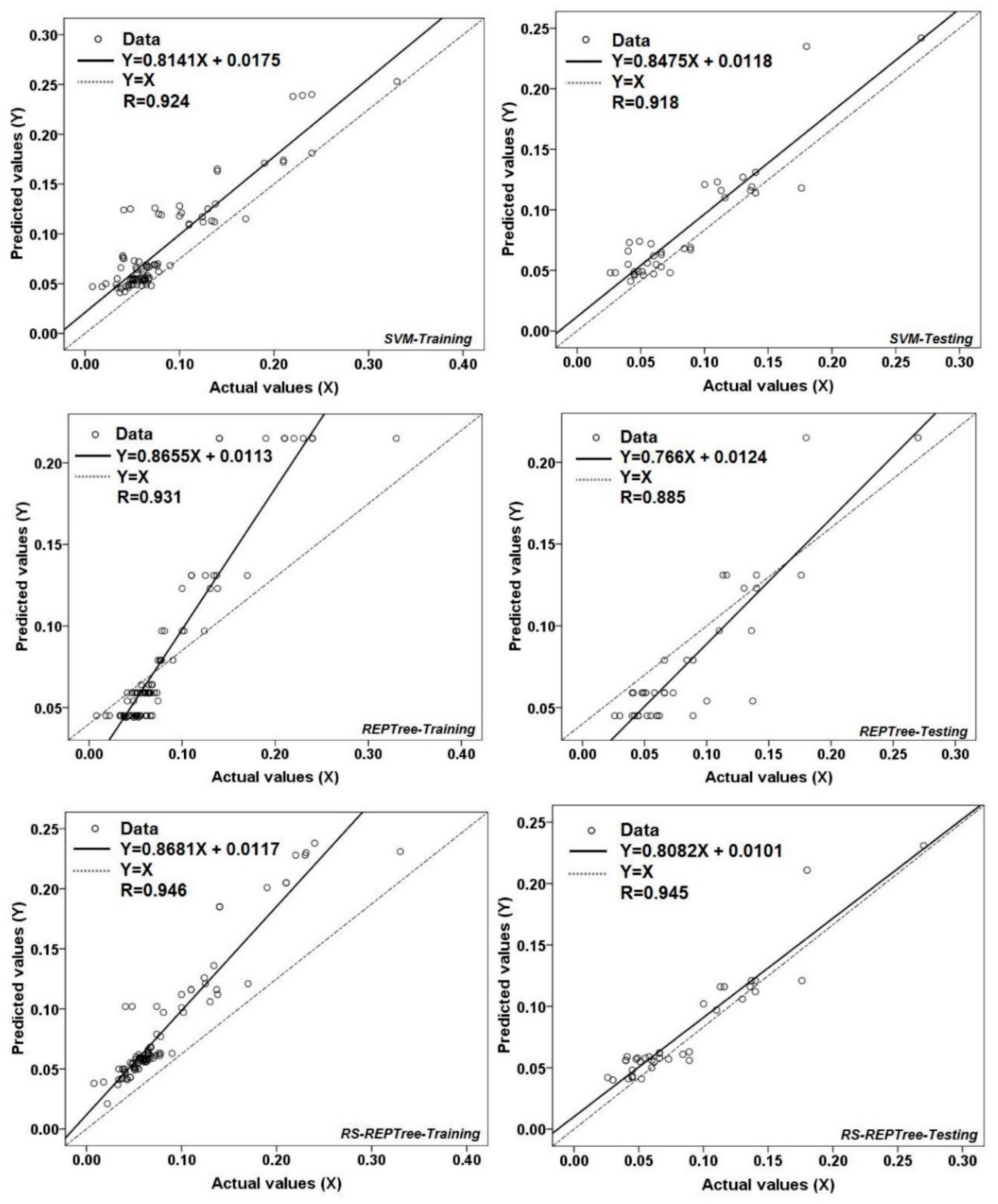
| SVM | 0.015 | 0.016 | 0.020 | 0.024 | 0.924 | 0.918 |
| REPTree | 0.013 | 0.018 | 0.021 | 0.025 | 0.931 | 0.885 |
| RS-REPTree | 0.013 | 0.014 | 0.019 | 0.018 | 0.946 | 0.945 |
| No | Scour Depth Models | Mean Ranks | χ2 | Sig. |
|---|---|---|---|---|
| 1 | FDOT | 6.53 | 158.012 | 0.000 |
| 2 | HEC-18 | 6.49 | ||
| 3 | ANN | 3.77 | ||
| 4 | M5P | 3.62 | ||
| 5 | SVM | 4.18 | ||
| 6 | REPTree | 3.58 | ||
| 7 | RS-REPTree | 3.38 |
| NO | Pairwise Comparison | NND | NPD | z-Value | p-Value | Significance |
|---|---|---|---|---|---|---|
| 1 | Actual-FDOT | 9 | 65 | −6.608 | 0.000 | Yes |
| 2 | Actual-HEC18 | 14 | 68 | −6.732 | 0.000 | Yes |
| 3 | Actual-ANN | 39 | 44 | −0.409 | 0.683 | No |
| 4 | Actual-M5P | 45 | 39 | −0.085 | 0.932 | No |
| 5 | Actual-SVM | 37 | 38 | −0.481 | 0.631 | No |
| 6 | Actual-REPTree | 45 | 39 | −0.112 | 0.911 | No |
| 7 | Actual-RSREPTree | 41 | 40 | −0.443 | 0.658 | No |
| 8 | HEC18-FDOT | 40 | 24 | −0.994 | 0.320 | No |
| 9 | HEC18-ANN | 68 | 14 | −6.619 | 0.000 | Yes |
| 10 | HEC18-M5P | 74 | 10 | −6.927 | 0.000 | Yes |
| 11 | HEC18-SVM | 68 | 16 | −6.442 | 0.000 | Yes |
| 12 | HEC18-REPTree | 70 | 15 | −6.806 | 0.000 | Yes |
| 13 | HEC18-RSREPTree | 71 | 13 | −6.848 | 0.000 | Yes |
| 14 | FDOT-ANN | 78 | 10 | −6.799 | 0.000 | Yes |
| 15 | FDOT-M5P | 73 | 12 | −6.768 | 0.000 | Yes |
| 16 | FDOT-SVM | 67 | 18 | −6.536 | 0.000 | Yes |
| 17 | FDOT-REPTree | 78 | 7 | −7.072 | 0.000 | Yes |
| 18 | FDOT-RSREPTree | 67 | 13 | −6.799 | 0.000 | Yes |
| 19 | ANN-M5P | 40 | 39 | −0.364 | 0.716 | No |
| 20 | ANN-SVM | 32 | 50 | −1.371 | 0.170 | No |
| 21 | ANN-REPTree | 49 | 32 | −0.393 | 0.694 | No |
| 22 | ANN-RSREPTree | 37 | 47 | −0.116 | 0.908 | No |
| 23 | M5P-SVM | 36 | 46 | −1.318 | 0.188 | No |
| 24 | M5P-REPTree | 42 | 36 | −0.416 | 0.677 | No |
| 25 | M5P-RSREPTree | 35 | 49 | −0.989 | 0.323 | No |
| 26 | SVM-REPTree | 46 | 39 | −0.734 | 0.463 | No |
| 27 | SVM-RSREPTree | 47 | 36 | −01.115 | 0.265 | No |
| 28 | RSREPTree-RSREPTree | 43 | 37 | −0.187 | 0.852 | No |
© 2020 by the authors. Licensee MDPI, Basel, Switzerland. This article is an open access article distributed under the terms and conditions of the Creative Commons Attribution (CC BY) license (http://creativecommons.org/licenses/by/4.0/).
Share and Cite
Tien Bui, D.; Shirzadi, A.; Amini, A.; Shahabi, H.; Al-Ansari, N.; Hamidi, S.; Singh, S.K.; Thai Pham, B.; Ahmad, B.B.; Ghazvinei, P.T. A Hybrid Intelligence Approach to Enhance the Prediction Accuracy of Local Scour Depth at Complex Bridge Piers. Sustainability 2020, 12, 1063. https://doi.org/10.3390/su12031063
Tien Bui D, Shirzadi A, Amini A, Shahabi H, Al-Ansari N, Hamidi S, Singh SK, Thai Pham B, Ahmad BB, Ghazvinei PT. A Hybrid Intelligence Approach to Enhance the Prediction Accuracy of Local Scour Depth at Complex Bridge Piers. Sustainability. 2020; 12(3):1063. https://doi.org/10.3390/su12031063
Chicago/Turabian StyleTien Bui, Dieu, Ataollah Shirzadi, Ata Amini, Himan Shahabi, Nadhir Al-Ansari, Shahriar Hamidi, Sushant K. Singh, Binh Thai Pham, Baharin Bin Ahmad, and Pezhman Taherei Ghazvinei. 2020. "A Hybrid Intelligence Approach to Enhance the Prediction Accuracy of Local Scour Depth at Complex Bridge Piers" Sustainability 12, no. 3: 1063. https://doi.org/10.3390/su12031063
APA StyleTien Bui, D., Shirzadi, A., Amini, A., Shahabi, H., Al-Ansari, N., Hamidi, S., Singh, S. K., Thai Pham, B., Ahmad, B. B., & Ghazvinei, P. T. (2020). A Hybrid Intelligence Approach to Enhance the Prediction Accuracy of Local Scour Depth at Complex Bridge Piers. Sustainability, 12(3), 1063. https://doi.org/10.3390/su12031063