Analysis of the Insertion Angle of Lane-Changing Vehicles in Nearly Saturated Fast Road Segments

Abstract

Vehicle lane changing in a nearly saturated fast road segment tends to increase the probability of traffic accidents in the road segment and reduce the speed of the rear vehicles in the target lane. To better analyze the relationship between the target vehicle and the front and rear vehicles in the target lane, this study focuses on the insertion angle of the target vehicle as the research object. Moreover, this study considers influencing factors, such as the longitudinal distance, transverse distance, and speed of the front and rear vehicles in the target lane. This study also adopts aerial photography to capture the flow of the main road of the Xi’an South Second Ring Road, Chang’an University segment. Information regarding the vehicle captured on video, including the speed, insertion angle, and coordinates, is extracted using the software Tracker. The coordinates correlation and speed correlation are analyzed using the software SPSS 2.0. K-means cluster analysis is applied to cluster the insertion angle of the target vehicle, and the insertion speed of the target vehicle. Of the total samples, 89.47% were inserted into the target lane at around 23° or below. The PC-Crash software was used to verify that the collision consequences gradually increased with the increase in collision angle. Therefore, when the insertion angle of the vehicle changes to lower than 23°, the overall road traffic condition is optimal, and no large losses are incurred.

1. Introduction

Lane changing is one of the most common vehicle driving behaviors in fast road segments. Lane changing can improve the running speed of the target vehicle to a certain extent; however, Sun and Ondyli [1] found that a vehicle lane change can affect the running speed of the target lane and the lane vehicle in saturated traffic state. Zheng et al. [2] also indicated that vehicle lane change is a principal cause of traffic accidents, such as rear-end collision, side collision, and other accidents. A study on vehicle lane change conducted by Shuan et al. [3] showed that traffic accidents caused by direct or indirect lane changes comprised 15.8% of total traffic accidents. Lee et al. [4] indicated that collision accidents caused by vehicle lane changes comprised 4%–10% of total accidents. To reduce vehicle lane change accidents, several analyses have been conducted: Stephens and Groeger [5] examined the emotional characteristics of drivers, Hicks and Gilbert [6] explored the personality characteristics of drivers, Tian et al. [7] investigated road conditions, and National Highway Traffic Safety Administration [8] evaluated vehicle conditions. The most widely used lane change models are the regular lane change model proposed by Gipps [9] and the random utility lane change model proposed by Ahmed et al. [10]. Kesting et al. [11] proposed the total braking model caused by a minimum lane change, deduced vehicle lane change rules, and concluded that acceleration determines the risk associated with lane change. Ahmed [12] studied lane change decisions, target lane selection, and insertion gap in the decision process based on the random utility lane change model, and constructed a dynamic discrete selection model. Deng and Feng [13] designed a multi-lane cellular automatic machine lane change model by analyzing the internal and external factors affecting lane change, and concluded that lane-changing behavior can affect the running speed of the surrounding vehicles. Lee et al. [14] evaluated the effects of speed and spacing by using Next-Generation Simulation or NGSIM data to develop an exponential probability model of the differences in speed and lead gap between the target lane and the original lane. Bhadeshia [15] estimated that the angle applied to a high-speed vehicle for lane change is generally 5°. The aforementioned studies analyzed the influencing factors affecting lane change, as well as the change in the lane change model and change in angle for lane change angle under high-speed driving.

Two types of traffic flow definition in the fast road segment are identified: One is the unsaturated state that occurs when road traffic volume is less than road capacity, as opposed to the unsaturated state that occurs when the ratio of traffic volume to traffic capacity is less than 1. The traffic load classification standard refers to the US ‘’Highway Capacity Manual 2010” [16]. The other type is the supersaturated state first defined by Gazis et al. [17,18] as the condition when the ratio of traffic volume to saturation flow is greater than 1, minus the ratio of lost time to the signal cycle. Green [19] defines the supersaturated state as the condition when the ratio of traffic to saturated flow is greater than 1. In the nearly saturated state, the load of a vehicle in a fast-road segment of a city is relatively high compared with the peak–peak period, and the traffic load degree of the segment is constantly changing in the form of unsaturated to saturated to unsaturated state. In the current study, the nearly saturated state is said to occur when traffic flow is between 0.85 and 1. Traffic flow in the nearly saturated state is mainly indicated by an unstable traffic flow, traffic congestion, and drivers being unable to withstand the situation.

Most studies have focused on lane changing in a free-flow state road segment or intersection, but few have reported on the angle of insertion of the lane-changing vehicle under high-traffic density conditions. Therefore, it is important to analyze the angle of insertion of the lane-changing vehicle into the target lane when the traffic load of the fast road segment is in the 0.85–0.95 range.

2. Materials and Methods

2.1. Data Collection

Road conditions: The fast road should be separate from auxiliary roads, have a good view, and be free from interference from pedestrians and bicycles.

Data extraction: A DJI Phantom 4 drone was used to photograph the road vertically. The Tracker software was used to track the target vehicle, as well as the front and rear vehicles, in the target lane. The software tracked the data according to 1/30 s. Tracker software can provide an automatic and realistic analysis and processing scene [20].

The fast road of the South Second Ring Road of Xi’an was selected as the location of traffic video collection. The headquarters of Chang’an University was chosen as the video recording point. The fast road in the road segment was separate from the vehicles entering and leaving the fast road through the guardrail, and the vehicle lane change caused by vehicle entry or exit was eliminated. The single-lane width wad 3.75 m. Figure 4 is the road simulation diagram. The video was randomly shot from 200 m during the evening peak (17:00–18:00) on a weekday (12 August 2019). Shooting was conducted on a holiday in August, when most students were on vacation; regardless, the holiday only slightly affected the numbers of people driving because only a small proportion of students drove to school when they are not on holiday. The late peak period was the same as that considered in the study by Lijie et al. [21]. A total of 5607 pieces of data for 18 vehicles were extracted using the Tracker software. Figure 1 shows the video shooting area. Table 1 lists 20 sample data, which can provide data support for thesis analysis.

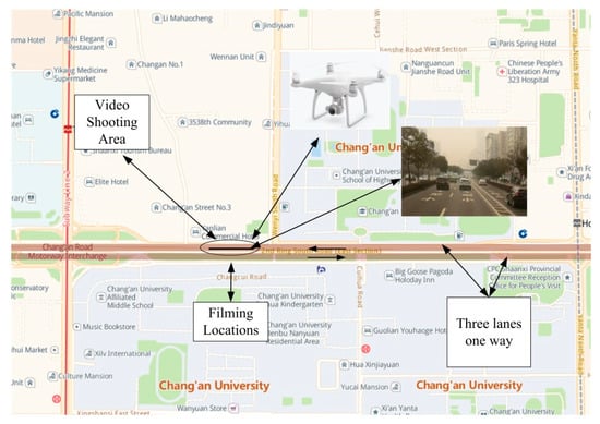
Figure 1. Location of video shooting.

Table 1. Some sample data.

No.	TVXC	TVYC	TVIS	TLFVXC	TLFVYC	TLFVS	TLRVXC	TLRVYC	TLRVS	TVIA
1	7.028	4.941	1.774	12.091	2.300	5.024	4.253	2.058	2.881	29.78
2	7.055	4.916	0.984	12.226	2.305	4.387	4.194	2.055	1.630	30.28
3	7.087	4.911	1.471	12.383	2.310	4.751	4.145	2.057	1.849	30.45
4	7.153	4.907	1.538	12.543	2.302	4.509	4.070	2.059	1.723	30.50
5	7.189	4.899	1.701	12.684	2.311	4.362	4.030	2.060	1.810	31.57
6	7.262	4.874	1.477	12.833	2.313	4.881	3.949	2.061	1.727	31.35
7	7.275	4.851	1.547	13.010	2.312	4.589	3.914	2.061	1.959	29.04
8	7.355	4.831	1.890	13.140	2.315	3.915	3.819	2.061	2.502	29.79
9	7.392	4.804	1.823	13.271	2.310	4.917	3.747	2.060	2.133	29.07
10	7.470	4.789	1.844	13.468	2.309	4.904	3.676	2.060	2.350	28.95
11	7.511	4.773	1.812	13.598	2.313	4.640	3.591	2.063	1.895	28.71
12	7.586	4.755	1.929	13.777	2.310	5.058	3.550	2.060	1.897	28.91
13	7.625	4.713	2.279	13.936	2.315	4.613	3.464	2.064	2.602	27.65
14	7.729	4.705	2.270	14.085	2.319	4.879	3.376	2.065	2.244	27.65
15	7.770	4.670	1.774	14.261	2.322	4.889	3.314	2.061	1.970	26.59
16	7.840	4.664	1.707	14.411	2.318	4.236	3.245	2.066	2.598	27.08
17	7.869	4.613	2.080	14.544	2.323	4.829	3.141	2.066	2.676	24.88
18	7.962	4.597	3.006	14.734	2.322	4.789	3.066	2.066	2.357	25.12
19	8.068	4.588	2.234	14.864	2.319	4.831	2.984	2.065	2.549	25.19
20	8.092	4.525	2.317	15.056	2.318	5.041	2.896	2.069	2.764	21.52

Notes: TVXC, Target Vehicle X-Coordinate; TVYS, Target Vehicle Y-Coordinate; TVIS, Target Vehicle Insertion Speed (m/s); TLFVXC, Target Lane Front Vehicle X-Coordinate; TLFVYC, Target Lane Front Vehicle Y-Coordinate; TLFVS, Target Lane Front Vehicle Speed (m/s); TLRVXC, Target Lane Rear Vehicle X-Coordinate; TLRVYC, Target Lane Rear Vehicle Y-Coordinate; TLRVS, Target Lane Rear Vehicle Speed (m/s); TVIA, Target Vehicle Insertion Angle (°).

2.2. Data Analysis Method

In order to obtain accurate data and determine the correct data analysis methods, a flowchart, including data survey, data extraction, and data analysis, was developed. Figure 2 reflects the series of processes from data acquisition to simulation feedback.

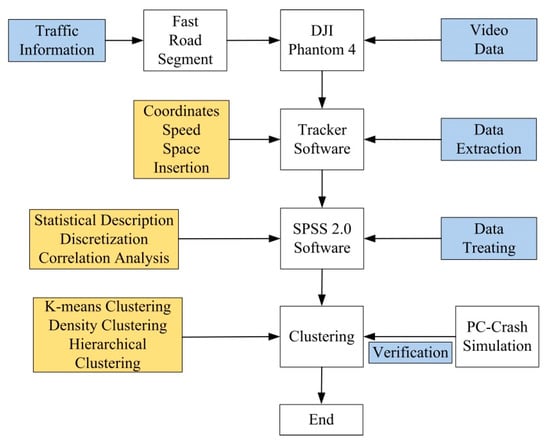
Figure 2. Data extraction and analysis.

2.2.1. Statistical Method

SPSS 2.0 was used to analyze the data extracted using the Tracker software, mainly analyzing the correlation between various influencing factors. The target vehicle insertion angle, speed, and distance between the front and rear vehicles in the target lane were investigated. The SPSS 2.0 software provides complete data analysis, including data acquisition, data processing, data analysis, and result presentation.

2.2.2. Clustering Method

Clustering is one of the most widely used techniques for exploratory data analysis. In this study, the insertion angle, speed, and spacing of vehicles with similar behaviors are determined based on the angle of insertion of the target vehicle into the target lane, the speed, as well the front- and rear-lane spacing of the target lane. The differentiation of objects and understanding the similarity between them [22], as well as aggregation of similar data, are essential components of data analysis, together with extracting similar data sets in unordered data. Common clustering methods include K-means clustering, density clustering, and system clustering [21].

(1) K-means Clustering

K-means is a clustering algorithm based on the partitioning ideas proposed by Macqueen [23]. The method entails clustering samples with a high degree of similarity into one class and those with, and the similarity between different clusters varies to a certain extent. Multiple data are divided into clusters of similar objects, with the sum of the squares of the data to the central data in each cluster being the smallest. The main steps of the method are as follows: Dividing the data into c clusters k₁, k₂, k₃……k_c and selecting one central point p₁, p₂, p₃……p_c from each cluster. n_j is the number of cluster k_j.

$$J={\displaystyle \sum _{i=1}^k{\displaystyle \sum _{j=1}^{{{\displaystyle n}}_j}{{\displaystyle d}}_{ij}\left({{\displaystyle x}}_j,{{\displaystyle p}}_i\right)}},{{\displaystyle p}}_i=\frac{1}{{{\displaystyle n}}_j}{\displaystyle \sum _{{{\displaystyle x}}_j\in {{\displaystyle k}}_j}{{\displaystyle x}}_j}$$

(1)

where d_ij(x_j, p_i) is the Euclidean distance between x_j and p_i cluster k_i.

(2) Density Clustering

Density-based clustering is premised on the density of the spatial distribution of the data. This clustering technique does not need to set clustering clusters in advance, and the data points in a given cluster contain at least several data points in a regional station within a certain distance from the point. Clustering can cluster high-density areas and locate clusters with arbitrary shapes in the space with noise nodes [24]. Density clustering mainly uses the Density-Based Spatial Clustering of Applications with Noise or DBSCAN algorithm as the main research method [25]. The process starts from a core object O, and then proceeds with finding all density-connected points of the core object, adding all density-connected points to the cluster where O is, and searching for O objects. The core objects in the density reachable points are directly reached, and the density-connected points of these core objects are added to O for a recursive operation until density reachable points can no longer be expanded.

$$\left|{{\displaystyle N}}_{\epsilon }\left({{\displaystyle x}}_j\right)=\{{{\displaystyle x}}_i\in D\right|dis\tan ce\left({{\displaystyle x}}_i,{{\displaystyle x}}_j\right)\le \epsilon \}|\ge Minpts$$

(2)

$${{\displaystyle M}}_{cur}=\left\{O\right\}\in M=M\cup \left\{{{\displaystyle x}}_j\right\}$$

(3)

$$M=\left\{{{\displaystyle M}}_1,{{\displaystyle M}}_2\cdots {{\displaystyle M}}_k\right\},{{\displaystyle M}}_k=\left\{O\right\}$$

(4)

where D is the sample set D = {x₁, x₂…x_m−1, x_m}; $\epsilon$ is the perimeter radius of x_j; Minpts is the minimum sample size in the neighborhood radius $\epsilon$; D is the core object sample set; M_cur initializes the current cluster core object O queue; M_k initializes the current cluster sample set with an initial class sequence number k = k + 1; and M is the cluster that divides the set.

(3) Hierarchical Clustering

In hierarchical clustering, each sample is first considered as a class. The closest samples are clustered into small classes, which are then combined based on the distance between classes. The process is repeated continuously. Ultimately, all subclasses are aggregated into one large class [26]. Hierarchical clustering organizes data into several groups and forms a corresponding number of groups for classification. Classification is mainly conducted using two methods: the bottom-up aggregation method, illustrated in Figure 3a, and the top-down split method, presented in Figure 3b.

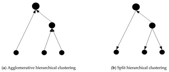
Figure 3. Hierarchical clustering.

The three clustering methods are compared, and the advantages and disadvantages are identified (Table 2). K-means cluster analysis is simple, easy to implement, highly efficient, easily calculated, scalable, and has superior characteristics [27]. Thus, it is the analytical technique applied in the current study.

Table 2. Comparison of clustering algorithms.

Clustering Method	Advantage	Disadvantage
K-means Clustering	Simple, fast, scalable, and efficient	Easily enters a local convergence regime [28]
Density Clustering	Can find clusters of any shape	Sensitive to defined parameters, different parameters lead to different clustering results
Hierarchical Clustering	a. Does not require a predetermined number of clusters b. Not sensitive to the order of input data [29]	a. Cannot undo an existing operation b. Good merging or split operation [30] is difficult to define

2.2.3. Simulation Method

To better analyze the consequences of different insertion angles of vehicles, the PC-Crash software is used to perform vehicle collision experiments. The software uses motion force momentum conservation and energy conservation to determine the accident process and analyze the collision severity of the vehicle. The most direct collision parameters selected are the vehicle collision depth and the total deformation energy of the vehicle, which are relatively intuitive parameters. The collision parameters of vehicles at different angles can generally reflect the impact of the different insertion angles of the vehicles on other vehicles on the road. The reason for this is that the vehicle collision data reflect the worst response to vehicle lane changing.

To improve the analysis of the relationship between the collision angle and the severity of the accident, collision experiments with different insertion angles were conducted using PC-Crash. In the simulation experiment, a Toyota Camry 2.2 vehicle (red vehicle 1) was used to collide with a BMW 130i vehicle (blue vehicle 2). Figure 4 presents the vehicle collision screen.

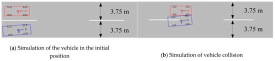
Figure 4. Simulation experiment chart.

2.3. Data Analysis

2.3.1. Vehicle Speed Analysis

The amount of traffic on the road changes at any time during the day. The speed of the vehicle is also affected by numerous factors, such as traffic volume, driver characteristics, and external interference, hence the continuous fluctuation of speed. Changes in speed caused by external environmental interference when the vehicle shifts lanes also vary. The speed of the target vehicle inserted into the target lane exhibits three main changes.

As shown in Figure 5a, when the target vehicle is inserted into the target lane, the speed decreases. Owing to the influence of the target lane, the target vehicle passes the other vehicle after entering the boundary and waiting for the target lane; it then inserts itself into the target lane after the car behind in the target lane passes.

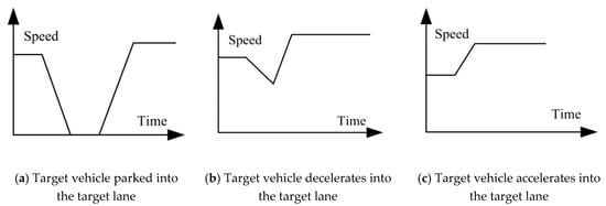
Figure 5. Diagram of change in the speed of the inserted vehicle.

The target vehicle shown in Figure 5b is slowed down by the target vehicle before it is inserted into the target lane; it is then quickly inserted into the target lane at a higher speed.

As shown in Figure 5c, the front and rear vehicles in the target lane have a large gap, and the target vehicle is quickly inserted into the target lane at a high speed.

To better analyze the change in vehicle speed when the vehicle changes lanes, the target vehicle coordinates, as well as the speed of the front and rear vehicles in the target lane are extracted using Tracker. Abnormal points in the data are extracted using the Tracker software; thus, we use the mean method to correct the abnormal points and thus make the original data smoother. After screening the survey data, 5607 data points were selected for tracking the same data. The correlation of the three vehicles was then analyzed using SPSS 2.0. Table 3 shows that the correlation between the speed of the target vehicle in the target lane and the speed of the vehicle in front in the target lane is 0.553 **, and the correlation between the speed of the vehicle behind in the target lane is 0.474 **.

Table 3. Speed correlation analysis.

Target Vehicle Speed	Index		TVIS	TLFVS	TLRVS
	Pearson Correlation		1	0.553 **	0.474 **
	Covariance		1.698	1.073	0.838
	Deviation		0	0	0.001
	Standard Error		0	0.019	0.016
	95% Confidence Interval	Upper limit	1	0.515	0.444
		Lower limit	1	0.591	0.506

Notes: TVIS, Target Vehicle Insertion Speed (m/s); TLFVS, Target Lane Front Vehicle Speed (m/s); TLRVS, Target Lane Rear Vehicle Speed (m/s); ** p < 0.01.

When the target vehicle is inserted into the target la ne, its running speed is restricted by the running speed of the target lane, and the trend of its speed change is similar to that of the target lane. The running speed of the rear vehicle in the target lane is affected by the target vehicle. The change in speed of the rear vehicle lags behind the change in speed of the inserted vehicle.

As shown in Figure 6a, when the target vehicle is inserted into the target lane, the change in speed of the target vehicle is similar to that of the front vehicle in the target lane. The difference in speed for 87.9% of the samples is between −2 and 2 m/s.

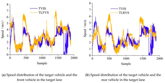
Figure 6. Speed change analysis.

As shown in Figure 6b, when the target vehicle is inserted into the target lane, the speed of the rear vehicle in the target lane lags behind that of the target vehicle, with a lag time. The change in speed of the target lane and the target vehicle is similar to the vehicle-following model proposed by Newell [31].

2.3.2. Analysis of the Distance between the Front Vehicle and Rear Vehicle in the Target Lane

Vehicle spacing is the distance between two cars in the same lane. Large vehicle spacing means a large safety distance between vehicles, low traffic density on the road, and relatively safe vehicle operation. Small vehicle spacing means that the safety distance between vehicles is small, and road traffic density is high. An emergency may cause traffic accidents. In [32], it is indicated that the minimum safe distance between two cars is 2.0 m. Vehicle insertion at a small angle between the last two cars that are moving is difficult to accomplish when the safety distance of the last two cars is less than 2.0 m. For improved analysis of the vehicle data, the plane two-dimensional Cartesian coordinates are constructed, and the vehicle moves along the X-axis, perpendicular to the direction of travel, which is the Y-axis. When the target vehicle is inserted into the target lane, the change in the distance between the target vehicle and the front vehicle and that between the front vehicle and the rear vehicle in the X- and Y-axes of the target lane is analyzed.

As shown in Figure 7, the motion trajectory of the three vehicles exhibits a disordered state. In Figure 7a, the ordinates of the different target vehicles are larger, but the trend is almost the same because the target car shifts from its original lane to the adjacent lane when changing lanes, resulting in a large change in the ordinate. After the lane change is completed, the target vehicle is in the target lane. It continues to move with a slight change in the ordinate. The changes in vehicle trajectory in Figure 7b,c are disordered. However, as shown in Figure 7c, some vehicle ordinates decrease and then tend to be stable. This situation indicates that when the target vehicle is inserted into the target lane, the driver of the rear vehicle in the target lane tends to subconsciously hit the steering wheel to prevent collision with the target vehicle, thereby decreasing the ordinate of the rear vehicle in the target lane.

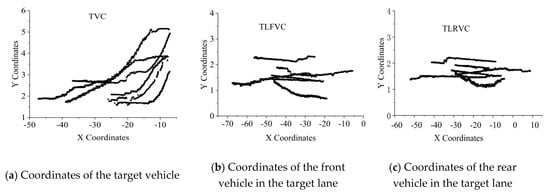
Figure 7. Coordinates of the vehicle captured on video.

Table 4 shows that the p-value of the X-coordinates of the target vehicle and the front vehicle in the target lane is 0.998 **, and the p-value of the X-coordinate of the rear vehicle in the target lane is 0.997 **, both of which show high correlation. The p-value of the Y-coordinates of the target vehicle and the front vehicle in the target lane is 0.090 **, and the p-value of the Y-coordinate of the rear vehicle in the target lane is 0.046**, both of which exhibit high correlation. The analysis indicates that the target vehicle is affected by the coordinates of the front and rear vehicles in the target lane when it is inserted into the target lane.

Table 4. Correlation of the coordinates of the three vehicles.

Target Vehicle X/Y Coordinates			TVC		TLFVC		TLRVC
			X	Y	X	Y	X	Y
	Pearson Correlation		1	1	0.998 **	0.090**	0.997 **	0.046 **
	Covariance		1164.900	0.705	1164.602	0.031	1174.569	0.01
	Deviation		0	0	0	0.001	0	0.001
	Standard Error		0	0	0	0.021	0	0.019
	95% Confidence Interval	Upper limit	1	1	0.998	0.046	0.996	0.009
		Lower limit	1	1	0.998	0.132	0.997	0.086

Notes: TVC, Target Vehicle Coordinate; TLFVC, Target Lane Front Vehicle Coordinate; TLRVC, Target Lane Rear Vehicle Coordinate; ** p < 0.01.

Figure 8a shows that the X-coordinates of the three vehicles exhibit the same trend. When the x-coordinate of the front vehicle in the target lane changes, that the target vehicle and the rear vehicle also change, which conforms to the characteristics of traffic flow propagation. Figure 6 also shows that the target vehicle intersects the front lane trend line of the target lane because the target vehicle accelerates before the lane change; in addition, the vehicle behind the left or right rearward vehicle becomes the preceding vehicle.

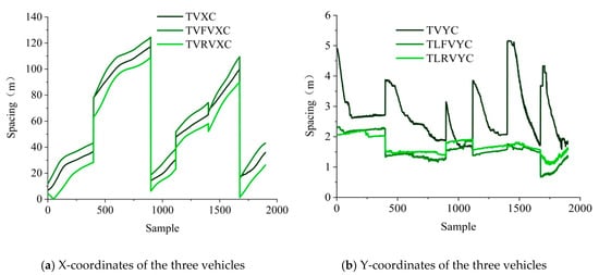
Figure 8. X- and Y-coordinates of the three vehicles.

As shown in Figure 8b, the change in the ordinate of the target vehicle is apparent because the target vehicle shifts from its own lane to the adjacent lane, resulting in a large longitudinal span of the ordinate. After the target vehicle shifts lane, it travels forward under the condition that the Y-coordinates basically remain unchanged, and the front and rear vehicles maintain a certain safe distance. Vehicle coordinates change consistently with the characteristics of the following vehicles.

2.3.3. Insertion Angle of the Target Vehicle

The insertion angle of the lane-changing target vehicle is related to the characteristics of the driver, the running speed of the vehicle, and the insertion distance of the target lane. This study only considers the characteristics of the target vehicle, as well as the characteristics of front and rear vehicles in the target lane. Figure 9 presents the results of the analysis of the acquired samples: the smallest insertion angle is 1.98°, the maximum insertion angle is 56.81°, and the number of samples with an insertion angle below 30° comprises 90.05% of the total sample.

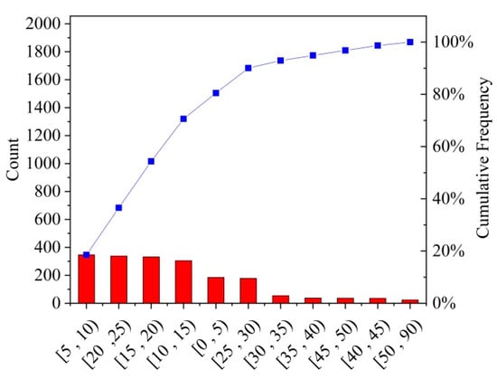
Figure 9. Angle of vehicle at insertion into the target lane.

3. Results

3.1. Classification of the Insertion Angle of the Target Vehicles

K-means clustering is used to group the sample data related to the angle of the target vehicle at insertion. These data are classified into 5 categories. The data in Table 5 show that as the clustering angle increases, the number of cluster samples decreases. The clustering group of the insertion angle of the target vehicle shows that the first three groups of cluster samples comprise 89.56% of the total number of samples, whereas the latter two cluster samples comprise 10.43% of the total number of samples. These results indicate that the target vehicle has 89.56% of the insertion angle of the vehicle at about 23° and below when the target vehicle is inserted into the target lane.

Table 5. Clustering based on vehicle angle.

Number of Groups	1	2	3	4	5
Insertion Angle	6.122	14.763	23.263	34.372	49.438
Number of Samples	556	552	566	84	111
Proportion	29.75%	29.54%	30.28%	4.49%	5.94%

3.2. Insertion Angle of the Target Vehicle and Vehicle Spacing in the Target Lane

The insertion angle of the target vehicle is related to the distance between the front and rear vehicles in the target lane. It is difficult to find the regularity by statistically describing the insertion angle of the target vehicle and the distance between the front and rear vehicles in the target lane. Figure 10a shows the distribution of the insertion angle of the target vehicle, as well as the spacing of the front and rear vehicles in the target lane. To analyze the relationship between the insertion angle of the target vehicle and the spacing in the target lane, the insertion angles of the target vehicle are arranged in ascending order. The insertion angle of the target vehicle is related to the product of the spacing of the front and rear vehicles in the target lane. Figure 10b shows the trend of the fitted curve.

$$y=133.04{{\displaystyle e}}^{\left(x/1572.72\right)}-83.88$$

(5)

where x is the product of the insertion angle of the target vehicle and the spacing of the front and rear vehicles in the target lane. The goodness-of-fit of Formula (5), R² = 0.773, indicates that the data fit well.

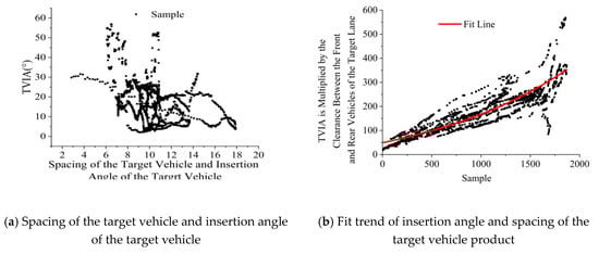
Figure 10. Relationship between insertion angle and spacing.

3.3. Insertion Angle and Speed of the Target Vehicle

The insertion angle of the target vehicle can reflect the smoothness of the lane change of the target vehicle. Under normal circumstances, the insertion angle of the vehicle is below 5° [8]; however, in the nearly saturated state (saturation degree is 0.85–0.95) in a fast-road segment, the vehicle spacing is smaller than the vehicle spacing in a free-flow state, hence the large angle of vehicle insertion into the target lane. Analysis of the survey sample indicates that the change in speed of the target vehicle is not apparent when the target vehicle is inserted into the target lane at different insertion angles. Figure 11 shows the change in the insertion angle of the target vehicle and its speed.

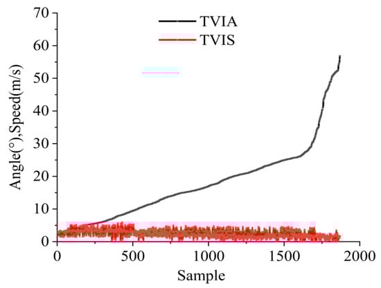
Figure 11. Insertion angle of the target vehicle and corresponding speed.

Figure 12 presents an enlarged view of the speed trend in Figure 11 and shows that as the insertion angle of the target vehicle increases, the speed of the target vehicle decreases.

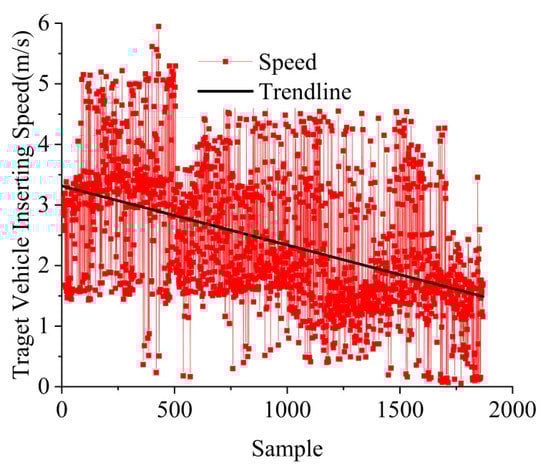
Figure 12. Speed trend of the inserted vehicle.

3.4. Analysis of the Insertion Angle, Speed and Spacing

The insertion angle of the target vehicle is related to the running speed of the target vehicle and the distance between the front and rear vehicles in the target lane. The relationship between the three has yet to be determined. A three-dimensional map is constructed, displaying the insertion angle of the target vehicle, the target vehicle speed, and the distance between the front and rear vehicles in the target lane. Figure 13 shows that the speed of the target vehicle is mainly concentrated in the 0–6 m/s range, the distance is mainly distributed in the 6–14 m range, and the insertion angle is mainly distributed below 30°. K-means clustering is used to group the following data: insertion angle of the target vehicle, speed of the target vehicle, and distance between the front and rear vehicles in the target lane. Table 6 presents the clustering results.

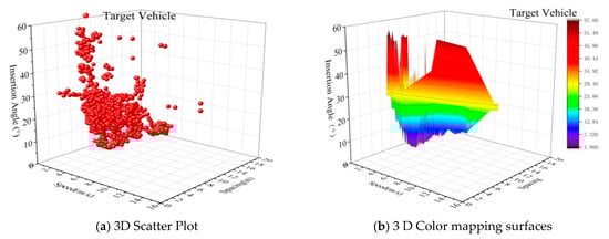
Figure 13. 3 D illustration of the insertion angle of the target vehicle, speed of the target vehicle, and distance between the front and rear vehicles.

Table 6. Clustering results for the speed of the target vehicle, angle of insertion of the target vehicle, and spacing between the front and rear vehicles in the target lane.

Number of Groups	1	2	3	4	5
Speed	3.136	2.450	2.063	1.565	1.211
Space	11.911	10.095	9.970	8.167	7.888
Angle	6.119	14.859	23.348	34.238	49.438
Number of Samples	555	567	550	86	111
Proportion	29.70%	30.34%	29.43%	4.60%	5.94%

Table 6 lists five clusters classified by k-means clustering. The speed, space, and angle of each cluster are given. When the spacing between the front and rear vehicles in the target lane decreases, the speed of the target vehicle decreases, whereas the insertion angle of the target vehicle increases. The insertion angle of the target vehicle comprises 89.47% in the first three groups. The speed range corresponding to the insertion angle of the first three groups of vehicles fluctuates from 2 to 3 m/s and its vicinity. The corresponding spacing ranges from 10 to 12 m. Both the range and its vicinity fluctuate.

3.5. PC-Crash Simulation

Vehicles collide at different angles during lane change collisions. To explain the vehicle collision angles in detail, the collision angles are divided into 11 groups with an interval of 5° between each group. Table 7 lists the total deformation energy, the collision momentum, and the average collision depth of the vehicle at different collision angles.

Table 7. Vehicle insertion collision angle and collision energy statistics.

Collision Angle (°)	Collision Contact Moment (s)	Total Deformation Energy (J)	Impact Momentum (Ns)	Average Collision Depth (mm)
5	11.37	2.38	36.41	15
10	5.04	10.09	77.54	20
15	3.18	26.64	121.85	20
20	2.21	44.52	174.14	25
25	1.65	72.96	232.71	30
30	1.31	108.64	296.81	40
35	1.07	149.57	326.89	40
40	0.9	193.74	428.99	40
45	0.8	237.68	489.96	45
50	0.74	275.96	535.57	45
55	0.69	303.39	555.71	45

Figure 14 shows that the total deformation energy, collision momentum, and average collision depth of a collision vehicle increase as the collision angle increases, with the collision speed remaining constant. When the vehicle collision angle is larger than 30°, the vehicle collision momentum sharply increases; when the vehicle collision angle is larger than 25°, the vehicle collision depth increases rapidly. Therefore, when the vehicle collision angle is less than 25° and the speed remains the same, the total deformation energy, the collision momentum, and the average collision depth of the vehicle are relatively small. Thus, when changing lanes, the vehicle can keep the insertion angle lower than 25°.

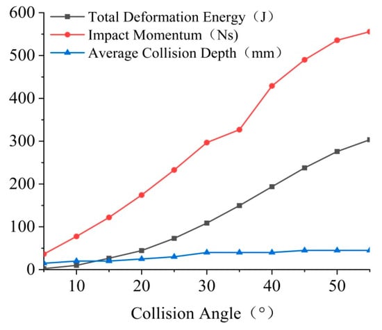
Figure 14. Damage corresponding to different collision angles.

4. Discussion

After the vehicle insertion angles are analyzed, 89.47% of the vehicle insertion angles into the target lane are at or below 23°. To verify the rationality of the insertion angle, we assume that vehicles encounter traffic collisions at different insertion angles. The collision parameters are used to determine the reasonable insertion angle. The lesser the severity of the collision, the more reasonable the corresponding insertion angle. The severity of collision increases as the insertion angle increases.

The angle of the lane-change conflict is 30°–85°, as determined using the conflict angle division method employed by the United States Federal Highway Administration in its micro-simulation modeling of vehicle trajectories. The automatic identification software Surrogate Safety Assessment Model or SSAM was used [33].

Xiang et al. [34] defined the rear-end collision of the same vehicle. When the collision angle is in the 0°–45° range, the vehicles approach each other, demonstrating a collision between the front of the vehicle and the tail of the preceding vehicle.

Owing to the scarcity of vehicle–vehicle small-angle side impact test data, the collision data of the reference vehicle and the guardrail are further used to determine the vehicle collision angle. The Safety Performance Evaluation Standard for Highway Fences—2013 [35] stipulates that the angle of the vehicle collision barrier is 20°.

Table 8 compares different studies, including the current study.

Table 8. Research summary.

Unit/Researcher	Collision Angle/Insertion Angle
United States Federal Highway Administration [33]	30°–85°
Xiang et al. [34]	0°–45°
Safety Performance Evaluation Standard for Highway Fences—2013 [35]	≤20
Bhadeshia [15]	5
This Article	≤23

5. Conclusions

This study analyzes the relationship between the insertion angle of the target vehicle, the speed of the target vehicle, as well as the spacing between the front and rear vehicles relative to the target vehicle inserted into the target lane. To verify the reasonable insertion angle of the target vehicle, we conduct a simulation of the total deformation energy, vehicle collision momentum, and average collision depth of the vehicle under different collision angles by using PC-crash. The main results are as follows:

• For 89.47% of the vehicles, the clustering angle is less than 23°, which is in accordance with the Safety Performance Evaluation Standard for Highway Fences—2013 [35] (less than 20°), indicating that this study is reasonable.
• When the target vehicle is inserted into the target lane, the front vehicles in the target lane, the target vehicle, the rear vehicles in the target lane still follow the car following theory.
• On the basis of the vehicle collision simulation data, as the collision angle of the vehicle increases, the severity of the collision gradually increases, requiring the vehicle to change lanes at a small angle.
• The lane change of vehicles with an insertion angle of 23° or less conforms to the insertion angle of 89.64% of the vehicles. To maintain the safety of lane changing, the vehicle insertion angle should be limited to 23° or smaller.

By determining the insertion angle and speed of the target vehicle, as well as the front and rear vehicle spacing in the target lane, it is proposed that when the road traffic load is 0.85–0.95, the vehicle lane change insertion angle is limited to 23° and below, which meets the requirements of most vehicle lane changes. If a collision occurs at this angle, the impact on traffic is relatively small.

The limitations of this study are as follows: A total of 5607 data points pertaining to 18 vehicles were selected for analysis. Some vehicles cause other vehicles to change lanes at different insertion angles and exert different effects; the different insertion angles determined using different models will be analyzed in further research. Moreover, the characteristics of the driver, which also affect the insertion angle of the vehicle, are not considered. In the collision analysis, only two vehicles were selected to collide at the same speed, subject to certain limitations. In future studies, the insertion angle of the vehicles will be examined in conjunction with the characteristics of the driver. The effects of variations in collision angles at different speeds also need to be verified in further research.

References

- Sun, D.J.; Kondyli, A. Modeling Vehicle Interactions during Lane-Changing Behavior on Arterial Streets. Comput. Civ. Infrastruct. Eng. 2010, 25, 557–571. [Google Scholar] [CrossRef]
- Zheng, Z.; Ahn, S.; Monsere, C.M. Impact of traffic oscillations on freeway crash occurrences. Accid. Anal. Prev. 2010, 42, 626–636. [Google Scholar] [CrossRef] [PubMed]
- Peng, J.S.; Fu, R.; Shi, L.L.; Zhang, Q. Research of Driver’s Lane Change Decision-making Mechanism. J. Wuhan Univ. Technol. 2011, 33, 46–47. [Google Scholar]
- Lee, S.E.; Olsen, E.C.B.; Wierwille, W.W. A Comprehensive Examination of Naturalistic Lane Changers. Available online: https://rosap.ntl.bts.gov/view/dot/4191 (accessed on 28 January 2020).
- Stephens, A.N.; Groeger, J.A. Following slower drivers: Lead driver status moderates driver’s anger and behavioural responses and exonerates culpability. Transp. Res. Part F: Traffic Psychol. Behav. 2014, 22, 140–149. [Google Scholar] [CrossRef]
- Hicks, T.G.; Wierwille, W.W. Comparison of Five Mental Workload Assessment Procedures in a Moving-Base Driving Simulator. Hum. Factors: J. Hum. Factors Ergon. Soc. 1979, 21, 129–143. [Google Scholar] [CrossRef]
- Tian, S.; Xu, K.; Ma, M.N. Lane Changing Behavior of Vehicles in Urban Road Work Zone Based on Cellular Automata. J. Chong Qing Jiao Tong Univ. 2019, 38, 113–118. [Google Scholar]
- National Highway Traffic Safety Administration. Integrated Vehicle-Based Safety Systems: Light Vehicle Field Operational Test, Key Findings Report. Ann. Emerg. Med. 2011, 58, 205–206. [Google Scholar] [CrossRef]
- Gipps, P.G. A model for the structure of lane-changing decisions. Transp. Res. Part B: Methodol. 1986, 20, 403–414. [Google Scholar] [CrossRef]
- Ahmed, K.; Ben-Akiva, M.; Koutsopoulos, H. Models of Freeway Lane Changing and Gap Acceptance Behavior. Transp. Traffic Theory 1996, 13, 501–515. [Google Scholar]
- Kesting, A.; Treiber, M.; Helbing, D. General Lane-Changing Model MOBIL for Car-Following Models. Transp. Res. Rec. J. Transp. Res. Board 2007, 1999, 86–94. [Google Scholar] [CrossRef]
- Ahmed, K.I. Modeling drivers’ acceleration and lane changing behavior. Available online: https://dspace.mit.edu/bitstream/handle/1721.1/9662/42459005-MIT.pdf?sequence=2 (accessed on 29 January 2020).
- Deng, J.H.; Feng, H.H. Multilane Cellular Automation Model Based on the Lane Changing Mechanism. J. Transp. Syst. Eng. Inf. Technol. 2018, 18, 68–73. [Google Scholar]
- Lee, J.; Park, M.; Yeo, H. A probability model for discretionary lane changes in highways. KSCE J. Civ. Eng. 2016, 20, 2938–2946. [Google Scholar] [CrossRef]
- Bhadeshia, H.K.D.H. The first bulk nanostructured metal. Sci. Technol. Adv. Mater. 2013, 14, 14202. [Google Scholar] [CrossRef] [PubMed]
- National Research Council. Highway Capacity Manual 2010; Transportation Research Board: Washington, DC, USA, 2010. [Google Scholar]
- Gazis, D.C. Optimum Control of a System of Oversaturated Intersections. Oper. Res. 1964, 12, 815–831. [Google Scholar] [CrossRef]
- Gazis, D.C.; Potts, R.B. The Oversaturated Intersection. In Proceedings of the 2nd International Symposium on the Theory of Road Traffic Flow, Paris, France, 22 April 1963; pp. 221–237. [Google Scholar]
- Green, D.H. Control of Oversaturated Intersection. Op. Res. Q. 1968, 18, 161–173. [Google Scholar] [CrossRef]
- Yuan, M.; Zhao, X.; Wang, S. Using tracker software to study circular motion in a ferris wheel. Phys. Bull. 2020, 1, 96–98. [Google Scholar]
- Yu, L.; Chen, Q.; Chen, K. Deviation of Peak Hours for Urban Rail Transit Stations: A Case Study in Xi’an, China. Sustainability 2019, 11, 2733. [Google Scholar] [CrossRef]
- He, Q. Advance in Fuzzy Clustering Theory and Application. Fuzzy Syst. Math. 1998, 2, 89–94. [Google Scholar]
- Macqueen, J. Some Methods for Classification and Analysis of Multivariate Observations. Available online: https://www.cs.cmu.edu/~bhiksha/courses/mlsp.fall2010/class14/macqueen.pdf (accessed on 29 January 2020).
- Wu, Y.; Yang, K.; Zhang, J.Z. Using DBSCAN clustering algorithm in spam identifying. In Proceedings of the 2nd International Conference on Education Technology and Computer, Shanghai, China, 22–24 June 2010; pp. 398–402. [Google Scholar] [CrossRef]
- Ester, M.; Kriegel, H.P.; Sander, J.; Xu, X. A density-based algorithm for discovering clusters in large spatial databases with noise. In Proceedings of the 2nd International Conference on Knowledge Discovery and Data Mining, Portland, OR, USA, 2 August 1996; pp. 226–231. [Google Scholar]
- Lin, C.; Yang, Z.; Xi, T. Psychology Dictionary; Shanghai Education: Shanghai, China, 2003; p. 12. [Google Scholar]
- Lin, L.; Chen, J.; Qu, D.Y.; Hei, K.X. Study on traffic state identification method based on K-means clustering algorithm. J. Qingdao Univ. Technol. 2019, 4, 40. [Google Scholar]
- Wang, F. Image segmentation algorithm based on AHLO and K-means clustering. J. Shenyang Univ. Technology. 2019, 7, 41. [Google Scholar]
- Guha, S.; Rastogi, R.; Shim, K. Cure: An efficient data clustering algorithm for large databases. In Proceedings of the ACM-SIGMOD 1998 International Conference on Management of Data, Seatle, WA, USA, 2 June 1998; pp. 73–84. [Google Scholar]
- Duan, M. Research and Application of Hierarchical Clustering Algorithm; Central South University: Changsha, China, 2009; p. 8. [Google Scholar]
- Newell, G.F. A simplified car-following theory: A lower order model. Transp. Res. Part B: Methodol. 2002, 36, 195–205. [Google Scholar] [CrossRef]
- Wang, W.; Guo, X. Traffic Engineering; Southeast University Press: Nanjing, China, 2000; p. 9. [Google Scholar]
- Sun, L.; Li, Y.P.; Qian, J.; Yu, Y. Evaluation of weaving sections with respect to traffic safety based on traffic conflict technique. China Saf. Sci. J. 2013, 23, 55–60. [Google Scholar]
- Xiang, Q.J.; Lu, J.; Lu, C. Road Traffic Conflict Analysis Technology and Application; Beijing Science Press: Beijing, China, 2008; p. 7. [Google Scholar]
- Beijing Traffic Engineering Co., Ltd., Shenzhen Branch. Standard for Safety Performance Evaluation of Highway Barries; Department of Transportation: Beijing, China, JTG B05-01-2013.
© 2020 by the authors. Licensee MDPI, Basel, Switzerland. This article is an open access article distributed under the terms and conditions of the Creative Commons Attribution (CC BY) license (http://creativecommons.org/licenses/by/4.0/).