1. Introduction
As cleaner alternatives to fossil fuel-based vehicles (FFVs), electric freight vehicles (EFVs) have been widely used in logistics and transportation to deal with environmental challenges. Compared with conventional FFVs, EFVs are cleaner and quieter, which means less air pollution and noise. According to the US Department of Energy (DOE), EFVs can reduce greenhouse gas emissions by 48% compared to the traditional FFVs running on gasoline and diesel [
1]. In order to reduce greenhouse gas emissions and improve fuel efficiency, governments have taken corresponding measures to support EFVs. The U.S. National Petroleum Council has confirmed that electric vehicles are a very promising tool for reducing urban air pollution [
2]. Europe is committed to reducing its greenhouse gas emissions by 40% until 2030 [
3]. In the USA, the maximum tax credit for electric vehicles at the national level is
$7500, and states can adopt further incentives to facilitate increased purchases [
4]. The U.S. Environmental Protection Agency (EPA) together with the National Highway Traffic Safety Administration (NHTSA) has adopted measures to promote clean-energy vehicles [
5]. In 2013, the cabinet of the State Council of China approved the Energy Saving and New Energy Vehicle Industry Development Plan, aiming to sell five million battery-powered electric vehicles and plug-in hybrids by 2020 [
6]. China usually provides exemptions from purchase taxes and consumption taxes based on engine displacement and the sales price [
7]. In addition, the Ministry of Industry and Information Technology (MIIT) of China issued the “Interim Regulations on the Traceability Management of New Energy Vehicle Power Battery Recycling” in July 2018, with a special emphasis on battery traceability management. Chevrolet also established an energy storage station using used electric vehicle batteries at the General Motors plant in Michigan [
8]. In Europe, Tesla has cooperated with Umicore to start recycling [
9]. After considering the governmental subsidies that are available for electric vehicles and the high external cost imposed by regulators on pollution and noise, more and more firms have adopted EFVs in their logistics operations, such as FedEx, UPS and JD [
10,
11,
12].
Traditional vehicle routing problems (VRPs) [
13] usually only consider economic performance, and their optimization objective is to minimize the distance, usage time or cost. In the context of sustainability development, researchers have paid more and more attention towards incorporating air pollution, energy consumption or carbon emissions into vehicle routing problems, such as [
14,
15,
16,
17,
18,
19,
20,
21]. Therefore, in this paper, we specifically employ EFVs in the vehicle routing problem to reduce the environmental impact of transportation. However, there are several issues associated with the usage of EFVs, including high fixed investments, long recharging times, limited driving range and load as well as fewer charging stations. Fortunately, these concerns can be addressed by the promising solution of battery swapping, which replaces a depleted battery with a fully charged one. The process of battery swapping only takes about 10 minutes, which is much more efficient than recharging operations [
22]. Moreover, EFVs that use battery swapping are able to charge a nearly depleted battery at off-peak times with lower electricity prices. In summary, the mode of battery swapping has the advantages of enabling fast charging, high safety and long endurance.
After taking the limited driving range and payload into account, how to plan the delivery routes and swap batteries to serve customers in a timely manner becomes an important research problem. We refer to this as the battery swapping electric vehicle routing problem with energy consumption and carbon emissions (BVRP-EC). In other words, BVRP-EC seeks to optimize the logistics operations in a cost-efficient way while reducing energy consumption and carbon emissions, which increases both economic and environmental performance. The goal of this study is to introduce, formulate and solve BVRP-EC by extending a traditional capacitated VRP with loading capacity limitations, a fixed fleet, a driving range constraint and a battery swapping requirement. Given the locations of the depot, battery swapping stations and customers, the proposed model decides: (1) the number of utilized EFVs; (2) the allocation of customers to each EFV while guaranteeing the driving range and loading capacity limitations; and (3) possible visits of each EFV to the battery swapping stations to fulfill the orders with enough power. At the same time, the routing arrangement of this model should minimize the entire costs consisting of EFVs usage and energy consumption.
We contribute to the existing literature as follows. First, we introduce a comprehensive model to estimate energy consumption and carbon emissions in the EFVs routing problem. This model considers a few internal and external factors, such as speed, weight, travel distance, windward area and road conditions. Second, we study the BVRP-EC and build a corresponding mixed integer programming model. This model differs from traditional VRPs by considering new constraints such as EFV driving range limitations and battery swapping strategies. Third, an efficient algorithm named AGE-HN (adaptive genetic algorithm combing hill climbing and neighborhood search) is proposed to solve BVRP-EC. The crossover and mutation probabilities are designed to adaptively adjust with any changes to the population fitness. Hill climbing search is used to enhance the local search ability of the algorithm. Neighborhood search is created in the algorithm as a post-optimization to make the EFV visit battery swapping stations one or more times while sufficient power is available. Moreover, computational experiments are notably designed to evaluate the performance of AGE-HN.
The remainder of this paper is organized into the following sections.
Section 2 provides a literature review related to the energy consumption of electric vehicles and the electric vehicle routing problem. In
Section 3, we describe the BVRP-EC problem, introduce a comprehensive measurement method of electric vehicle energy consumption and propose a mathematical model for BVRP-EC. In
Section 4, the algorithm of AGE-HN is presented in detail to solve BVRP-EC. We use the computational experiments to test and analyze the algorithm’s performance in
Section 5. Finally,
Section 6 concludes this work and provides several potential research avenues for the future.
3. Model Formulation
3.1. Problem Description
For convenience, we first define some mathematical symbols: a complete directed graph represents the freight distribution network for BVRP-EC, where is the set of nodes; is the set of customer nodes; is the set of battery swapping stations; Node 0 represents the depot—it is assumed that the depot also has a battery swapping station; is the maximum number of available battery swapping stations; is the set of arcs; represents a set of EFVs with the load capacity , and is the maximum number of available EFVs; the distance of each arc is set to be ; is the travel speed of EFVs in arc ; represents the energy consumption of EFVs in arc ; indicates the load carried by the electric vehicle in arc ; the service time of EFVs at the battery swapping station is , ; represents the demand for goods at customer , ; is the battery capacity of EFVs; represents the remaining electricity when the vehicle completes the visit on arc. The decision variables are required in the following: Binary variable is 1 when the vehicle visits arc , otherwise it is 0.
For the problem of BVRP-EC, there is a vehicle fleet of EFVs with a limited number of vehicles, load capacity and battery capacity. There are a set of customers with a deterministic level of demand, a depot and a set of battery swapping stations. Their locations are given and fixed. Each EFV starts from the depot to deliver goods for customers, and then returns to the depot after completing the task. Each customer is visited only once. The battery swapping station can replace depleted batteries with fully charged ones, which takes a much shorter time than the charging mode. We assume that the EFVs have full battery power after they reach the depot and the battery swapping stations. Unlike the traditional vehicle routing problem with FFVs, this assumption usually allows vehicles to visit the customer only once while BVRP-EC takes the battery swapping electric-vehicle as a carrier, which may need to be charged in the battery swapping station. In order to accomplish the delivery task, EFVs are allowed to visit a battery swapping station one or more times.
Meanwhile, the constraints of battery swapping stations and the battery driving range are considered. We define the usage cost of EFVs per hour as , which is positively proportional to driving time, consisting of a driver’s salary, the tolls for crossing the roads and bridges, etc. The battery swapping station collects the fee of the battery swapping service based on the power consumption of EFVs. In this context, we assume that the cost of power consumption is per kilowatt hour. BVRP-EC will optimize the EFVs routing to minimize the total cost of vehicle usage and power consumption. In addition, as discussed above, the following conditions should be satisfied: A battery swapping station can be visited several times by EFVs; the load capacity of each vehicle must exceed the total customer demand in its route; each vehicle only has a one-way trip; and the driving range is limited because of battery capacity.
3.2. Calculation of Energy Consumption and Carbon Emissions of EFVs
There are different perspectives for vehicle energy consumption, such as Well to Wheel (WTW) and Tank to Wheel (TTW) [
40]. The majority of the transportation fuel consumption and emissions use TTW mode, where the fuel loaded by the freight is converted into automobile power. In this paper, we take energy consumption and carbon emissions into account from the perspective of TTW. In logistics operations, the energy consumption of electric vehicles is affected by many factors, such as the speed, acceleration, weight, frontal area, distance and road conditions [
41]. Among them, the dynamic change of vehicle speeds is affected by air resistance and road congestion, which then affects the consumption of electric power. The weight of electric vehicles includes empty weight and load, and the load decreases when the number of customers to be delivered is reduced. Following [
15], the energy consumption of electric vehicles on arc
can be calculated as follows:
where
is a constant related to the road section; parameter
represents vehicle acceleration; parameter
is the gravity constant; the road angle is
and the rolling resistance coefficient is
;
is the weight of the empty electric vehicle;
is the coefficient related to EFVs;
is the traction coefficient;
is the windward area of the vehicle; and
is the air density. The energy consumption calculation method used in this paper can comprehensively reflect the influence of the key factors, such as speed, load and driving distance, which makes the calculation of electric vehicle energy consumption more accurate and consistent with its practical applications.
The carbon emissions of electric vehicles are related to the energy consumption on arc
and the energy emissions factor
of the electric vehicles. Thus, the measurement of carbon emissions is given as follows:
where the electric energy emission factor
is the carbon dioxide emission per unit of electric energy. This factor is related to the type of electric vehicle and power generation and is a constant in a specific logistics distribution. Here, we set it to
= 0.69 kg/kwh [
42,
43].
In reality, due to economic and scientific uncertainties, there are a lot of uncertain factors in the calculation of electric vehicle carbon emissions, such as emission levels, prediction methods, related emission concentrations, temperature levels and so on. All these factors play important roles in the assessment of carbon emission costs [
44]. Furthermore, there are also many uncertain elements that may indirectly affect vehicle carbon emissions by affecting future transportation activities, such as household motorization levels and structures, building costs and so on [
45]. In order to facilitate calculations, we mainly consider some closely relevant factors such as vehicle speed, weight and travel distance, etc. In the future research, taking the uncertainty of carbon emissions into consideration will become one of our critical research directions.
3.3. Models
According to the calculation of EFVs energy consumption and carbon emissions, the mathematical model of BVRP-EC is described as follows:
The objective function (3) minimizes the total costs consisting of the electric vehicle use cost and power consumption cost. Constraints (4) and (5) ensure that each customer node is visited only once. Constraints (6) are the limited depot and the number of vehicles, which means that all EFVs start from the depot and return to it after completing the task. Constraints (7) are the flow conservation equations. Constraints (8) and (9) are the loading capacity of the electric vehicles. Constraints (10) mean that the electric vehicle is fully charged after charging in the battery swapping station. Constraints (11) state that the remaining power consumption after the electric vehicle passes through an arc does not exceed the remaining power consumption on the node minus the power consumption on this arc. Constraints (12) ensure that the electric vehicle has enough residual power to return to the depot. Constraints (13) reflect the binary decision variables.
It can be seen from the objective function of BE-LRP that there are two special cases in this problem. First, let , and this model will minimize the power consumption of electric vehicles. As explained earlier, since carbon emissions are directly proportional to the power consumption of electric vehicles, they are also equivalent to minimizing carbon emissions in transportation. Second, let , and the objective of the model is to minimize the travel time cost in transportation. Therefore, by considering the travel time cost and low-carbon cost of this model, it can reflect comprehensive evaluation of the economic and environmental performance in the distribution of electric vehicles.
The objective function of BVRP-EC considers the total costs of vehicle use and power consumption, while a traditional VRP usually takes the minimum total travel distance as the goal. Meanwhile, BVRP-EC also imposes constraints related to electric vehicle charging, power consumption and a fixed fleet. Moreover, it allows electric vehicles to visit a battery swapping station multiple times so as to satisfy delivery requirements. This also consists with the reality of logistics distribution.
4. Solution Algorithm for BVRP-EC
The classical VRP is a NP-hard problem [
13] and the BVRP-EC is one of its extensions. In order to improve the solution efficiency, it is necessary to design a heuristic algorithm. Therefore, this paper proposes an adaptive genetic algorithm based on hill climbing optimization and neighborhood search (AGE-HN). An adaptive genetic algorithm is an intelligent algorithm whose parameters can be adjusted flexibly according to the search process [
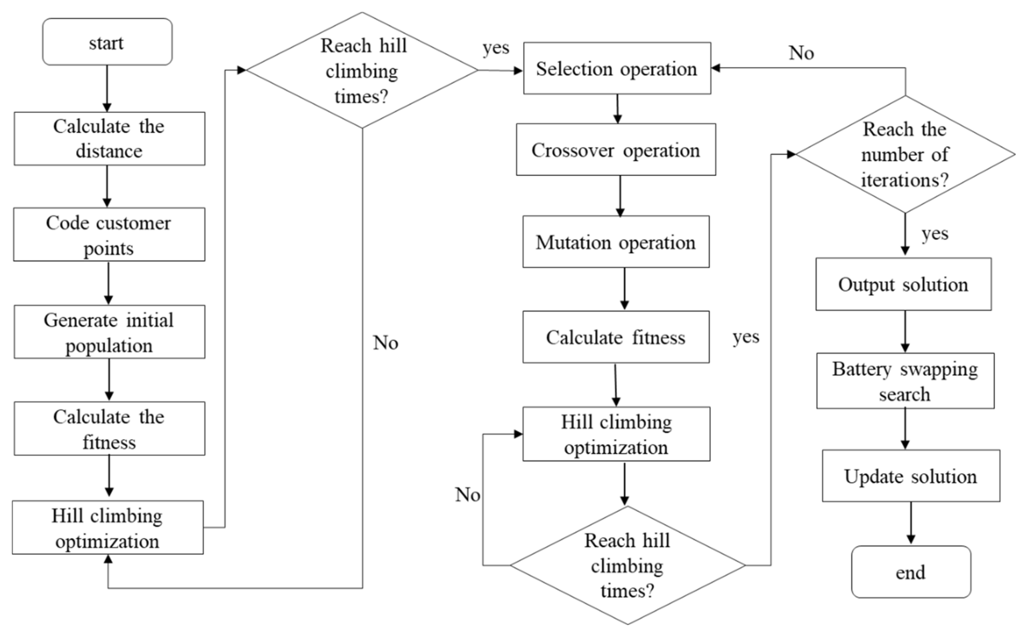
46]. Compared with the classic genetic algorithm, the crossover and mutation probabilities are adaptively adjusted with the population fitness. In order to strengthen the local search ability of the algorithm and ensure the algorithm converges to the optimal solution quickly, this paper also introduces the hill climbing search algorithm. The hill climbing algorithm uses the iteration process to improve the current solution until the solution reaches a “peak”. In addition, in order to meet the constraints of battery range and battery swapping stations, a neighborhood search of the battery swapping stations is carried out for each route in the optimal solution generated by the adaptive genetic algorithm to further improve the optimal solution and finally obtain the optimal feasible solution. The basic flow chart of AGE-HN is shown in
Figure 1.
4.1. Coding, Population Initialization and Fitness Function
Based on the characteristics of the BVRP-EC model, we use a natural number coding strategy. Firstly, we determine the individual chromosome length based on the number of depots, customer nodes and battery swapping stations. Then, individual coding element is added to the EFV routing. The natural number code is expressed as follows: The depot is 0; customer nodes are ; and battery swapping stations are denoted by . We can decide the minimum number of electric vehicles for good delivery in terms of the total demand of all the customer nodes and the EFV’s loading capacity. For example, we can assume that there are 10 customers, and at least 2 vehicles are needed, which is expressed by 2 chromosomes. The number of chromosomes is equal to the number of electric vehicles. The customer service node set of the first vehicle is (3, 4, 5, 6). The position of genes (3, 4, 5, 6) in the chromosome can be arranged randomly. Similarly, the service customer node set of the second vehicle is (7, 8, 9, 1, 2), and the position of genes (7, 8, 9, 1, 2) in the chromosome can be arranged randomly as well. As a result, a complete vehicle routing (0, 3, 4, 5, 6, 0, 7, 8, 9, 1, 2, 0) is created by these two chromosomes via the depot 0.
In the population, each individual corresponds to its own delivery route. The judgment of individual fitness mainly depends on two aspects: (a) Individual objective function value; (b) whether the individual meets the constraints. This paper adopts the natural number coding method, and the encoding process takes the constraints of the problem into account, such as the number of electric vehicles, vehicle load and driving range. In line with minimum value of objective function for BVRP-EC, the fitness function is represented by a maximum value, .
4.2. Selection Strategy
This paper uses a selection strategy combining the best individual and the Roulette method. First, the fitness of each individual is calculated. Second, individuals are ranked in descending order according to their fitness value. Individuals with the highest fitness value are retained to enter the subsequent genetic operation. Finally, the roulette method is used to determine whether the remaining individuals can enter the follow-up operation. The Roulette method calculates the ratio of individual fitness to total fitness in the population, , where is the set of all individuals in the population. The larger the ratio is, the greater is the probability of individual selection.
4.3. Crossover Strategy
The crossover strategy adopted in this paper is to deal with chromosome genes properly and improve the solution space, so as to produce more excellent individuals. It is assumed that , and represent the average fitness, minimum fitness and maximum fitness of the population, respectively. We also set the parameters and . is the ratio of the average fitness to the maximum fitness within the population, which reflects the fitness distribution within the population. The closer the value is to 0.5, the higher the population concentration becomes. is defined as the ratio of minimum fitness to maximum fitness, reflecting the fitness concentration of the whole population. When it gets close to 0, it means that the algorithm may fall into the local optimal solution. On the other hand, when , , this represents a group of individuals with centralized fitness, otherwise the individual fitness of the population is relatively scattered.
The crossover operation can affect the searching ability of the solution space through the operations of the chromosome gene, retaining excellent individuals and producing new ones. In order to avoid premature convergence, inbreeding and inferior individuals harming the population, the following adaptive crossover probability is given:
where
represents the crossover probability,
is the set of individual components of the parent,
and
are the
th component of the parent,
and
are the minimum and maximum components of an individual, respectively, while
and
represent the two fitness levels of the parent.
In the early stage of the algorithm, when the individuals in the population are relatively scattered, there is a large genetic difference among paternal individuals. The higher the fitness of the parent, the greater the probability of crossover operation. In the later stage of the algorithm, the individuals in the population tend to concentrate and there are two situations: (1) The genetic difference between the parents is small and the algorithm may converge to the optimal solution. It is necessary to improve the probability of the crossover operation so the average fitness can further approach the maximum value. (2) Due to the large difference of gene performance among parents, it is easy to lead to a local optimal solution. This means a larger cross probability is needed.
In this paper, we decide whether to use the crossover strategy by judging the relationship between the crossover probability and the generated random real number in (0, 1). The crossover operation is performed only if is greater than this random value, as shown below. (1) Two chromosomes are randomly selected as the parent chromosomes of the crossover operation. (2) For two vehicle routes in the given parent chromosome, the crossover position is randomly selected and the sequential crossover operation is performed. (3) Two new chromosomes are generated by merging the daughter chromosomes of the two vehicle routes and removing the elements with continuous 0 values.
4.4. Mutation Strategy
Mutation operation imitates chromosome mutation in gene inheritance, thus increasing population and chromosome diversity in a solution space. In this paper, the adaptive mutation probability is used to enhance the diversity of individuals and make the algorithm jump out of the local optimal search process as soon as possible. The adaptive mutation probability is calculated as follows:
In the early stage of the algorithm, when the individuals in the population are scattered, the population diversity in the solution space is high and a fixed mutation probability is used. However, in the later stage of the algorithm, the individuals in the population are concentrated and the population diversity in the solution space is low. In this case, the mutation probability is adaptively adjusted according to the fitness. In other words, if the fitness of the individual is greater than the average fitness, the probability of mutation operation decreases with the fitness value, otherwise the probability of mutation operation increases.
In this paper, we first decide whether a mutation operation is carried out by judging whether the adaptive crossover probability is greater than the real number randomly generated in (0, 1). If it is less than the real number, the mutation operation is canceled; otherwise, the following operations are conducted. (1) Following the aforementioned rules, the selected chromosome is regarded as the parent chromosome. (2) In the parent chromosome, the mutation positions of all vehicle routes are determined randomly, and the crossover mutation operation is carried out. (3) The successive 0 elements are deleted and the daughter chromosomes of vehicle routes are merged to generate a new chromosome.
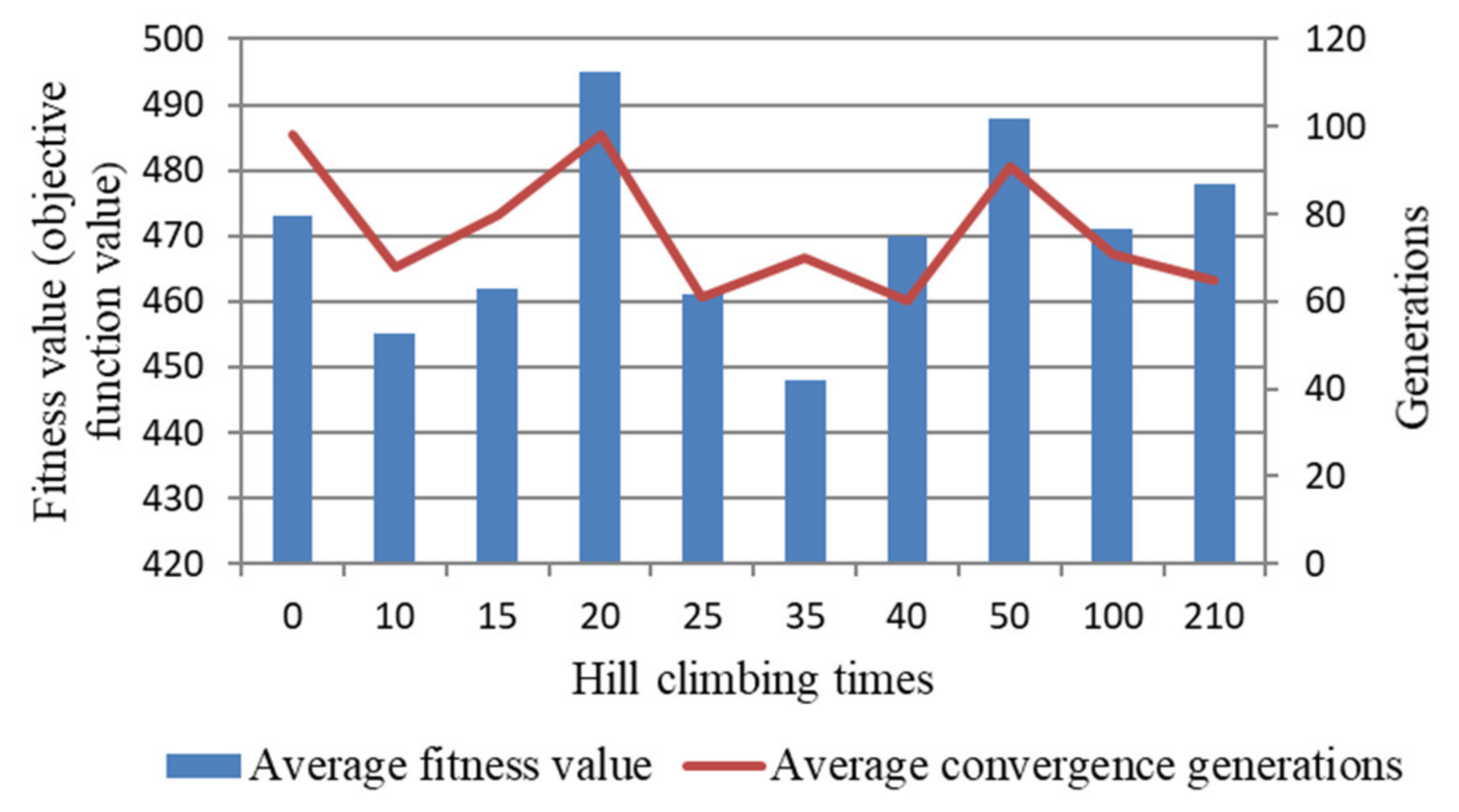
4.5. Hill Climbing Optimization and Termination Criteria
The hill climbing optimization of the algorithm is mainly used in the following two stages. In the first stage, the initial population is optimized and the individual fitness of the population is improved. In the second stage, after the genetic process of the algorithm is executed, the optimal fitness individuals are optimized to realize the local optimization of the optimal solution of the genetic operation and the solution is further improved. The following steps are performed for the hill climbing optimization:
Step 1. For the sub vehicle routes represented by chromosomes, the position of the gene is randomly selected and the crossover operation is performed.
Step 2. The fitness values of each individual before and after the crossover operation are compared. If it becomes larger, then the original chromosome is replaced; otherwise, the original chromosome remains unchanged.
Step 3. Determine whether the termination condition has been reached. If not, repeat steps 1 and 2 until the specified number of iterations is reached.
There are three common types of termination rules. First, when a given objective functions value is reached, the algorithm is terminated. This method usually needs to know the optimal objective value in advance. Second, if the current solution is not improved after several continuous iterations, the algorithm will terminate. Because the number of continuous iterations is difficult to estimate in advance, the algorithm may not be able to jump out of the local optimal solution. Third, based on the required calculation time and accuracy, the maximum number of iterations can be set to ensure that the algorithm converges to the optimal solution. Therefore, this paper selects the third termination rule.
4.6. Neighborhood Search for Battery Swapping Stations
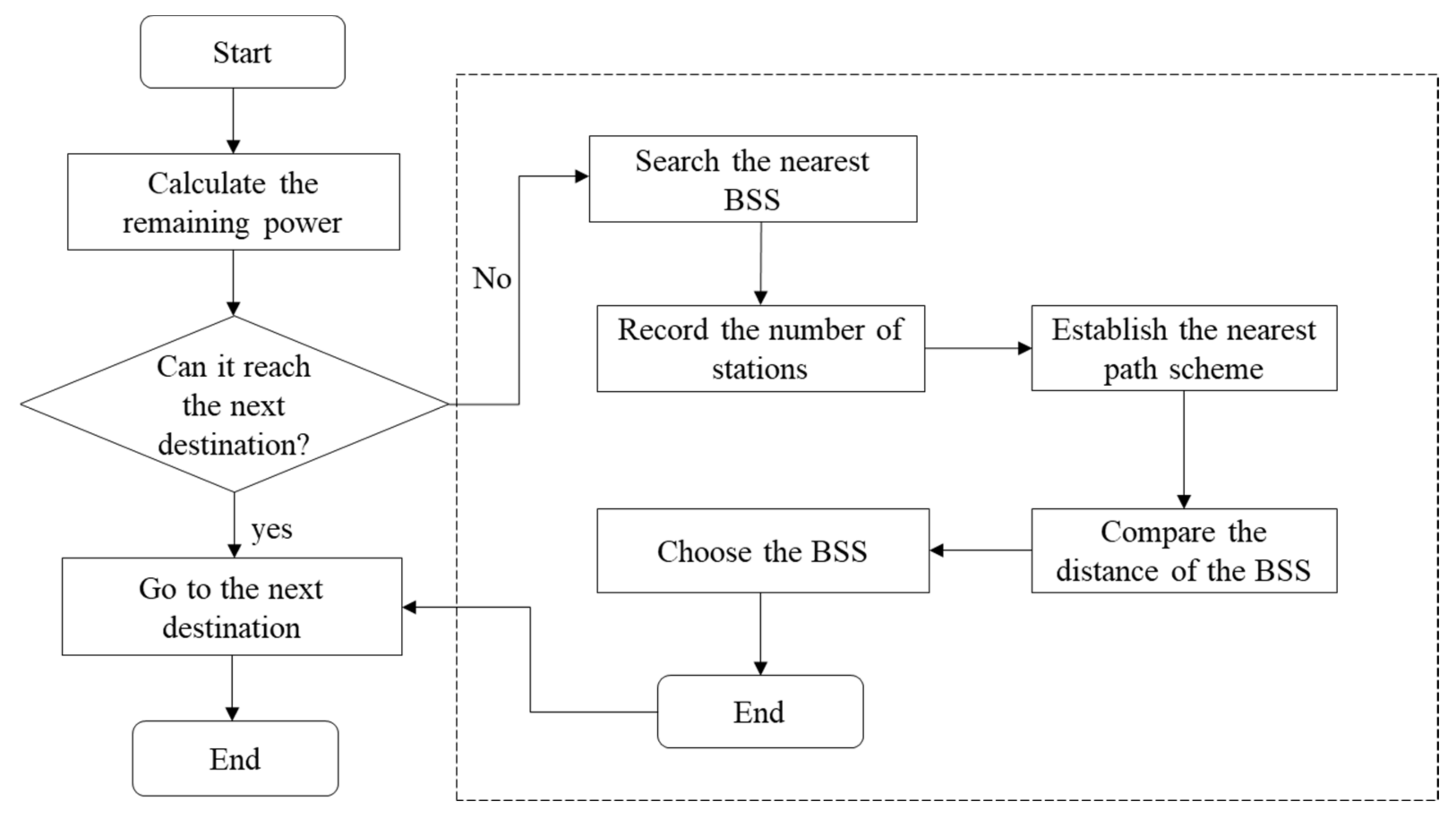
According to the location of the customer nodes and the battery swapping stations, neighborhood search is used to ensure that each route in the optimal solution meets the constraints of battery driving range and battery swapping stations. As the location of the battery swapping stations is given, when the electric vehicle is driven to a customer node in the order of delivery, whether to carry out the battery swapping operation is decided according to whether the remaining power can reach the next customer node or not. If the remaining power is not enough to go to the next customer node, neighborhood search will find the nearest batter-swapping station based on the driving radius between the two customer nodes. The neighborhood search procedure for reaching a possible battery swapping station is shown in
Figure 2.
The detailed steps of the neighborhood search are as follows:
Step 1. Calculate the remaining power once an electric vehicle arrives at a customer node.
Step 2. Judge whether the remaining power can reach the location of the next destination (customer node or depot). If yes, go to step 3; otherwise, go to step 4.
Step 3. Go to the next destination node and terminate the battery swapping search.
Step 4. Find the nearest battery swapping station locations and record the number of battery swapping stations that can be reached.
Step 5. Establish the nearest route scheme. Calculate the distance among the customer node, each battery swapping station and the next destination node.
Step 6. Compare the distance to each battery swapping station, and finally choose the shortest one.
Step 7. Stop the neighborhood search, go to Step 3.
4.7. AGE-HN Algorithm
According to the previous algorithm design and the key steps, the main steps of the AGE-HN algorithm are provided as follows:
Step 1. Set the initial population size as Inn and the maximum number of algorithm iterations as Gnmax. Calculate the distance between each two vertices. Code the individual and generate the initial population which meets the constraints.
Step 2. Calculate the fitness of the initial population and record the individual with lowest fitness.
Step 3. Optimize the individual with the lowest fitness in the population using hill climbing, replace the original individual and set the initial iteration number of hill climbing, .
Step 4. Determine whether the maximum number of climbing optimization Tmax has been reached. If so, record the optimal solution of the current population; otherwise, go to Step 3, set .
Step 5. Rank the fitness level of the current population and calculate the selection probability of each individual. If an individual has the highest fitness in the current population, then the selection probability is set to be 1; for others, the selection probability is determined by the roulette rule. Set the initial iteration number of the algorithm as .
Step 6. Perform a crossover operation: According to the adaptive crossover probability, calculate the crossover probability of each individual. Randomly generate a real value between (0, 1). If the crossover probability is larger than the random value, perform the crossover operation; if the crossover probability is less than the random value, the crossover operation is not used.
Step 7. Perform the mutation operation: calculate the mutation probability of each individual in terms of the adaptive mutation probability. Generate a random real value between (0, 1). If the mutation probability is larger than the random value, perform the mutation operation; otherwise, the mutation operation is not used.
Step 8. Calculate the individual fitness of the new population and record the current individual with highest fitness.
Step 9. Optimize the individual with the highest fitness by using the hill climbing method. If the fitness value is improved, then replace the original individual. When the original value is updated, the iteration times of hill climbing will increase; afterwards, set the initial number, .
Step 10. Determine whether the maximum number of climbing optimization Bmax has been reached. If so, record the optimal solution of the current population; otherwise, go to step 9, set .
Step 11. Judge whether the maximum number of iterations Gnmax is reached. If so, record the current optimal individual and go to step 12; otherwise, go to step 5, .
Step 12. In the optimal solution, perform a neighborhood search for the battery swapping stations, and update the optimal feasible solution.
Step 13. Terminate the algorithm and output the optimal feasible solution.
6. Conclusions
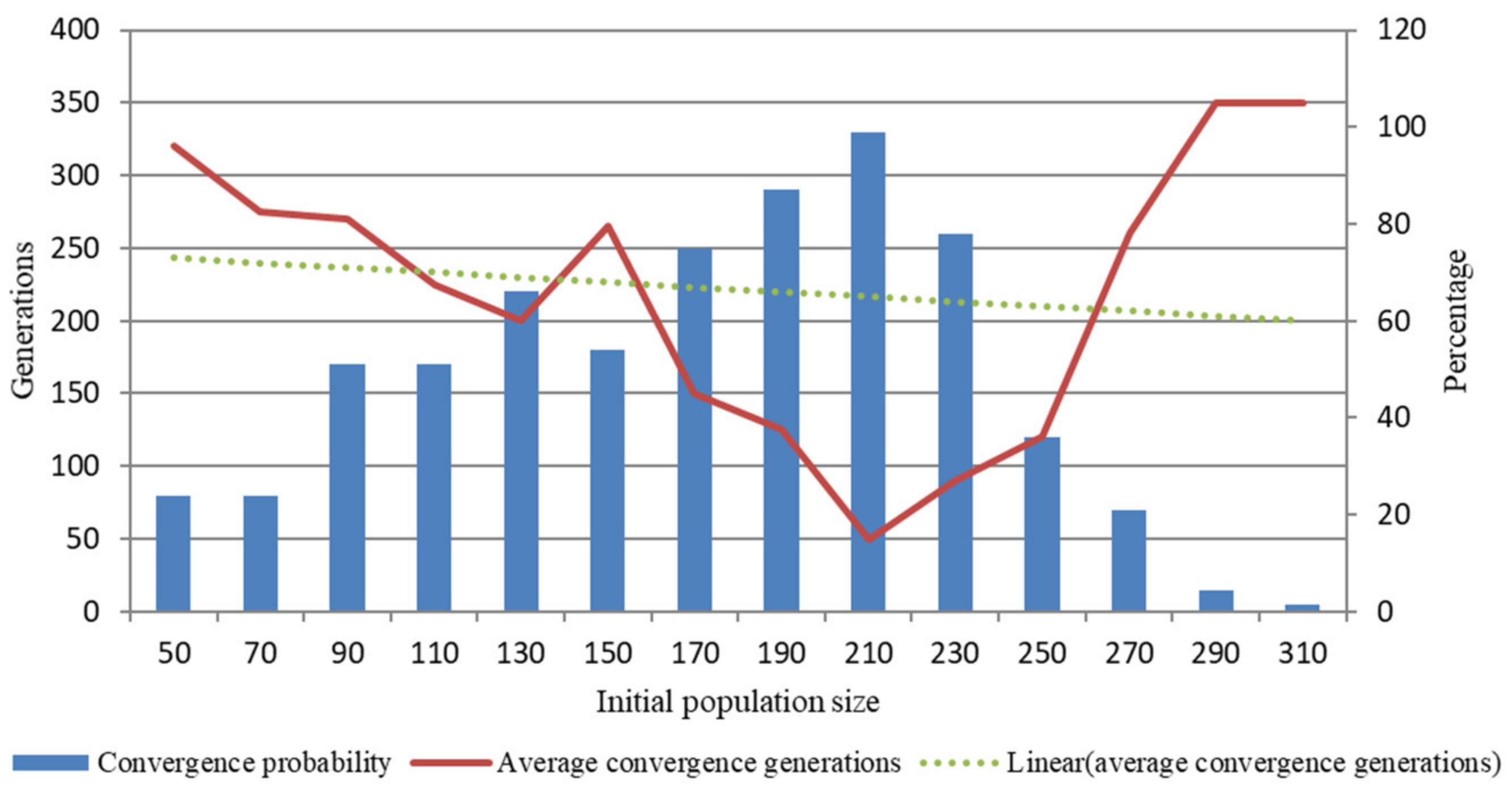
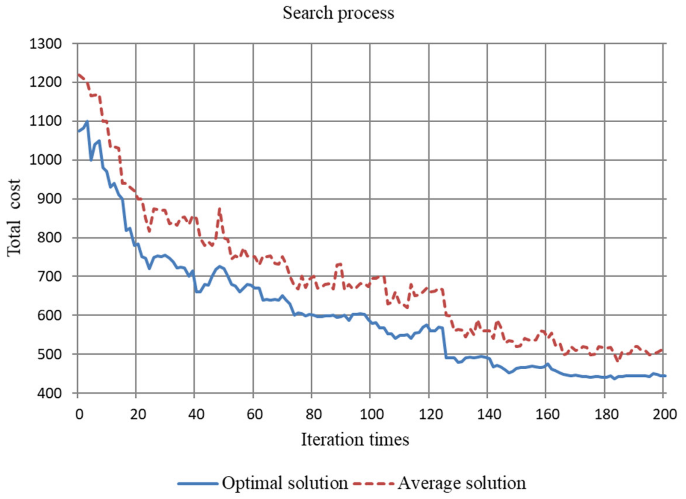
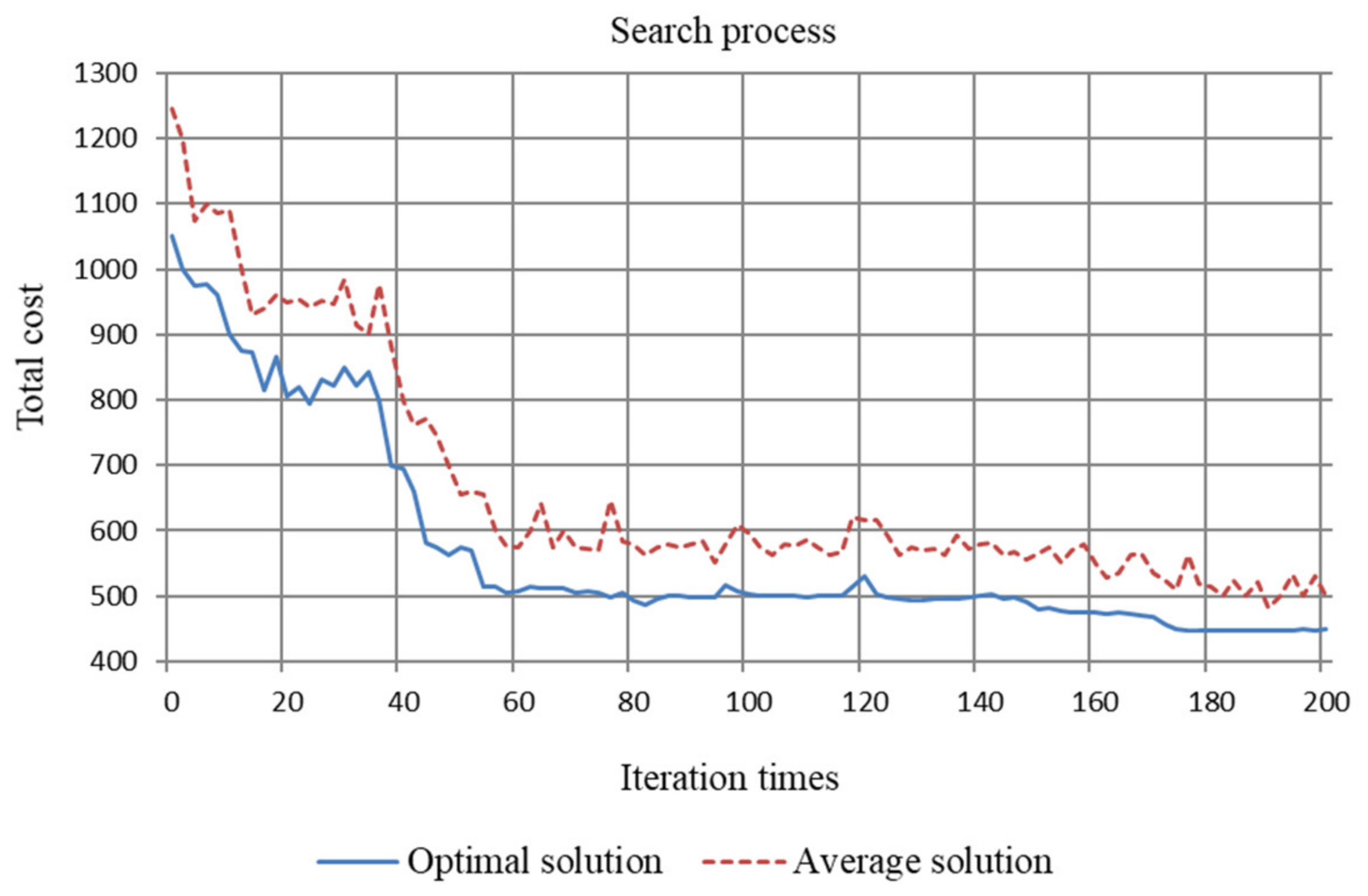
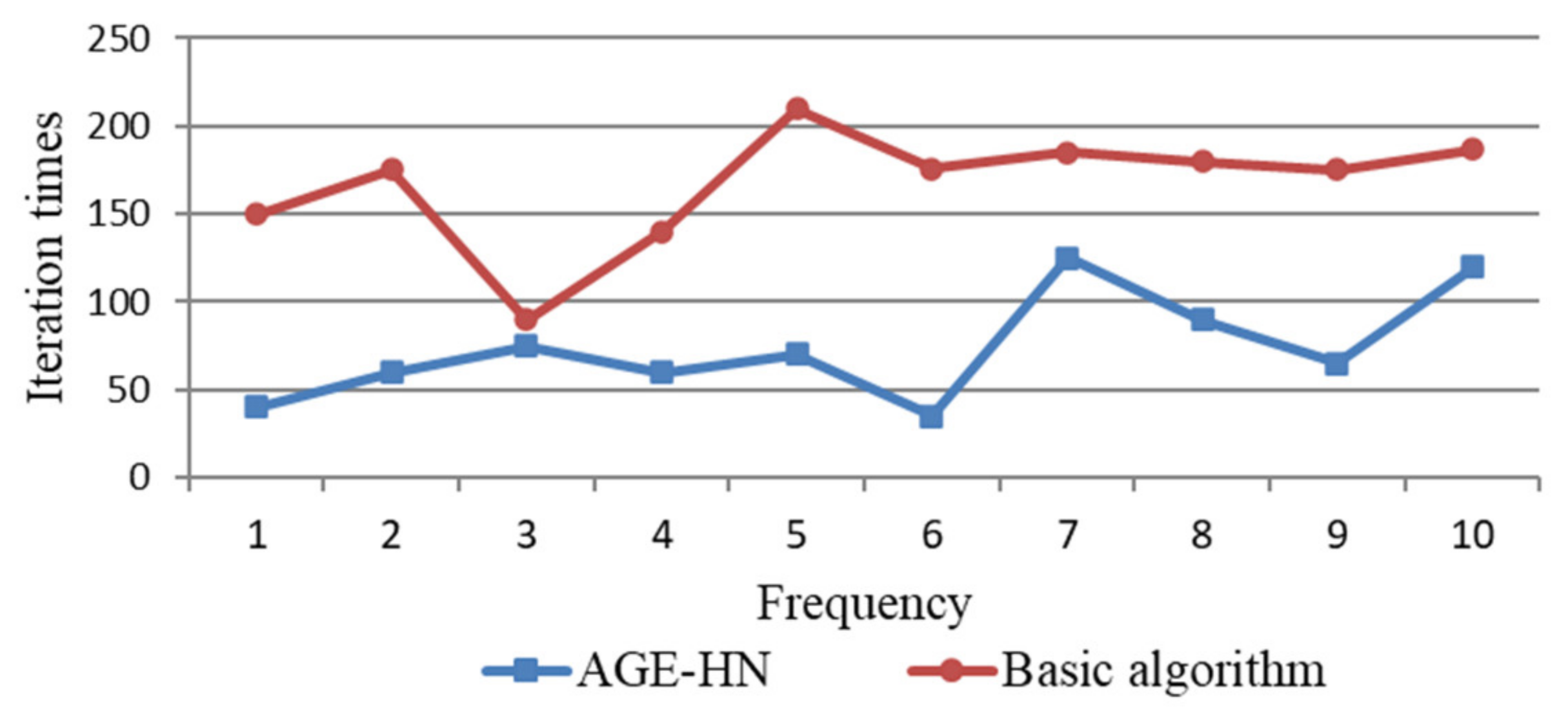
Nowadays, environmental protection has gained public attention all over the world. The development of electric vehicles represents the future of the automobile industry in many countries, such as Japan, the UK and China. Hence, it is of great practical significance to study and analyze logistics transportation based on electric vehicles. Optimizing electric vehicle routing is an important measure to realize energy savings and emissions reduction in logistics delivery. This paper extends the classical VRP to the battery swapping electric vehicle routing problem with energy consumption and carbon emissions (BVRP-EC). To this end, we introduce a comprehensive calculation method of energy consumption and carbon emission of electric vehicles with various factors such as speed, load and driving distance. Moreover, we establish a mixed integer programming model for BVRP-EC. This model considers several new constraints such as electric vehicle capacity, battery range and potentially multiple visits to battery swapping stations. Its objective is to minimize the total costs of the vehicle use and power consumption throughout the delivery. To solve BVRP-EC efficiently, we propose an adaptive genetic algorithm based on hill climbing and neighborhood search (AGE-HN). In this algorithm, the crossover and mutation probabilities are adaptively adjusted with the population fitness. The local search ability of the algorithm is enhanced by hill climbing optimization. In addition, a neighborhood search strategy is proposed to meet the battery range and battery swapping station constraints. Thus, the optimal solution of the model can be obtained. Finally, our numerical experiments show that the adaptive genetic algorithm can quickly and effectively obtain a satisfactory feasible solution to ensure the minimization of economic costs and carbon emissions. Furthermore, our algorithm comparison shows that the proposed adaptive genetic algorithm can converge to the optimal solution faster and improve the efficiency of solving BVRP-EC.
The research results in this paper can provide decision support tools for logistics enterprises using electric vehicles. They can also provide policy insights for the government on electric vehicle logistics. First, the promulgation of some low-carbon policies, such as a carbon tax and a carbon trading mechanism, will be conducive to the promotion of the use of electric vehicles. Second, based on the distribution of depots and customers, the construction of public battery swapping stations will help to improve the battery range of electric vehicles, thus reducing energy consumption and carbon emissions. Finally, due to the strong constraint of battery range, the government should encourage the research and development of advanced battery technologies, so as to get rid of an excessive dependence on charging stations.
On the other hand, our study can also include more practical issues in the future. For example, it is worthwhile to study the electric vehicle routing problem in the context of sharing economy, where social or private freight vehicles may be utilized simultaneously to fulfill delivery aims. In addition, more recently, en route recharging of electric vehicles has attracted attention, where the electric vehicle can be charged while driving [
50]. Therefore, how to extend the driving range in the vehicle routing problem by combing battery swapping and en route recharging modes may be another promising research direction.

 ), customer nodes (
 ) and battery swapping stations (
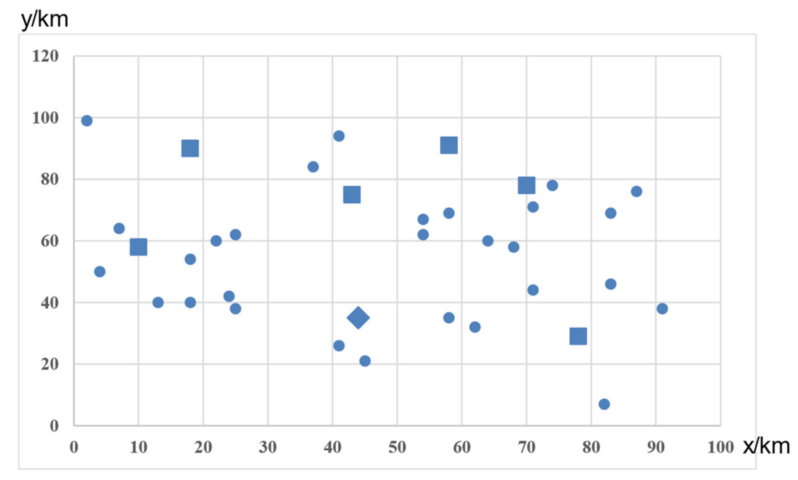
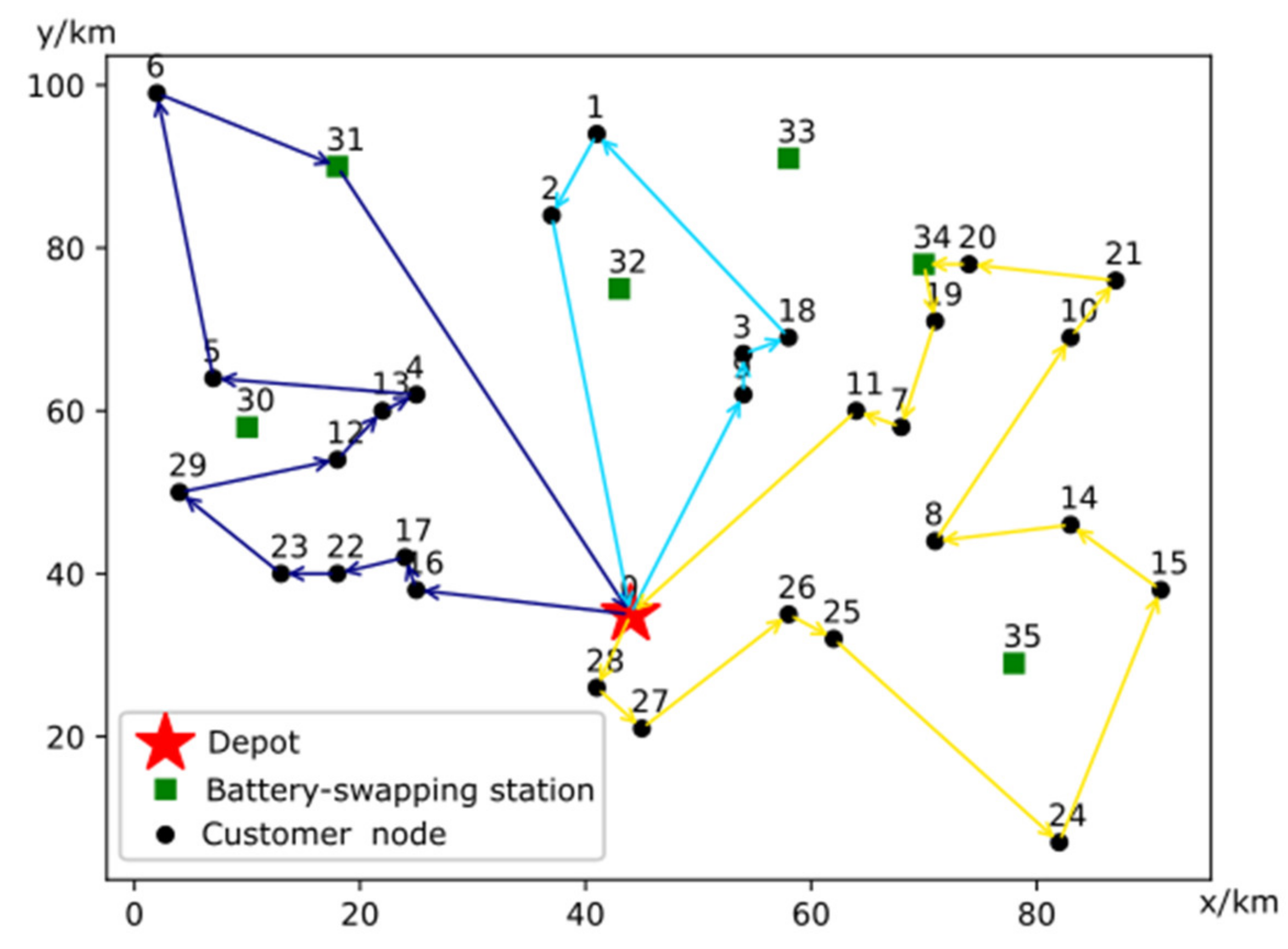
 ) is as shown in Figure 3. In the current electric logistics vehicle market, minivan and light trucks are the main vehicles, accounting for 31% and 19% of the total market, respectively, which are suitable for logistics transit transportation and terminal distribution. After considering the economic cost and practical application, this paper chooses a minivan electric vehicle as the delivery vehicle and uses the industrial electricity price of 0.8 CNY/kWh as the battery swapping cost.


