Sustainable Construction of Earth Dams: Use of Heterogeneous Material from the Dam Site

Abstract

The volumes of soil required for the construction of an earth dam are usually of importance, so that, consequently, a key aspect to mitigate the negative impacts of dam construction, both from an economic and environmental point of view, is the use of materials in the vicinity of the dam location. However, this is often complicated because the existence of good quality materials with homogeneous properties, necessary for the dam core, is scarce in sites near the dam and their presence in sufficient volume for its construction is not usual. Unfortunately, using and transporting soil with good geotechnical characteristics to construct the core in a faraway location is economically and environmentally unsustainable. Therefore, the possibility of using less suitable material at the dam site as part of the core must be studied. Thus, in the present research the use of a soil of great heterogeneity in its geotechnical properties with a great dispersion of permeability is analyzed. Considering permeability as a random variable, combinations of representative values of heterogeneous soils are analyzed using their mean permeability and coefficients of variation that allow generating different lognormal distribution functions to carry out a Monte Carlo analysis. By maintaining the soil’s global heterogeneity, it was possible to study an unlimited disposition of lifts of different permeability. The statistical formulation allowed the research of the variation of the seepage flows and maximum gradients produced as a function of the variability of their mean permeability, being able to detect the factors with the greatest influence on the generation of high flows and gradients. Thus, it was possible to verify how high gradients were obtained for situations in which the seepage flow rates were moderate and low; the highest maximum gradients were observed in the lowest lifts of the dam core. In addition, based on the results of the Monte Carlo analysis, design charts have been developed for flow rates and maximum gradients, dependent on the mean permeability and the coefficient of variation, which allow judging whether heterogeneous material can be used, under conditions of safety, for the construction of the core of a dam.

1. Introduction

The most widespread type of dam is the earth dam. This is due to the fact that these types of dams adapt reasonably well to practically any foundation ground (something that does not happen with concrete dams, which need more resistant, more compact and less deformable foundations); furthermore, if it is possible to carry out a good identification and study of the materials present in the surroundings of the work, these dams can be built using these materials, thus reducing the need for large volumes of input materials that have to be brought from distant sites.

It should also be noted that, in general, the volumes of soil required for the construction of an earth dam are usually of importance; consequently, it is a great advantage to be able to dispose of existing materials in nearby sites to the dam, both from an economic point of view and for reducing the environmental impact. The positive and negative socioeconomic impacts of dam construction were analyzed by Aladelokun [1]. In particular, a key aspect to mitigate negative impacts of dam construction is the use of materials in the vicinity of the dam location. However, this is often complicated because good quality materials, with homogeneous geotechnical properties, are scarce and their presence in the vicinity of the dam in sufficient volume for its construction is not usual.

In particular, for earth dam cores, it is usual to prescribe characteristics for the soils used in their construction with a low permeability (<10⁻⁵ cm/s, and preferably below 10⁻⁶ cm/s). However, it is very common to find materials in the vicinity of the work that have a very extensive granulometry and, sometimes, are poorly graded (large number of particles of a certain size but not others, or without intermediate sizes); therefore, the permeability is very variable. These are heterogeneous materials that cannot be adequately characterized with an average value, and the dispersion that can exist in this parameter within the set of the material that constitutes the core can impact its correct functioning and safety. Therefore, it will be necessary to carry out statistical calculations to determine and limit the risks that exist with respect to the flow network that occurs for different hypotheses of core permeability and the value of the flow rate through it.

Precisely the condition of permeability and its great dispersion mentioned above means that this type of heterogeneous material can cause internal erosion problems. The problem lies in the fact that, since the permeability of the material is so variable, high permeability lifts coexist in the core high with others of lower permeability; this generate localized zones with a high gradient through which the flow of water circulates at high speed and can drag the finest particles of the core, causing internal erosion. Internal erosion is strongly influenced by the behavior of clays, which are used as seepage control material because of its low permeability [2,3,4]. This phenomenon is a major cause of failure in embankment dams; specifically, it is the second common cause of failure after overtopping [5]. Overtopping occurs when the level of a reservoir exceeds the capacity or height of the dam. The result can compromise the structural integrity of the dam or it can quickly erode the material on either side of the dam. However, the main focus of interest in this paper is exposed in the seepage: embankment dams, which are generally semi-permeable, can be compromised when too much water seeps or leaks through the structure. Dam failure can occur when the structure becomes weakened from internal erosion, an effect referred to as piping. It is also worth mentioning that heterogeneous size distribution generates more compaction problems during construction, making it very difficult to obtain optimal compaction.

These heterogeneous soils are very common in alluvial, colluvial, glacial and moraine deposits. For example, studies carried out by Ravaska [6], with “finnish till” material used in the construction of dam cores in Finland, showed that the permeability of this material was usually in the range 10⁻⁴ to 10⁻⁷ cm/s. Arhippainen [7] studied the permeability of moraine material used in the core construction of Valajaskoski and Seitenoikea Dams (Finland), and obtained average values in the range of 1.6 × 10⁻⁷ to 3.2 × 10⁻⁶ cm/s, but warned of the high dispersion of these values. Other authors (Kjellberg et al. [8], Torblaa and Rikartsen [9]) who have worked with moraine materials in dam cores highlighted their extreme heterogeneity and the difficulty of adopting average values. The most important factor to define the permeability values is marked by its granulometric distribution and its proportion of fines. In the case of moraines, this granulometric distribution is very widespread, encompassing many different proportions of granulometric sizes; furthermore, the percentage of fines is generally highly variable from one area to another of the moraine material and, therefore, the permeability values are widely dispersed within the same deposit.

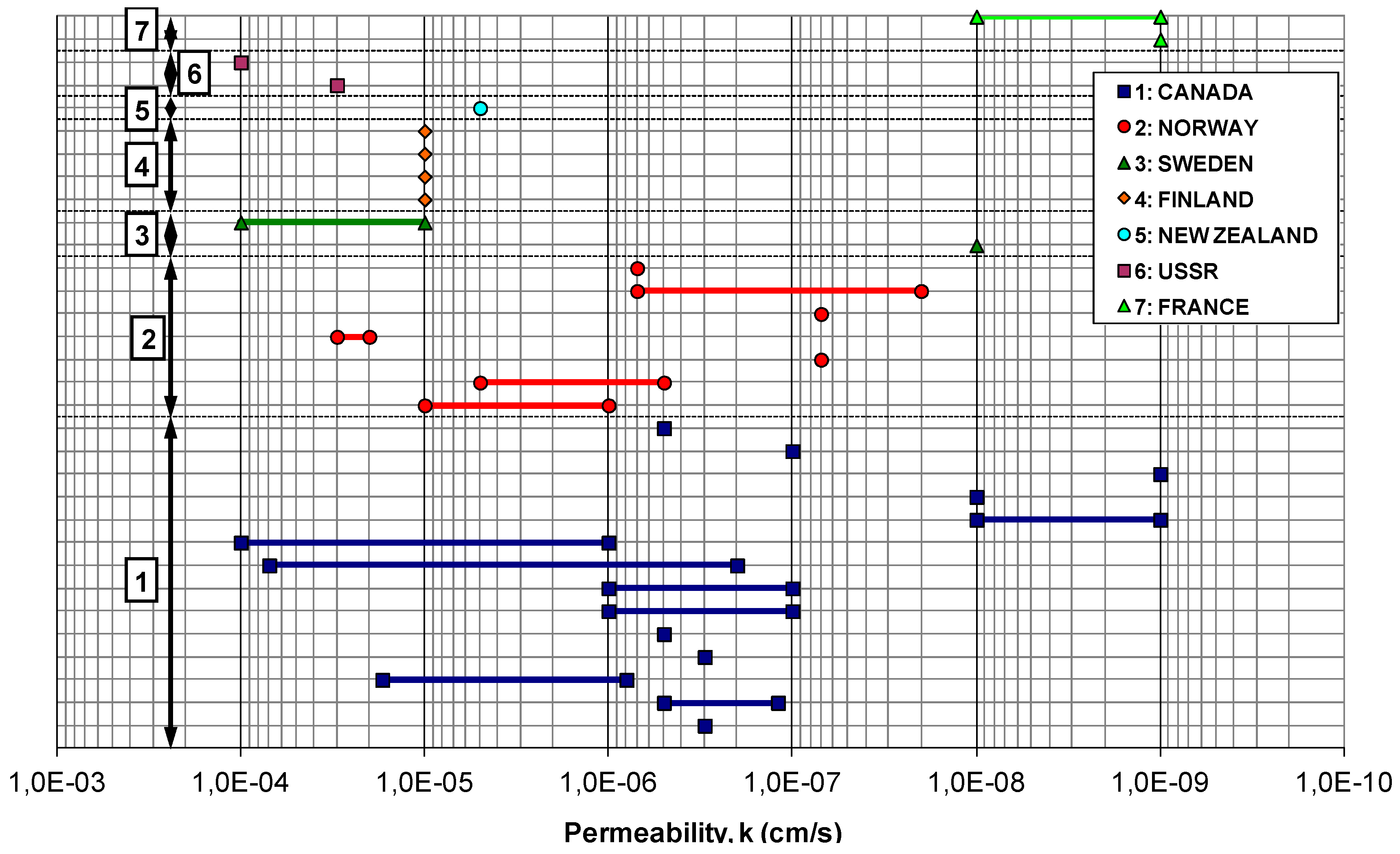
The permeability coefficient of the heterogeneous material varies within a wide range of values that will depend on the type of material and its granulometric distribution. To define the range of variability, experimentation on different materials is necessary. Figure 1, from data of [10], shows permeability coefficients of moraine materials that have been used for the construction of earth dams in Canada, Norway, Sweden, Finland, New Zealand, the former Soviet Union and France. In this figure, it can be seen that it is not possible to establish a mean value to determine the permeability values present in a moraine material, given that its range of variability is enormous. Analyzing the available permeability data, it can be indicated that these have a lot of dispersion, varying the permeability coefficient between maximum values of 10⁻³ cm/s and minimum values of 10⁻¹⁰ cm/s, with average value of the permeability coefficient around 10⁻⁵–10⁻⁶ cm/s.

Some dams that have been built with a heterogeneous core formed by moraine material are: LG2 Main Dam (Quebec, Canada), which is 160 m high and has a length of 2.9 km, Channel Dam (Russia), which is 68 m high, Presa Salve Faccha (Quito, Ecuador), which has a maximum height of 44 m and a coronation length of 190 m, and Slottmoberget Dam (Norway), which is 37 m high. In addition, there are also dams such as Uljua (Finland), which is 13 m high, made up of moraine material in a thin central core and which was also founded on a moraine deposit. There are also examples of other typologies where heterogeneous material is used; for example, the Finstertal Dam (Austria) has a maximum height of 95 m in the axis and was built with a 0.4H:1V inclined asphalt core, using glacial moraine material for the construction of part of the downstream shoulder.

Numerous studies of seepage through earth-fill dams have been conducted using physical models [11,12,13], because these give a general picture of the seepage behavior through earth-fill dams, including the phreatic line and the flow rate. As physical modeling has some limitations, numerical modeling, based on mathematical solutions, are used in many studies [14,15,16] to solve problems of seepage research. Al-Janabi et al. [17] investigated the seepage through earth-filled dams using physical, mathematical and numerical models, obtaining a good fit between them. This seepage analysis revealed that if a sufficient quantity of silty sand soil is available around the proposed dam location, a homogenous earth-fill dam with a medium drain length of 0.5 m thickness is a good design configuration. Zahedi and Aghajani [18] investigated the seepage behavior through the body of an earth-filled dam with different core shapes using a two-dimensional (2D) finite element seepage analysis. Choi [19] presented an evaluation of the seepage quantity of an earth dam using three-dimensional (3D) finite element analysis. In addition, Jamel [20] presented an investigation of the amount of seepage through a homogenous earth dam core by finite element software.

Despite progress, few studies have been conducted considering the statistical variability of core material properties. Some authors have achieved meritorious advances, analyzing different configurations of core zoning with low available permeabilities to optimize dam safety [21,22,23,24,25]. Thus, Kanchana and Prasanna [23] analyzed the use of various materials with different combinations to zone-type earth dams with a central impervious vertical core, and to study the behavior of the phreatic line at the downstream phase by varying the effective length of the horizontal drainage filter. Hassan Al [24] presented an application of finite element analysis to predict the two-dimensional steady-state water seepage through an earth dam with two soil zones resting on an impervious base. Continuing with this type of study, Fattah et al. [25] made a seepage analysis of a zoned earth dam by finite elements, studying the effect of several parameters, including the permeability of the embankment materials and the presence of an impervious core, together with its location and thickness. Special attention should be paid to the investigations of Mouyeaux et al. [26] and Guo et al. [27,28], who performed a probabilistic analysis of pore water pressures and stability of earth dams.

Some recent studies that show the need to control the core construction materials to avoid internal erosion phenomena are also worth mentioning. Khassaf [29] argued that seepage can cause weakening in the earth dam structure, followed by a sudden failure due to piping or sloughing, and presented a study to determine the quantity of seepage, exit gradient, hydraulic gradient and pressure head of zoned earth dams under the effect of changing core permeability and core thickness. Moreover, Hellström et al. [30] presented a study of fluid mechanics of internal erosion in embankment dams.

The present paper provides an analysis to evaluate the behavior of cored earth-filled dams using heterogeneous material in the context of seepage flow through the core and the gradients developed as a consequence of the flow of water, which indicates the behavior of the core against undesirable internal erosion problems that could occur. For this purpose, a Monte Carlo analysis is proposed, which allows assigning different permeability values in each of the core lifts, so that globally a certain distribution function is verified for the heterogeneous material.

Based on the statistical study carried out, some design charts for flow rates and maximum gradients for immediate use have been developed that allow judging whether a heterogeneous material can be used, in safety conditions, for the construction of the core of a dam. In this way, from the distribution of the permeability coefficient of the heterogeneous material to be studied (the mean value and its standard deviation), these charts could be used to know the failure probability of the dam in case this material under study is used for the dam core.

2. Theoretical Bases

The phenomenon of water seepage through a soil was established, under certain conditions, by the Laplace equation [31]. To undertake the study of seepage flow through the dam core, the following starting hypotheses were considered to be valid:

• Plain deformation. The 2D problem with water flow in the directions defined within the dam cross section was considered (Figure 2). Thus, the seepage flow per linear meter of the dam was studied and the total flow defined by the total length of the dam constructed. In Figure 2, the water level is represented at the top of the dam core, without freeboard.
• The seepage calculation was considered decoupled with the stress-strain analysis. Therefore, its compactness did not vary throughout the seepage process. The movement analysis is not specifically studied in this research.
• Darcy’s law was considered valid [32] and, therefore, the speed of the water flow in each point of the soil was proportional to the permeability of the soil and to the variation of the hydraulic potential with respect to its trajectory. It should be pointed out that due to the dam’s own construction process, which was carried out by compacted lifts of 20 to 40 cm thick. The permeability is not, in general, isotropic. Generally, the vertical direction follows the compaction direction of the lifts and has a considerably lower permeability than the horizontal direction.

From these hypotheses and considering the boundary conditions, the Laplace formula that solves the problem of seepage through to a dam is formulated in position coordinates (x, y) by:

$$k_x\frac{{\partial }^2\varphi }{\partial x^2}+k_z\frac{{\partial }^2\varphi }{\partial z^2}=0$$

(1)

where k_x and k_z are the permeabilities in the x and z direction, respectively, and ϕ is the hydraulic potential at each point on the ground. From this equation and its boundary conditions, its hydraulic potential and, therefore, its pore pressure, can be obtained at each point of the ground.

3. Finite Difference Method

Due to the assumed hypothesis of incompressibility during the seepage phenomenon, the flow modeling may be done independently of the usual mechanical calculation. Thus, (1), along with those that define its boundary conditions, are solved using a finite-difference approach. The study was carried out by developing computer numerical models, using a 2D analysis of a dam core with trapezoidal geometry. The calculations used to determine the water seepage flow rates were carried out using the commercial software of finite differences FLAC 2D (fast Lagrangian analysis of continua) [33], which was developed by the Itasca company (Minneapolis, Minnesota, USA). This program is widely used in the study of geotechnical problems.

The calculations were carried out using a simplified model of the dam (Figure 3), where only its core was modeled. This simplification was based on the starting hypothesis that the dam’s upstream and downstream shells are absolutely permeable and only the core is the impervious element of the dam, as generally the shoulders have a high permeability, or at least a higher permeability than the core (several orders of magnitude higher). Likewise, it was taken into consideration that the foundation of the core base is horizontal and behaves as an impervious element.

In every calculation, the mechanical boundary conditions (Figure 3) were set for level 0 (base of the core) and the foundation ground of the core was non-deformable (restriction of movement in the horizontal and vertical directions in all the nodes located at level 0), while for the rest of the nodes in the model, there were no imposed movement restrictions, which allowed them to move freely. It was also necessary to define the hydraulic boundary conditions (Figure 3), with the upstream face of the core being permeable and the water level located. As an additional hypothesis, it was also considered that the downstream face of the core was permeable and that, in addition, there was no tailwater level.

4. Study Methodology of Heterogeneous Material for the Dam Core

This section includes the calculation methodology of the numerical models that have been developed to carry out the analysis of seepage flows through the core of the dam and also of the maximum gradients produced in it, depending on the values of the coefficients of permeability that were adopted for the material that constitutes the core.

In each numerical model, the core of the dam has been discretized in a certain number of lifts. In order to know the behavior of a dam core built with heterogeneous materials, which is characterized by a large dispersion of permeabilities, the implemented calculation model allows assigning different permeability values for each of the lifts of the core with the condition that the permeability of the whole core is adjusted to a certain distribution function (previously defined).

4.1. Model of Dam Core Geometry

The dam core was assumed to be symmetrical, with inclinations of both upstream and downstream faces 1H:4V as shown in Figure 2 (usual value of the inclination for dam cores built with heterogeneous materials), and a core height of 50 m was considered. The top width of the core was established at 8 m and, therefore, the width of the base was 33 m.

Regarding the hydraulic boundary conditions, it was considered that the upstream face of the core was permeable and that the water level was located at elevation 50 (top of the core). It was also considered that the downstream face of the core was permeable and, in addition, there was no tailwater level. Likewise, it has been hypothesized that there is no seepage through the dam’s support substrate, but rather that seepage occurs only through the core of the dam.

Figure 2 shows the geometry that served as the basis for the elaboration of the calculation model that was prepared. The origin of coordinates (X = 0, Y = 0) was arbitrarily taken at the heel of the core for all the calculations that were carried out.

4.2. Calculation Phases of the Numerical Model

The construction of the core has been simulated by lifts. These zones have different permeabilities according to a lognormal distribution function and each zone is assigned a constant permeability but with a different value than another zone. Thus, the dimension of each zone of homogeneous permeability has been decided on a constructive criterion: (a) the lifts are generally compacted between 20–40 cm thick—to place three lifts per meter, a thickness of 33 cm has been chosen; (b) the length of the zone refers to the width covered by a compaction machine (machine that circulates perpendicular to the section of the dam), which is usually between 3–4 m wide—a zone length of 4 m has been chosen. In this way, the zones or lifts are 4 m × 0.33 m to represent material that is placed simultaneously, that is, with the same origin within the material storage for the construction of the core.

Each lift is, in general, 4 m wide (some are somewhat wider and others a little narrower, to adjust to the geometry of the core slopes) and 0.33 m thick (with three lifts per every meter of height of the dam core). Each lift is generally made up of four elements (which are made up of smaller elements; for example, some are made up of two elements, while others have a greater number of elements, namely up to six). The construction of the dam core has been simulated, therefore, in 150 stages, obviously starting from the base of the core and reaching the top of it (until completing the 50-m height of the core with a total of 768 lifts). In all calculations, it has been assumed that the placement of the material is carried out under saturated conditions.

The calculation phases have been the following:

• The first row of lifts is placed to constitute the base of the core and the mechanical boundary conditions are implemented, which only affect the lower nodes (Y = 0) of the elements of this first lift (rigid foundation, that is, constraint of horizontal and vertical displacements at the core base). Under these conditions, the first calculation of the construction stage has been carried out.
• Starting from the lower row of lifts of the core base, the simulation of the construction of the dam core was continued. For this, 149 more calculation stages have been carried out, until reaching the top of the dam core.
• Once the simulation of the construction of the dam core was finished, the simulation of the filling of the reservoir was carried out, placing the water level at a height of 50 m from the base of the core. For this, it was necessary to implement in the numerical model the hydraulic boundary conditions and the hydraulic properties of the materials that constitute the dam core (permeability coefficients fundamentally).

4.3. Seepage Path and Streamlines

For each distribution of permeabilities in the lifts of the dam core, the seepage flow through the core and the value of the maximum gradient occurred as a consequence of the circulating water was obtained. In normal practice, it is usually recommended that the seepage flow rates be limited below reference threshold values, usually set by the dam technicians.

The study of the gradient has the objective to show that the seepages running through the dam core do not produce internal erosion phenomena. References such as the dam project recommendations in Russia [34] indicate that the critical gradient may be around 5, which is why it is usual to recommend the construction of waterproof elements in dams with thicknesses greater than 20% of the water height. For this reason, in the calculations, the maximum gradient was determined by identifying the area of the core (lift, height within the core of the dam, etc.) where it should be placed, following the hypotheses of the current work. It was assumed that the gradient could determine the design of the core and could be the one that occurs in some of the lifts that form the downstream face of the core. Moreover, it could be evaluated according to what is indicated in the diagram and in the expression shown in Figure 4, where hp_i is the hydraulic potential in element “i,” d_1-i is the distance from the center of element 1 to the center of element “i” and grad(T_i) represents the value of the gradient in the lift “i.” Once the values of the 150 gradients (one for each of the 150 lifts located in the final 4 m of the downstream face of the dam core) were calculated, the maximum value of this gradient can be obtained, thus determining at what height of the dam core (in what lift) is produced.

4.4. Permeability Distribution

The material of the construction of the dam core is heterogeneous and, consequently, presents highly variable permeability values. Initially, tests have been done with various distribution functions, trying to choose a type of permeability distribution function that is easy to use and representative of a variable such as permeability (the normal distribution function, among others, was discarded because it provided negative values).

Due to its simplicity and because it responds to the characteristics of a physical variable such as permeability, the lognormal was chosen as the distribution function. The lognormal distribution function has two characteristic parameters: the arithmetic mean of the logarithm of the data and the standard deviation of the logarithm of the data, and it fits well to parameters that are themselves the product of numerous random quantities. Furthermore, the mathematical mean in the lognormal distribution is greater than its median. Therefore, it attaches greater importance to large values of failure rates than a normal distribution and is thus generally on the side of safety.

The distribution function that must be fulfilled for the set of the values of all the lifts is the condition that merges all the different values of each zone, and it is considered that this distribution function is the same as the heterogeneous natural soil of the site (in our case it has been considered a lognormal distribution function). However, the autocorrelation of the random field to describe a spatial correlation, which decreases with an increasing distance between two lifts, has not been considered.

Various lognormal distribution functions have been used, where their two characteristic parameters have been varied to cover a wide spectrum of possible permeabilities of the heterogeneous material. Based on the characterization of the permeability of heterogeneous materials referenced by some authors [6,7,8,9], four mean permeability values have been taken as representative of this type of heterogeneous materials: 10⁻⁵, 5 × 10⁻⁶, 10⁻⁶ and 5 × 10⁻⁷ cm/s. The value of the standard deviation of the distribution function has been chosen, indirectly, by fixing the dispersion of the permeability. To do this, we start from the known expressions of the mean value ${\mu }_x$ and standard deviation ${\sigma }_x$ of a variable x with lognormal distribution, based on the mean value ${\mu }_y$ and standard deviation ${\sigma }_y$ of the variable y = log x with normal distribution:

$${\mu }_x=e^{\left[{\mu }_y+\frac{{\sigma }_y^2}{2}\right]}$$

(2)

$${\sigma }_x^2=\left[e^{{\sigma }_y^2}-1\right]e^{\left[2{\mu }_y+{\sigma }_y^2\right]}$$

(3)

Therefore, using Equations (2) and (3), for a mean permeability ${\mu }_x=k_m$ and a variance ${\sigma }_x^2=v$ of the lognormal distribution of permeability, it is possible to obtain:

$${\mu }_y=\ln \frac{k_m}{\sqrt{1+\frac{v}{k_m^2}}}$$

(4)

$${\sigma }_y=\sqrt{\ln \left(1+\frac{v}{k_m^2}\right)}$$

(5)

That is, with different values of the variance of permeability v, different lognormal distribution functions are obtained, all of them with mean permeability $k_m$. These distribution functions will be more “open” or more “closed” depending on the value of the variance, v, adopted, and in order to be completely defined, it has been necessary to set extreme values Y_f (maximum value of permeability considered in the lognormal function) and Y_i (minimum value of permeability considered in the lognormal function) (Figure 5).

To fix the extreme values Y_f and Y_i of the lognormal distribution function, the concept of failure probability has been introduced. Brown [35] indicates that the probability of failure for dams is of the order of p = 10⁻⁴ to 10⁻⁵. Thus, one of the extremes of the distribution function (the maximum, Y_f) has been fixed, proceeding to calculate the minimum extreme, Y_i, imposing the condition that the lognormal distribution function between Y_f and Y_i contains a probability of (1−p), where p = 10⁻⁵ has been taken, as indicated above. The maximum extremes (Y_f) of the lognormal distribution function that have been chosen to carry out the calculations have been 5 × 10⁻³, 10⁻³, 5 × 10⁻⁴ and 10⁻⁴ cm/s. Thus, once these values of the maximum extremes of the distribution function have been fixed and imposed, the values of the minimum extremes (Y_i) have been calculated and collected in

Table 1. Minimum extreme values, Y_i, of the distribution functions used to carry out the different calculations.

Mean Permeability (cm/s)	Yf (cm/s)	Yi (cm/s)	Yf (cm/s)	Yi (cm/s)	Yf (cm/s)	Yi (cm/s)	Yf (cm/s)	Yi (cm/s)
10−5	5 × 10−3	9.15 × 10−10	10−3	2.30 × 10−8	5 × 10−4	7.40 × 10−8	10−4	7.30 × 10−7
5 × 10−6		8.10 × 10−11		3.20 × 10−9		1.16 × 10−8		1.44 × 10−7
10−6		6.15 × 10−14		1.61 × 10−11		9.15 × 10−11		2.32 × 10−9
5 × 10−7		5.75 × 10−16		1.04 × 10−12		8.09 × 10−12		3.20 × 10−10

with the condition of covering a probability equal to 99.999%. As can be seen, a wide spectrum of permeabilities has been covered, reaching very low minimum values (Y_i = 5.75 × 10⁻¹⁶ cm/s) in some cases.

4.5. Procedure to Assign Permeabilities to Each Lift of the Core

A programming code has been developed that, associated with the FLAC program, enables a random permeability to be assigned to each lift of the model in such a way that the set of permeabilities assigned to the 768 lifts that make up the core fit a lognormal distribution function. This procedure for assigning permeabilities to each lift, therefore, obtains different results each time the model calculation is carried out, because the different permeabilities (that jointly respond to a lognormal distribution law) are positioned in each model in different lifts. Therefore, the result of the calculations (flow or maximum gradient) turns out to be a random variable of some unknown probability distribution that must be investigated. In this regard, and as the number of possible combinations when assigning permeabilities to the lifts is undefined, a Monte Carlo analysis is carried out (with 1000 calculation models for each distribution considered) that allows studying the convergence and the distribution of the results of flows and maximum gradients obtained.

4.6. Analysis Cases

Considering the four mean permeability values indicated and the four permeability dispersion intervals considered from the above-mentioned minimum and maximum extremes, 16 distribution functions applicable to both isotropic and anisotropic cases are obtained.

Table 2. Analysis cases and number of calculations models.

Case	Permeability	Lognormal Distribution Characteristics			Number of Calculation
		kh,media (cm/s)	Yf (cm/s)	Yi (cm/s)
1	Isotropic (kh = kv)	10−5	5 × 10−3	9.15 × 10−10	1000
2			10−3	2.30 × 10−8	1000
3			5 × 10−4	7.40 × 10−8	1000
4			10−4	7.30 × 10−7	1000
5		5 × 10−6	5 × 10−3	8.10 × 10−11	1000
6			10−3	3.20 × 10−9	1000
7			5 × 10−4	1.16 × 10−8	1000
8			10−4	1.44 × 10−7	1000
9		10−6	5 × 10−3	6.15 × 10−14	1000
10			10−3	1.61 × 10−11	1000
11			5 × 10−4	9.15 × 10−11	1000
12			10−4	2.32 × 10−9	1000
13		5 × 10−7	5 × 10−3	5.75 × 10−16	1000
14			10−3	1.04 × 10−12	1000
15			5 × 10−4	8.09 × 10−12	1000
16			10−4	3.20 × 10−10	1000
17	Anisotropic (kh = 10 × kv)	10−5	5 × 10−3	9.15 × 10−10	1000
18			10−3	2.30 × 10−8	1000
19			5 × 10−4	7.40 × 10−8	1000
20			10−4	7.30 × 10−7	1000
21		5 × 10−6	5 × 10−3	8.10 × 10−11	1000
22			10−3	3.20 × 10−9	1000
23			5 × 10−4	1.16 × 10−8	1000
24			10−4	1.44 × 10−7	1000
25		10−6	5 × 10−3	6.15 × 10−14	10,000
26			10−3	1.61 × 10−11	1000
27			5 × 10−4	9.15 × 10−11	1000
28			10−4	2.32 × 10−9	1000
29		5 × 10−7	5 × 10−3	5.75 × 10−16	1000
30			10−3	1.04 × 10−12	1000
31			5 × 10−4	8.09 × 10−12	1000
32			10−4	3.20 × 10−10	1000

summarizes the characteristics of the 32 cases analyzed and the number of calculations that have been carried out, according to the Monte Carlo analysis, with each permeability distribution function. For each case of the Monte Carlo analysis, 1000 calculation models have been made, verifying the convergence of the results analyzed from the 200 to 300 calculation models. In case 25, the Monte Carlo study has been extended to 10,000 cases in order to see the validity of the analysis.

4.7. Results of Flow Rate and Maximum Gradient

In each of the 32 case studies, a Monte Carlo analysis has been carried out, obtaining the results of seepage flows and maximum gradients for each of the distribution functions. It is of great interest to represent the graphs that include the distribution of seepage flows through the core, the distribution of maximum gradients and the distribution of the height of the core where the gradients are greater. Thus, in Figure 6 these graphs have been represented for case 4 (which correspond to an isotropic permeability where the highest flow rate of all the distribution functions has been obtained) and in Figure that is presented shortly after Figure 7 below—Figure 8—these representations are shown for case 29 (which correspond to an anisotropic permeability where the largest gradient of all distribution functions has been obtained). A similar analysis was performed for the 32 calculation cases.

In case 4 (Figure 6), for the 1000 calculations carried out, a mean flow value of 0.551 L/min/m was obtained, with maximum and minimum values of 0.62 L/min/m and 0.495 L/min/m, respectively, and a standard deviation of 0.017 L/min/m. The value of the maximum gradient turned out to be variable between 3.0 and 1.94, with a mean value of 2.41 and standard deviation of 0.183. The highest values of the maximum gradient were obtained for flow values of the order of 0.55 L/min/m and for heights above the base of the dam core of less than 1 m.

The mean flow rates and mean maximum gradients for 20, 50, 100, 200, etc. calculations were also obtained, observing that, in general, for a number of calculations greater than 300, the mean value obtained from these two variables were similar to the one obtained when 1000 were calculations performed, as shown in Figure 7.

On the other hand, in case 29 (Figure 8), from the 1000 calculations that were made, a mean flow value of 0.00075 L/min/m was obtained, with maximum and minimum values of 0.0072 L/min/m and 0.0002 L/min/m, respectively, and a standard deviation of 0.035 L/h/m.

Although in most of the calculations that were carried out, the obtained flows were below 0.20 L/h/m, in eight calculations (0.8% of the total of the calculations carried out), flows were obtained above the indicated value. Specifically, the highest flow value was obtained for the calculation model n° 924 of 1000 (0.0072 L/min/m), as a consequence of the particular distribution of permeabilities in the core of the dam shown in the Figure 9; thus, in this calculation the highest permeability values, of the order of 10⁻⁴ cm/s, are located in several of the lifts of the core (located at about 41.5 m, 26.8 m, 22.5 m and 22 m high above the core base), as shown in Figure 9. In the rest of the lifts, the assigned permeability was within the range 3.8 × 10⁻¹⁴ to 4 × 10⁻⁵ cm/s.

In case 29, the mean maximum gradient that was obtained was of the order of 3.58, obtaining maximum and minimum values of 8.61 and 1.35, respectively, and a standard deviation of 1.29. The highest values of the maximum gradient were reached for flow values of the order of 0.00083 L/min/m, or even lower, and for heights above the base of the dam core below 10 m. For the values of the highest flow rates that were obtained in this calculation case (flows of the order of 0.0067–0.0075 L/min/m), the gradients obtained were low, something above 2.

Similarly, in case 29, for a number of calculations greater than 200–300, the mean value obtained from these two variables turned out to be substantially the same order as that obtained for the set of 1000 calculations performed.

Finally, it should be noted that the convergence analysis for the Monte Carlo simulation expanded to 10,000 calculation models of case 25 allowed the validation of the analyzes carried out in the rest of the cases, as a not very significant variation was obtained for the mean values of flow and maximum gradient between the first 1000 calculation models and the 10,000. In Figure 10, the convergence of the mean value and standard deviation of the maximum gradient are shown.

4.8. Adjustment of Flow and Maximum Gradient Distribution Functions

In the previous section, the distribution functions of the flow rates and the maximum gradients in calculation cases 4 and 29 have been graphically shown (and that were carried out in the same way for all calculation cases). From these representations, the adjustments of these distribution functions have been made, obtaining in this way, mathematical expressions from which it is possible to transform these discrete functions into other continuous ones, thus allowing a probabilistic handling of flows and maximum gradients. These distribution functions have been adjusted in this research by means of continuous functions of sigmoid type (continuous and differentiable function that allows a very handled probabilistic treatment as there are no singular points), according to the expression below:

$$N=\frac{A}{1+e^{B+CX}}$$

(6)

where N is the number of calculations, X is the variable that is calculated in each case (the seepage flow normalized by permeability, Q/k, or the maximum gradient, i), A is the number of Monte Carlo calculation models (A = 1000) and B and C are adjustment parameters obtained through the least squares method and that are presented for all cases in

Table 3. Statistical analysis of the adjustment parameters B and C for the flow and the maximum gradient distribution functions.

Case Study		Distribution Function			Adjustment Parameters
		kh,mean (cm/s)	Yf (cm/s)	Yi (cm/s)	Seepage Flow Rate		Hydraulic Gradient
					B	C	B	C
Isotropic permeability distribution	1	10−5	5 × 10−3	9.15 × 10−10	−12.24	4.33 × 10−4	−11.74	4.76
	2	10−5	10−3	2.30 × 10−8	−23.59	5.52 × 10−4	−13.80	5.90
	3	10−5	5 × 10−4	7.40 × 10−8	−30.30	6.36 × 10−4	−14.94	6.38
	4	10−5	10−4	7.30 × 10−7	−55.28	9.99 × 10−4	−22.41	9.22
	5	5 × 10−6	5 × 10−3	8.10 × 10−11	−8.38	3.77 × 10−4	−10.22	4.03
	6	5 × 10v6	10−3	3.20 × 10−9	−19.03	5.10 × 10−4	−12.97	5.42
	7	5 × 10−6	5 × 10−4	1.16 × 10−8	−23.91	5.49 × 10−4	−13.36	5.69
	8	5 × 10−6	10−4	1.44 × 10−7	−39.36	7.36 × 10−4	−18.12	7.62
	9	10−6	5 × 10−3	6.15 × 10−14	−3.02	2.72 × 10−4	−6.47	2.37
	10	10−6	10−3	1.61 × 10−11	−7.90	3.48 × 10−4	−10.18	4.05
	11	10−6	5 × 10−4	9.15 × 10−11	−11.39	4.02 × 10−4	−11.72	4.76
	12	10−6	10−4	2.32 × 10−9	−24.41	5.72 × 10−4	−13.71	5.84
	13	5 × 10−7	5 × 10−3	5.75 × 10−16	−2.36	3.81 × 10−4	−5.08	1.79
	14	5 × 10−7	10−3	1.04 × 10−12	−5.40	3.14 × 10−4	−8.29	3.21
	15	5 × 10−7	5 × 10−4	8.09 × 10−12	−8.27	3.69 × 10−4	−10.43	4.16
	16	5 × 10−7	10−4	3.20 × 10−10	−19.25	5.14 × 10−4	−12.41	5.15
Anisotropic permeability distribution	17	10−5	5 × 10−3	9.15 × 10−10	−19.18	1.29 × 10−3	−8.65	2.87
	18	10−5	10−3	2.30 × 10−8	−34.99	1.46 × 10−3	−11.65	4.54
	19	10−5	5 × 10−4	7.40 × 10−8	−41.00	1.52 × 10−3	−13.70	5.75
	20	10−5	10−4	7.30 × 10−7	−80.22	2.54 × 10−3	−21.60	10.37
	21	5 × 10−6	5 × 10−3	8.10 × 10−11	−14.05	1.29 × 10−3	−7.90	2.48
	22	5 × 10−6	10−3	3.20 × 10−9	−26.50	1.31 × 10−3	−10.27	3.74
	23	5 × 10−6	5 × 10−4	1.16 × 10−8	−30.94	1.29 × 10−3	−11.85	4.66
	24	5 × 10−6	10−4	1.44 × 10−7	−58.83	1.95 × 10−3	−17.42	7.91
	25	10−6	5 × 10−3	6.15 × 10−14	−5.32	1.60 × 10−3	−5.33	1.52
	26	10−6	10−3	1.61 × 10−11	−14.25	1.30 × 10−3	−7.75	2.39
	27	10−6	5 × 10−4	9.15 × 10−11	−19.84	1.33 × 10−3	−9.25	3.04
	28	10−6	10−4	2.32 × 10−9	−32.96	1.37 × 10−3	−12.43	4.92
	29	5 × 10−7	5 × 10−3	5.75 × 10−16	−3.66	2.64 × 10−3	−4.62	1.31
	30	5 × 10−7	10−3	1.04 × 10−12	−9.90	1.39 × 10−3	−6.75	1.99
	31	5 × 10−7	5 × 10−4	8.09 × 10−12	−14.19	1.32 × 10−3	−7.76	2.44
	32	5 × 10−7	10−4	3.20 × 10−10	−25.43	1.26 × 10−3	−10.36	3.76

.

4.9. Discussion of Results

This section collects jointly the results obtained in the 16,000 calculations that were made considering the distribution of isotropic permeability in the core of the dam and the other 25,000 for the case of anisotropic permeability. First, the results of the isotropic calculation cases 1 to 16 have been grouped in order to know, in a global way, the records that were obtained. This is a highly variable set of calculations, which were performed taking four different horizontal mean permeabilities (10⁻⁵, 5 × 10⁻⁶, 10⁻⁶ and 5 × 10⁻⁷ cm/s) and 16 different permeability distribution functions, with very wide ranges of variation (Y_f = 5 × 10⁻³ to 10⁻⁴ cm/s; Y_i = 7.30 × 10⁻⁷ to 5.75 × 10⁻¹⁶ cm/s). Summary graphs of flow rates and maximum gradients obtained in this group of 16,000 calculations with isotropic permeability are shown in Figure 11.

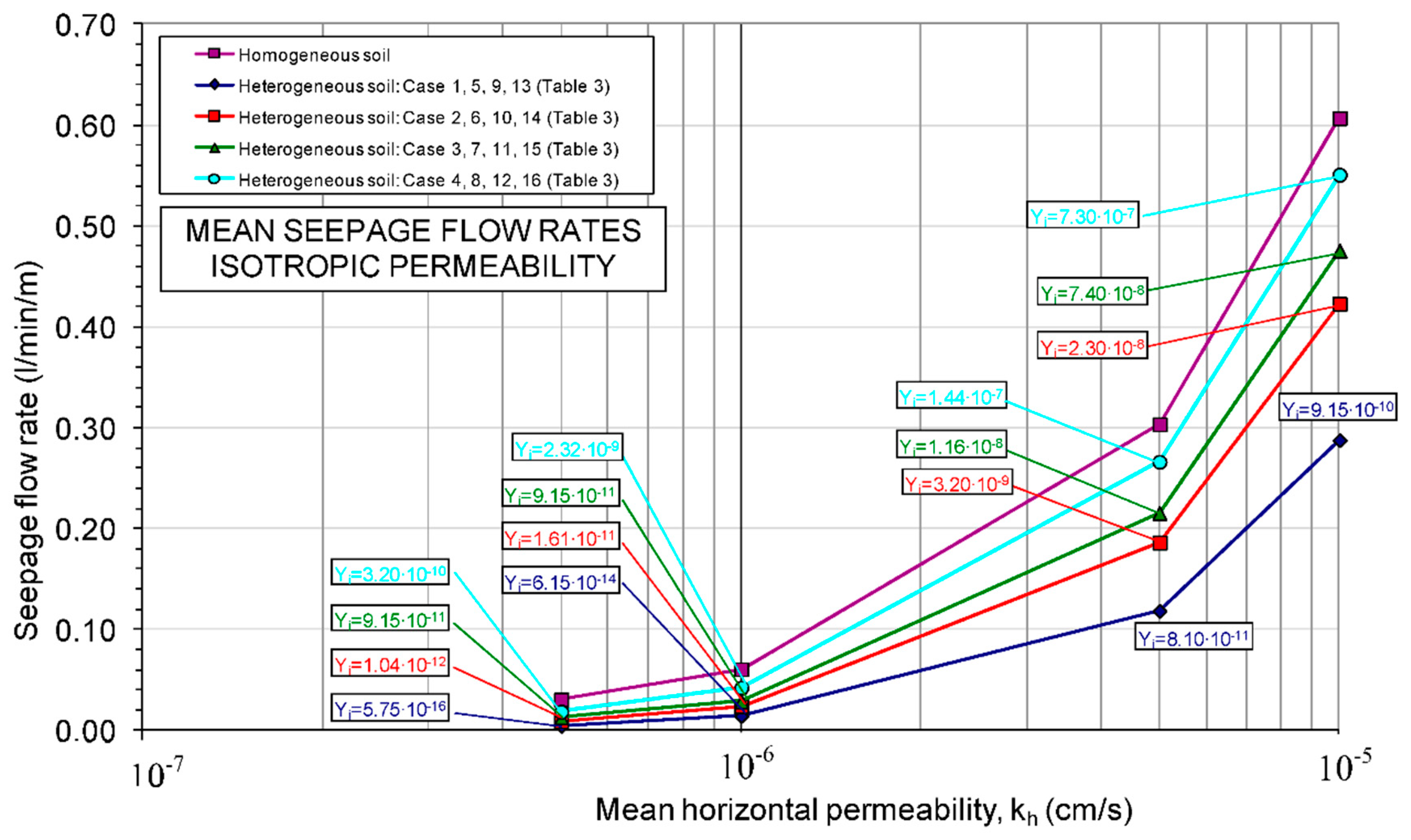
In Figure 12 the mean flow values for each of the isotropic permeability distribution functions that were used to carry out these calculations have been represented, as well as in the case of using a homogeneous value of the permeability equal to the mean value. As can be seen, the mean flow values were highly variable, within the range of 0.02 L/min/m to 0.54 L/min/m. Higher flow rates were obtained as the mean permeability value increased, for more “closed” ranges of the permeability distribution function (a smaller “distance” between Y_f and Y_i) and also for distribution functions with a higher Y_i (lower probability that the distribution function contains very low permeabilities).

Regarding the maximum gradients, a certain distribution of the results obtained around a mean value was observed for the 16 cases of isotropic permeability treated together. This mean value of the maximum gradient turned out to be of the order of 2.49, with a maximum value of 8.56 and a minimum value of 1.53, with a standard deviation of 0.50. On Figure 11, the adjustment for the distribution function of the maximum gradient of this group of 16,000 calculations was made, where the constants of best adjustment for the sigmoid curve (6) are A = 16,000, B = 4.484 and C = −10.982.

Thus, in the cases of isotropic permeability, the highest values of the maximum gradient (i > 6) were obtained for flow values below 0.01 L/min/m and for heights above the base of the dam core lower than 17 m. In the calculations in which the highest flow values were recorded (Q > 0.70 L/min/m), however, the values of the maximum gradients obtained were low, in the range 1.65 to 2.45. The mean values of the maximum gradients that resulted in these calculation cases from 1 to 16 were also analyzed. As a result of this analysis, Figure 13 was elaborated. As can be seen, the mean value of the maximum gradient turned out to be 2.49, and variable within the range 2.33 to 2.94. The highest mean values of the maximum gradients were obtained for those more “open” permeability distributions, for those calculations that were carried out taking a lower end (Y_i) of the range of variation of the lowest permeabilities, and for the calculations that they were made using a lower mean permeability value.

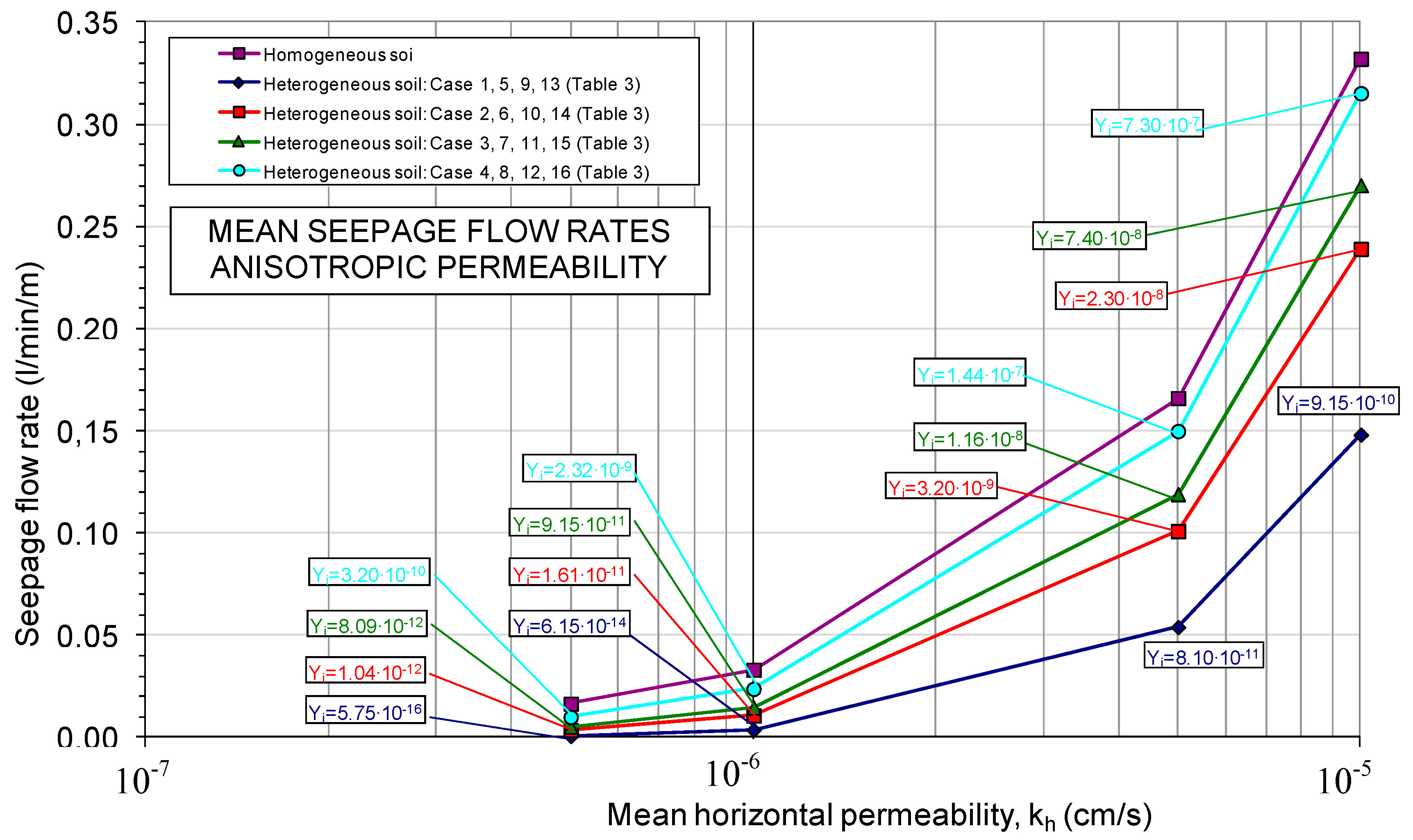
In the same way, the analysis of the 16 anisotropic cases has been carried out. Thus, in Figure 14 the summary graphs of flow rates and maximum gradients of the 25,000 calculations with anisotropic permeability have been presented.

Figure 15 has been prepared in which the mean values of the flow rates for each one of the anisotropic permeability distribution functions that were used to carry out these calculations have been represented. The mean values of the flow rates were also highly variable, within the range of values from 0.015 L/min/m to 0.31 L/min/m. In the same way as in the calculations made with isotropic permeability distribution, higher flow rates were obtained as the mean value of horizontal permeability increased, as well as for more “closed” ranges of the permeability distribution function and for distribution with a higher Y_i.

In relation to the maximum gradients, the analysis of the anisotropic cases also showed a distribution of the results obtained around a mean value. This mean value of the maximum gradient turned out to be of the order of 3.12, with a maximum value of 9.53 and a minimum value of 1.32, with a standard deviation of 1. The distribution function of the maximum gradient is adjusted in Figure 14, obtaining the sigmoid curve of best fit (6) corresponding to: A = 25,000, B = 1.853 and C = −5.633. Thus, for all anisotropic calculation models, the highest values of the maximum gradient (i > 8) were obtained for flow values below 0.01 L/min/m (with some slightly higher point values, around 0.05 L/min/m) and for heights above the base of the dam core lower than 13.5 m. In the calculations in which the highest flow values were recorded (Q > 0.30 L/min/m), however, the values of the maximum gradients obtained were low, in the range of 1.7 to 3.4. The mean values of the maximum gradients that resulted in these calculation cases 17 to 32 carried out were also analyzed. From this analysis, Figure 16 was obtained.

As can be seen, the mean value of the maximum gradient was of the order of 2.88, and variable within the range of 2.07 to 3.58. The highest mean values of the maximum gradients were obtained for those more “open” permeability distributions, for those calculations that were made taking the lower end (Y_i) of the range of variation of the lowest permeabilities, and for the calculations using a lower mean horizontal permeability value. In short, the behavior was similar to that observed for the calculations that were carried out with isotropic permeability distribution, although, in these other calculations carried out with anisotropic permeability distribution, in general, the mean values of the maximum gradients obtained were more elevated.

Based on the results shown for the 32 cases studied for both isotropic and anisotropic permeability, the following statements regarding the flow study can be concluded:

-

For the same mean value of horizontal permeability, the flow rates through the core are always higher in the calculations made considering the homogeneous core permeability than in the calculations that were made considering the permeability of the core as heterogeneous (Figure 12 and Figure 15).

-

The calculations carried out with anisotropic permeability, for which it has been established that the mean horizontal permeability is 10 times greater than the mean vertical permeability, provide lower flow values through the dam core compared to when the same calculations (same mean horizontal permeability and same range of variation of permeabilities) are carried out for isotropic permeability. In the calculations carried out considering the homogeneous permeability, lower flow rates were observed when anisotropic permeability distribution was considered in the dam core than when isotropic permeability distribution was considered.

-

For similar ranges of variation of the permeabilities (Y_i to Y_f), a lower value of the mean horizontal permeability implies lower values of the flow rates obtained.

-

Both with isotropic and anisotropic permeability distribution, for the same value of the upper end Y_f of the range of variation of permeabilities of the distribution function, the minimum, average and maximum flow rates increase as the value considered Y_i of the range of the permeability interval grows.

-

Similarly, as the lower value of the distribution function, Y_i, increases, the flow values also increase (even though the upper values of the distribution function, Y_f, decrease).

-

For the same horizontal mean permeability, the flow rate of the calculations is greater as the range of variation of the permeabilities (Y_i to Y_f) selected to carry out the calculations is more “closed.” Furthermore, in these cases in which the range of variation of the permeability coefficient is more “closed,” the variation between the maximum and minimum flows is also more “closed,” that is, the range of variation of the flows is more limited, obtaining the highest values of the minimum flows and the lowest values of the maximum flows.

For its part, regarding the study of maximum gradients, for all Monte Carlo cases, it can be concluded that:

-

The values of the maximum gradient, in general, are increased in the cases analyzed with anisotropic permeability compared to the calculations performed with isotropic permeability.

-

The range of variation of the mean values of the gradients has been less in the calculations carried out with isotropic permeability than in the calculations carried out with anisotropic permeability.

-

In any case, the mean values of the gradients have little variation in the different calculations that have been prepared. However, if the values of the maximum gradients are taken into account, the highest values obtained in each of the 32 cases decrease significantly when the calculations are made by taking the values lowest variation of the permeability range.

-

It has also been observed that with the decrease in the permeability values, the highest values of the maximum gradients increase, although the mean and minimum values of the maximum gradients hardly vary.

-

The permeability interval (Y_i to Y_f) considered to carry out the calculation has a clear influence on the value of the maximum gradient obtained: as the calculations are made with a more “closed” range of permeabilities, the values of the gradient obtained are more homogeneous, all of them closer to the mean value of the gradient corresponding to the calculation case.

-

The highest gradients that have been obtained are not necessarily associated with the highest flow rates. High gradients have been obtained for situations in which the flow rates through the dam core have been moderate and low, and similarly, low gradients were obtained for calculations with high values of the flow through the dam core (Figure 17).

-

In general, the highest gradients have been obtained for the lowest lifts of the dam core (near the foundation, for heights below 1–2 m) for the analyzed calculation situation: a study of gradients in the area of the downstream face of the dam core, where these will presumably be more determining factors (internal erosion problems, suffusion, remontant erosion, etc.) than in other areas of the dam core.

5. Design Charts

5.1. Object of the Charts

The calculations made with the Monte Carlo analysis have allowed to obtain mathematical expressions for the distribution functions of the flow rates through the core and of the maximum gradients produced in it, when this core is built using heterogeneous materials, which are characterized by different permeability distribution functions (log-normal in the study that was carried out). From the results obtained, it has been possible to elaborate a series of charts for the design of earth dams, in which the construction of these cores was simulated using heterogeneous materials. The proposed charts are suitable for the dams with similar configuration to the studied one, and new charts are necessary for significantly different cases.

The ultimate goal pursued with the elaboration of these charts is an engineering tool that allows the decision of if the dam built with a heterogeneous material in its core is safe, for certain admissible maximum values of the flows and gradients called “critical.” In this sense, critical flow is understood as that which cannot be exceeded as a consequence, for example, of hydraulic conditions in the basin, because this is established in the dam’s operating manual, and the critical gradient is that which would cause internal erosion problems in the core of the dam. Consequently, once these values of the critical flow rates and of the critical gradients are known, which must be initially set, and making use of these design charts that have been prepared, it will be possible to have elements of judgment that will allow to know, based on a simple geotechnical characterization of the heterogeneous material available, if it is valid to be used in the construction of the waterproof element of the dam.

5.2. Representation Criteria of the Charts

When a heterogeneous material is used for the construction of dam cores, it will generally not be possible to characterize it by means of a single value of permeability. Thus, as indicated, various calculations were carried out according to a Monte Carlo methodology, to know the flow network in the core of the dam when the permeability coefficients of the material were distributed as according to a distribution function, which was assumed to be log-normal.

Sixteen different log-normal functions were used to perform these calculations, varying the characteristic parameters that define them (Table 1 and Table 2): the mean value of the permeability coefficient (k_mean) and the extreme values between which the permeability coefficient can vary in each of the distribution functions (upper end: Y_f; lower end: Y_i), that is, the dispersion presented by the permeability distribution function.

In this way, the values of the variance (σ²) and the standard deviation (σ) of each of the distribution functions were defined and, therefore, the coefficient of variation could be known (CoV = σ/k_mean) of the permeability for each of these functions. This statistical parameter is dimensionless, which makes it possible to compare different sets of permeabilities (with different mean values and different dispersions). In Figure 18 below, the values of the coefficient of variation (CoV) that were estimated for each of the permeability distribution functions in relation to the values of the horizontal mean permeability (k_h,mean) are shown.

These values of the coefficient of variation relative to each one of the permeability distribution functions are represented on the abscissa axis of the design charts of the dam core built with heterogeneous materials. On the other hand, the ordinate axis will represent the probability of occurrence that would occur depending on the characteristics of the material that has been used for the construction of the core of the earth dam. In this way, a tool is available to quantify the level of risk that is assumed when using heterogeneous materials or in the execution of the waterproof element (a greater probability of occurrence of these design charts indicates a greater risk in the construction of the core of the dam).

5.3. Probability of Occurrence

As explained in a previous section, from the results of the calculations, the distribution functions of the flows and the maximum gradients in the core of the dam could be obtained. Sixteen distribution functions of flow rates and maximum gradients were obtained for the calculations that were carried out, considering the distribution of the isotropic permeability in the dam core, and another 16 for the calculations that were carried out adopting an anisotropic permeability distribution. All these distribution functions were adjusted by means of Equation (6), of which the adjustment coefficients are shown in Table 3.

The probability in a certain range of the variable of the flow or of the maximum corresponds to the area under the respective density function of each of these variables in that interval and, therefore, can be obtained from the distribution functions that were estimated, as shown graphically in Figure 19.

Despite the consistency of the proposed method, it is also advisable to indicate the main limitations to assess the probability of failure:

-

The main parameter that defines the seepage problem is permeability. Its value is one of the most difficult to determine with precision within the geotechnical field of dams. Taking into account a heterogeneous distribution with a wide range of permeability variability, it is not easy to choose the permeability estimators, and it is necessary to assume a distribution function that adequately fulfills the set of permeability values of the material.

-

A Monte Carlo analysis was performed, limited to a reasonable number of calculation cases that do not cover the tails of the distribution (with 1000 or 10,000 calculations it is not possible to cover probabilities of 10⁻⁴ or 10⁻⁵); therefore it was necessary to adjust the distribution functions to the flow rates and gradients obtained in order to be managed statistically.

5.4. Design Charts for Seepage Flow Rates through the Core

It is usual for the dam’s operating manual to include limitations that the flows must meet, which are usually values set according to the hydrology of the place (values of the seepage flows that, if exceeded, would be difficult to accept for the hydraulic management of the river) or from previous experiences in other dams in the area, etc. Therefore, these would be the aspects from which a value of the critical flow could be set.

The calculations of the water flow through the dam core made up of a single material (homogeneous and with a unique permeability coefficient for the entire set of material that constitutes the core) can be used as a reference. In this case, it was obtained that: (a) the calculations carried out with isotropic permeability distribution (k = k_h= k_v) resulted in a seepage flow rate through the core of (Figure 12): (Q/k)_hom = 101.20 m²/m; (b) the calculations carried out with anisotropic permeability distribution (k = k_h = 10 × k_v) resulted in a seepage flow rate through the core of (Figure 15): (Q/k)_hom = 55.35 m²/m.

In this way, the elaborated design charts have been represented for a “critical” value of the flow rate that has been defined in this research according to the following expression:

$${\left(\frac{Q}{k}\right)}_{crit}=\alpha {\left(\frac{Q}{k}\right)}_{hom}$$

(7)

where α = 1, 2/3, 1/2, 2/5, 1/3 has been taken (10 charts in total, five for the distribution of isotropic permeability and another five for the distribution of anisotropic permeability).

Therefore, on the ordinate axis of these design charts the probability was represented of exceeding a flow value α times less than the seepage flow through the core obtained in the calculations made considering homogeneous material, which has been called the probability of occurrence.

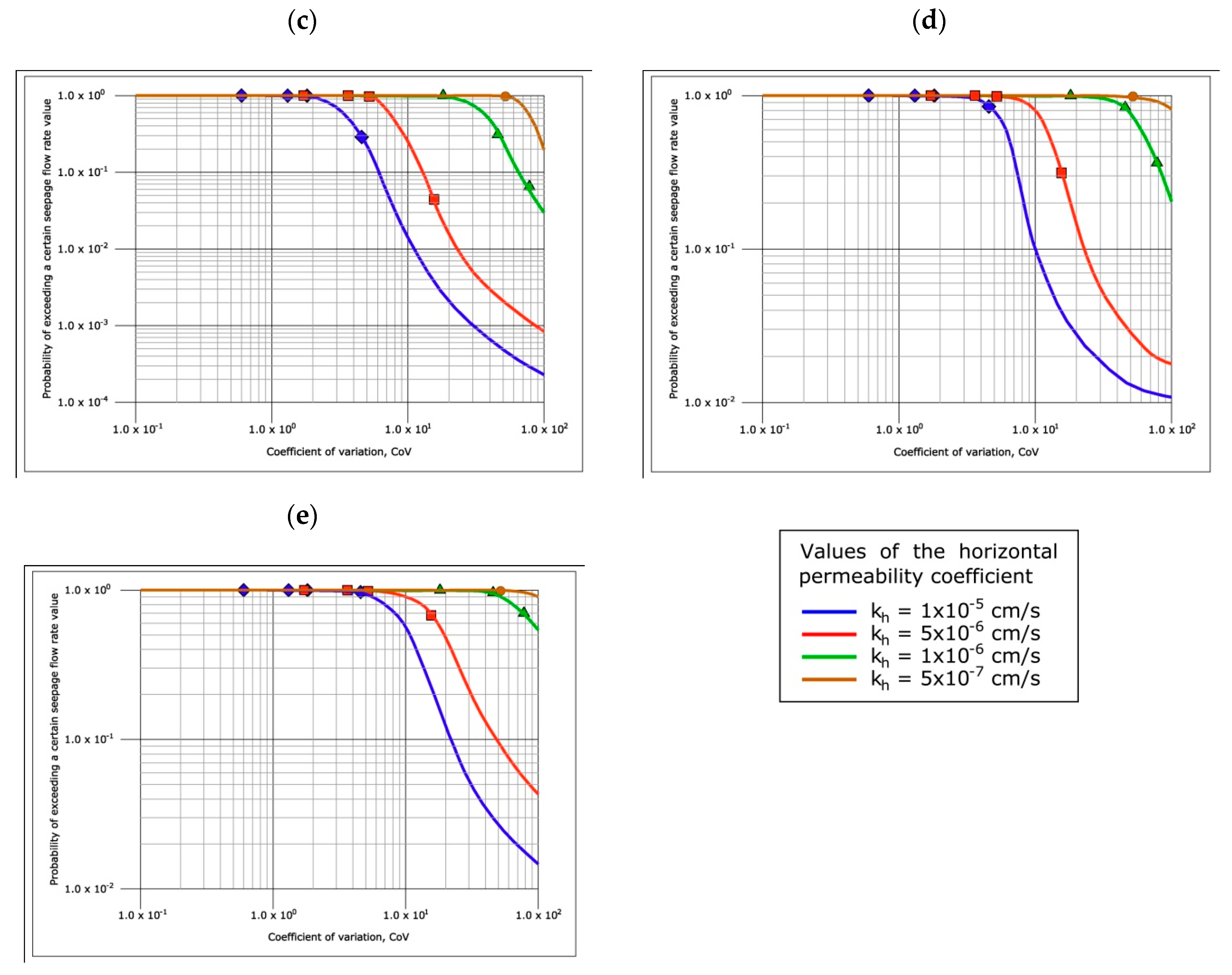
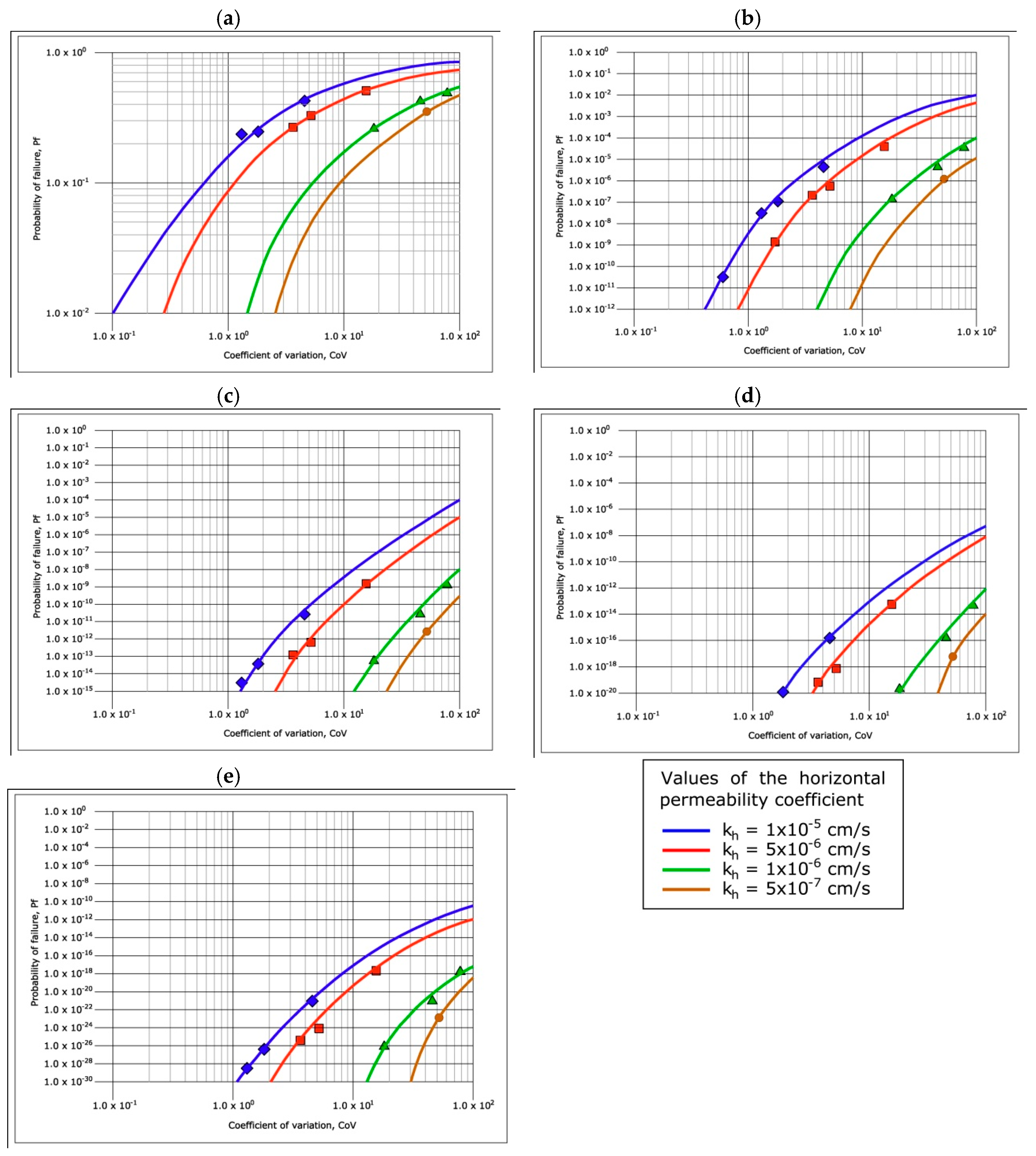
Figure 20 and Figure 21 include the design charts for seepage flows through dam cores made with heterogeneous materials where, as mentioned, the coefficient of variation corresponding to the distribution function of the permeability coefficients is shown on the abscissa axis and, on the ordinate axis, the probability of exceeding a certain value of the flow (probability of occurrence). These design charts have been prepared for the different values of α, so that in Figure 20 the charts corresponding to isotropic permeability distributions have been collected, while in Figure 21 the charts with the anisotropic permeability have been shown. Each of the points corresponding to the 32 Monte Carlo analysis performed according to the 16 isotropic distribution functions, and another 16 anisotropic have been marked on the charts. For the charts of Figure 20 and Figure 21, expression (6) has been used, and each equation in Table 3 corresponds to a CoV; therefore, each curve in each chart has four points plus the boundary conditions (P_r = 1 for CoV = 0, and P_r = 0 for unbounded CoV values). The best fit curve has been adjusted using sigmoid type functions that allow obtaining, for all curves, a coefficient of determination R² > 0.89. There are curves where the four points are not visible because some points are outside the range represented using sigmoid type functions that allow obtaining, for all curves, a coefficient of determination R² > 0.89.

The design charts for the flow rates show that a higher value of the coefficient of variation of the distribution function of permeability coefficients implies lower flow values for the core of the dam. The coefficient of variation will be the greater as the value of the standard deviation of the distribution rises. In the study carried out, the ranges of variation of the coefficient of variation were obtained by fixing one of the extremes of the permeability distribution function (the one with the highest permeability value, Y_f) and obtaining the other, the one that marks the value of the lowest permeability, Y_i, such that this distribution function of permeability coefficients between Y_f and Y_i contains a probability of (1−p), where p = 10⁻⁵.

Consequently, for very dispersed permeability distribution functions, with very high standard deviations (or, which is the same, with high coefficients of variation), very low values of Y_i were obtained, that is, many lifts of the dam have a high probability of being built with materials with low permeability coefficients and, therefore, the seepage flow through the dam core will be lower for those cases in which the coefficient of variation is high.

5.5. Design Charts for Maximum Gradients Recorded in the Core

The flow of water that circulates through the dam core produces a gradient that must be controlled to avoid internal erosion phenomena that could trigger pathologies. This analysis of the maximum gradients originated in the waterproof element of the dam is of even greater interest in the present case under study, where the possibility of using heterogeneous materials for the execution of the dam core is being analyzed and, therefore, where the maximum gradients that occur can become considerably higher than in a situation in which homogeneous materials with good characteristics are used.

Various design charts have been prepared based on various values of the critical gradient. To do this, the values of the maximum gradients obtained in the calculations of homogeneous material with a numerical model have been taken as initial reference. For this situation, it was obtained that: (a) in the calculations carried out with isotropic permeability distribution (k_h = k_v) the maximum gradient was: i_max = 2.526; (b) in the calculations carried out with anisotropic permeability distribution (k_h = 10 × k_v) the maximum gradient was: i_max = 1.937.

In this way, various design charts have been elaborated adopting critical values of the gradient according to the following expression incorporated in this research:

$$i_{crit}=\beta i_{max,hom}$$

(8)

where β = 1, 2, 3, 4 and 5 were used (10 charts in total, five for distribution of isotropic permeability and another five for distribution of anisotropic permeability).

Consequently, on the ordinate axis of these design charts, the failure probability that would occur for different values of the critical gradient presented by the heterogeneous material that is intended to be used in the construction of the dam core has been represented.

These values of the critical gradient of the material can be estimated by means of specific tests: HET (hole erosion test), SET (slot erosion test), JET (submerged jet erosion test), etc. In any case,

Table 4. Mean values of the critical hydraulic gradient [36].

Soil	Apron	Diaphragm/Core	Dam Body
Clay, clay concrete	15	12	8–2
Sandy clay	10	8	4–1.5
Clayey sand	3	2	2–1
Medium sand	-	-	1
Fine sand	-	-	0.75

has reproduced some values for the critical gradient that are included in [36], where it turns out that for the core element, the critical gradient could be variable between 2 and 12, approximately.

The design charts for the maximum gradients produced in the dam core executed with heterogeneous materials have been presented in Figure 22 and Figure 23, where the coefficient of variation corresponding to the distribution function of the permeability coefficients is presented on the abscissa axis, and the failure probability that would occur depending on the values of the maximum gradient produced and the critical gradient of the heterogeneous material used for the construction of the core on the ordinate axis. These design charts have been made for various values of β, so that Figure 22 shows the design charts relative to the isotropic permeability distributions, while Figure 23 shows the design charts corresponding to the anisotropic permeability distributions. Each of the points corresponding to the 32 Monte Carlo analyses carried out according to the 16 isotropic distribution functions and the 16 anisotropic distribution function have been marked on the chart. For the charts of Figure 22 and Figure 23, expression (6) has been used and each equation in Table 3 corresponds to a CoV; therefore, each curve in each chart has four points plus the boundary conditions (P_r = 0 for CoV = 0, and P_r = 1 for unbounded CoV values), so the best fit curve has been adjusted using sigmoid type functions that allow obtaining, for all curves, a coefficient of determination R² > 0.92. There are curves where the four points are not visible because some points are outside the range represented.

Based on the design charts for the maximum gradients produced, the following has been observed:

• The higher mean values of the permeability coefficient of the material used for the construction of the core corresponding to the greater failure probability.
• The higher values of the coefficient of variation of the distribution of the permeability coefficient of the material used for the execution of the core corresponding to a greater failure probability.
• The lower values of β used to make the design charts corresponding to a greater failure probability.
• The failure probabilities have been found to be greater when a material with an anisotropic permeability is used for the construction of the core.

5.6. Application Example

This section contains an example of the application and use of the design charts for dam cores made with heterogeneous materials that have been included in the previous section. The various stages that will have to be followed for the use of these charts will be the following:

• Carry out tests to determine the geotechnical characteristics of the available heterogeneous material: (a) identification tests: granulometry and plasticity; (b) state tests: dry density and natural humidity; (c) tests to determine the permeability of the material: it is recommended to carry out tests both in the field and in the laboratory, identifying the mean value of the permeability coefficient, the standard deviation and the coefficient of variation of the distribution of permeability coefficients obtained. In addition, it must be known whether the material behaves in an isotropic or anisotropic way, from the point of view of the permeability coefficient. Let us assume as a starting hypothesis, for this application example, that, after all these tests are carried out, it was obtained that the mean value of the horizontal permeability coefficient is k_h,mean = 10⁻⁶ cm/s, that the coefficient of variation of the distribution of the permeability coefficient is 10 and that the material shows anisotropic behavior from the permeability point of view, with k_h = 10 × k_v.
• Carry out tests to know the critical gradient of the heterogeneous material. For this purpose, for example, laboratory tests such as HET, SET, JET, etc. could be carried out, through which we can obtain the values of the critical gradient, i_crit, and, therefore, the value of β of the chart to use. As a hypothesis for this application example, it will be assumed that a critical gradient value was obtained equal to β = 2.
• Once it is known that the permeability distribution is anisotropic, and that the value of β is equal to 2, it will be possible to know which of the charts to use to guarantee certain reliability conditions with respect to the hydraulic gradient. In this case, the design chart to be used would be that of Figure 23b. Entering the abscissa axis of this design chart with a value of the coefficient of variation, CoV, equal to 10, the curve corresponding to the mean value of permeability of 10⁻⁶ cm/s would be chosen. By tracing a horizontal line on the ordinate axis, it would be obtained that, when constructing the dam core with a heterogeneous material of the characteristics indicated, the failure probability would be of the order of 10⁻⁵ (slightly lower), as has shown in Figure 24a.
• In relation to the flow, it would be necessary to know the condition that should be verified (a control flow could be set that would be expected to be exceeded with some probability for the conditions of heterogeneous material used in the construction of the core). In principle, in the absence of references in relation to this aspect on seepage flow rates, the maximum value of this flow rate through the core that should be admitted should be the one corresponding to the value of α = 1, which would correspond to the value of the flow rate through a dam core that has been executed with a single material, of homogeneous permeability.

In any case, if, for example, as a consequence of the hydric characteristics of the river bed downstream of the dam, or of any other recommendation that could be included in the dam’s operating manual in relation to the values of the seepage flows, the possibility of exceeding a certain value of the seepage flow through the dam core is limited, for example, of a half value (α = 0.50), the design chart of Figure 21c would have to be used.

Entering this design chart with a value of CoV = 10, and working with the permeability curve k_mean = 10⁻⁶ cm/s, the probability of exceeding a seepage flow rate through the core would be 0.50 times than it would be if the material were homogeneous, with p = 1, as shown in Figure 24b (as per the data, it can be indicated that, for the situation corresponding to α = 1, the probability of exceeding a seepage flow through the core is the same order as what would be obtained if the material with which this core had been built were homogeneous, slightly below 10⁻³ cm/s; see design chart Figure 21a).

The final conclusion for this assumption that has been raised as an example of the application and use of design charts is, therefore, that with this heterogeneous material whose characteristics were defined, the failure probability obtained is of the order of 10⁻⁵ (slightly below), that is, of the same order that is usually required (10⁻⁴ to 10⁻⁵, Brown [35]), although the required seepage flow rate will be exceeded in the dam core.

6. Conclusions

To control the seepage, geotechnical recommendations prescribe a high proportion of fines and a high homogeneity of geomechanical characteristics for the material used in the dam core. However, the volumes of soil required for the construction of an earth dam are usually of importance and the use of materials in the vicinity of the dam is often complicated because the existence of good quality materials with homogeneous properties is scarce in sites near the dam. Unfortunately, using and transporting soil with good geotechnical characteristics to construct the core in a faraway location is economically and environmentally unsustainable. Therefore, the possibility of using less suitable materials at the dam site as part of the core must be studied.

In this research, a study of heterogeneous materials for dam core, characterized by a wide range of permeability variation, has been carried out. Thus, the contrast of permeabilities between different lifts can produce uncontrolled seepage flows through the dam and high hydraulic gradients that must be restricted to avoid problems of internal erosion in the dam. Permeability values of the heterogeneous material have been assigned to each lift of the dam core, so that the set of all assigned permeabilities have a simplified random field with a lognormal distribution function. As there are an unaffordable number of ways to assign these permeabilities, a Monte Carlo analysis has been carried out, which has proven to be a very powerful tool to study the viability of heterogeneous material. Based on the results of the Monte Carlo analysis and using a basic geotechnical characterization, some design charts to know the failure probability of the dam in the event that this material was used in the dam core have been developed: a first group related to the seepage flows through the core of the dam and a second in relation to the maximum gradients that could be produced in the core of the dam.