Volatility Connectedness between Clean Energy Firms and Crude Oil in the COVID-19 Era


Abstract
1. Introduction
2. Related Studies
3. Data
4. Empirical Approach
4.1. Volatility Dynamic Connectedness
4.2. Dynamic Conditional Correlations
5. Empirical Results
5.1. Volatility Connectedness Analysis
5.2. Correlation and Portfolio Management
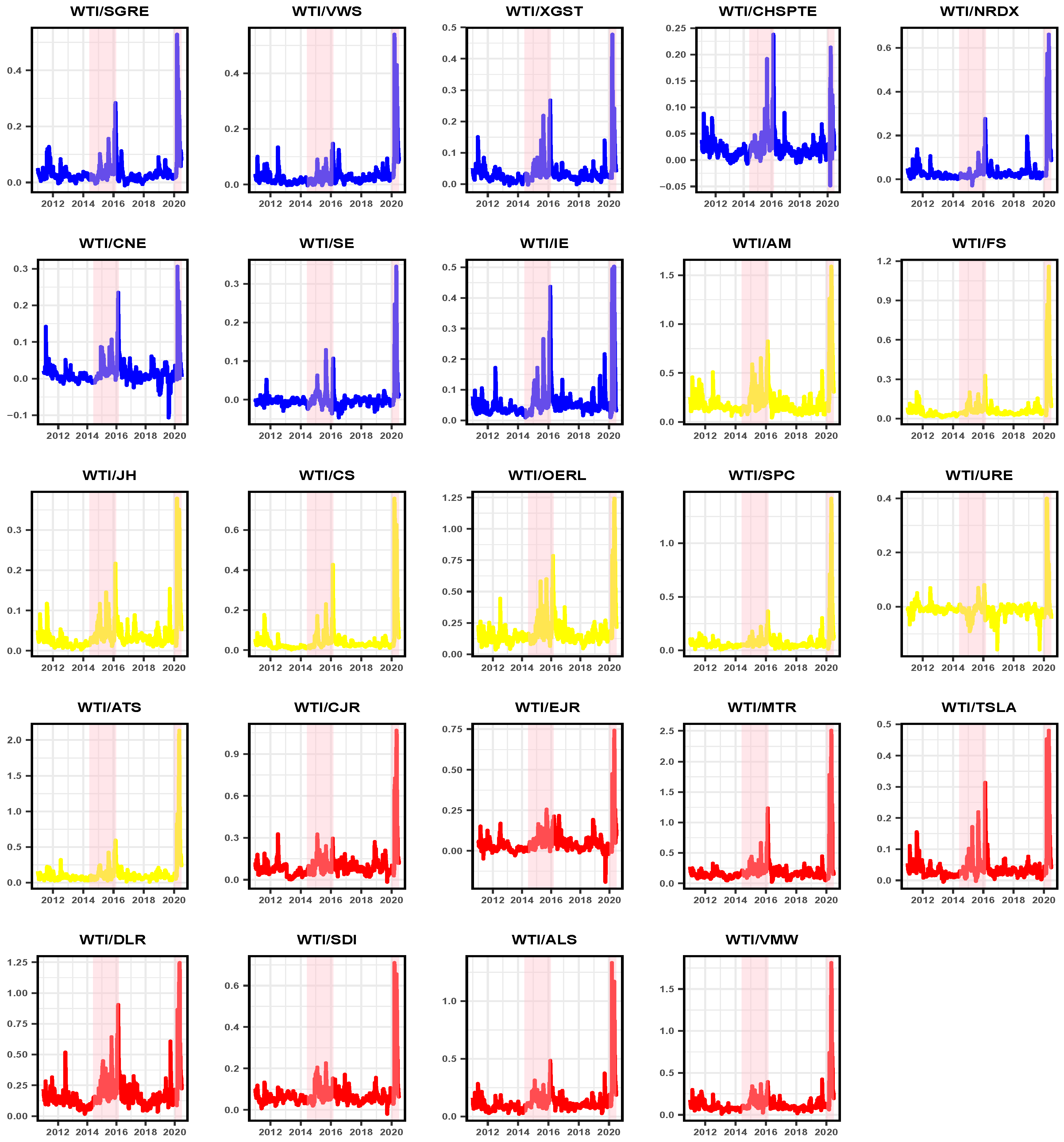
5.2.1. Hedging
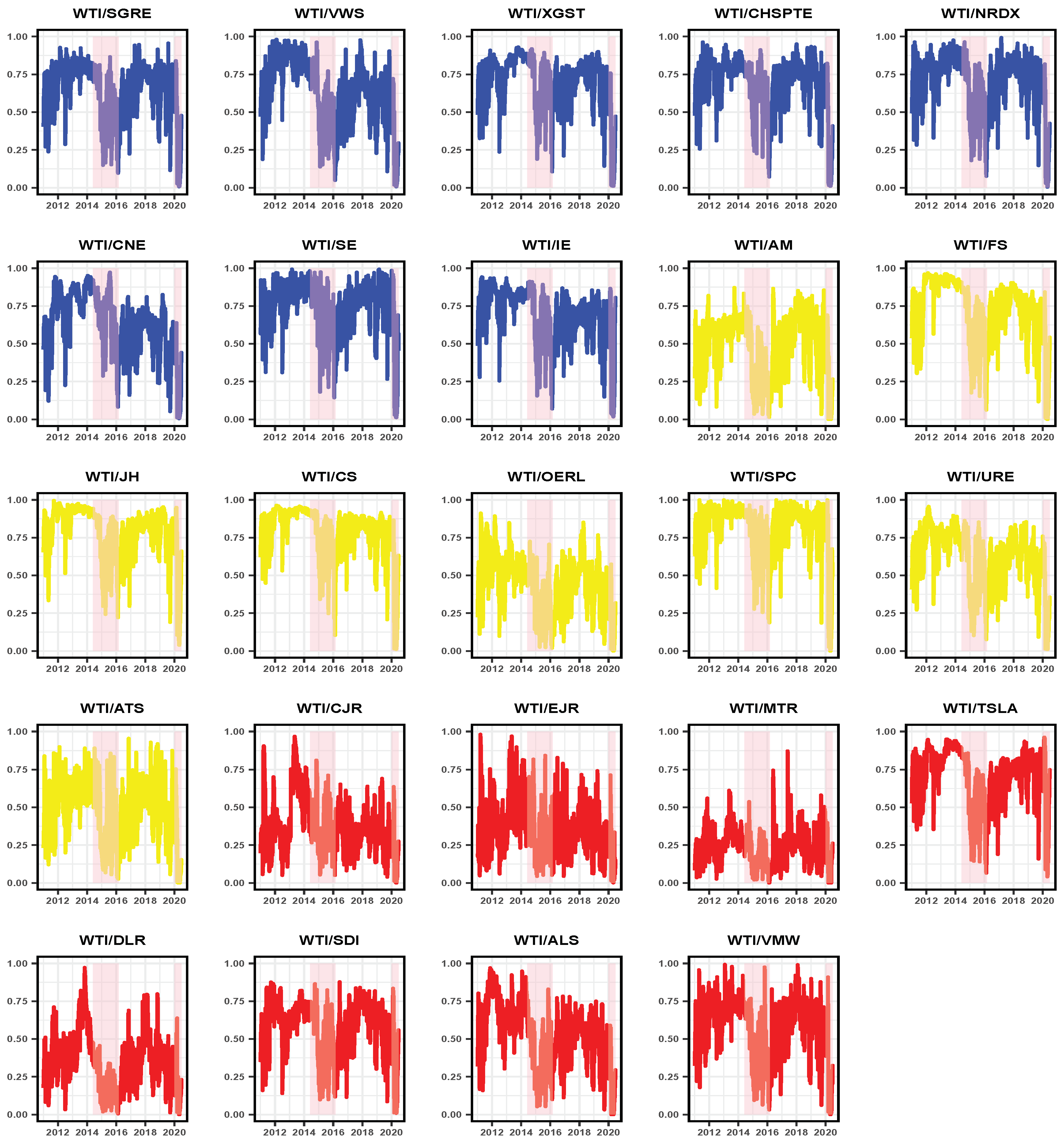
5.2.2. Optimal Portfolio Weight
6. Conclusions
Author Contributions
Funding
Conflicts of Interest
References
- Henriques, I.; Sadorsky, P. Oil prices and the stock prices of alternative energy companies. Energy Econ. 2008, 30, 998–1010. [Google Scholar] [CrossRef]
- Sadorsky, P. Correlations and volatility spillovers between oil prices and the stock prices of clean energy and technology companies. Energy Econ. 2012, 34, 248–255. [Google Scholar] [CrossRef]
- Managi, S.; Okimoto, T. Does the price of oil interact with clean energy prices in the stock market? Jpn. World Econ. 2013, 27, 1–9. [Google Scholar] [CrossRef]
- Reboredo, J.C. Is there dependence and systemic risk between oil and renewable energy stock prices? Energy Econ. 2015, 48, 32–45. [Google Scholar] [CrossRef]
- Reboredo, J.C.; Rivera-Castro, M.A.; Ugolini, A. Wavelet-based test of co-movement and causality between oil and renewable energy stock prices. Energy Econ. 2017, 61, 241–252. [Google Scholar] [CrossRef]
- Pham, L. Do all clean energy stocks respond homogeneously to oil price? Energy Econ. 2019, 81, 355–379. [Google Scholar] [CrossRef]
- Maghyereh, A.I.; Awartani, B.; Abdoh, H. The co-movement between oil and clean energy stocks: A wavelet-based analysis of horizon associations. Energy 2019, 169, 895–913. [Google Scholar] [CrossRef]
- Zhang, H.; Cai, G.; Yang, D. The impact of oil price shocks on clean energy stocks: Fresh evidence from multi-scale perspective. Energy 2020, 196, 117099. [Google Scholar] [CrossRef]
- Kumar, S.; Managi, S.; Matsuda, A. Stock prices of clean energy firms, oil and carbon markets: A vector autoregressive analysis. Energy Econ. 2012, 34, 215–226. [Google Scholar] [CrossRef]
- Haixia, W.; Shiping, L. Volatility spillovers in China’s crude oil, corn and fuel ethanol markets. Energy Policy 2013, 62, 878–886. [Google Scholar] [CrossRef]
- Inchauspe, J.; Ripple, R.D.; Trück, S. The dynamics of returns on renewable energy companies: A state-space approach. Energy Econ. 2015, 48, 325–335. [Google Scholar] [CrossRef]
- Li, H.; An, H.; Liu, X.; Gao, X.; Fang, W.; An, F. Price fluctuation in the energy stock market based on fluctuation and co-fluctuation matrix transmission networks. Energy 2016, 117, 73–83. [Google Scholar] [CrossRef]
- Dutta, A. Oil price uncertainty and clean energy stock returns: New evidence from crude oil volatility index. J. Clean. Prod. 2017, 164, 1157–1166. [Google Scholar] [CrossRef]
- Ferrer, R.; Shahzad, S.J.H.; López, R.; Jareño, F. Time and frequency dynamics of connectedness between renewable energy stocks and crude oil prices. Energy Econ. 2018, 76, 1–20. [Google Scholar] [CrossRef]
- Dutta, A.; Bouri, E.; Noor, M.H. Return and volatility linkages between CO2 emission and clean energy stock prices. Energy 2018, 164, 803–810. [Google Scholar] [CrossRef]
- Shahzad, S.J.H.; Hernandez, J.A.; Al-Yahyaee, K.H.; Jammazi, R. Asymmetric risk spillovers between oil and agricultural commodities. Energy Policy 2018, 118, 182–198. [Google Scholar] [CrossRef]
- Uddin, G.S.; Rahman, M.L.; Hedström, A.; Ahmed, A. Cross-quantilogram-based correlation and dependence between renewable energy stock and other asset classes. Energy Econ. 2019, 80, 743–759. [Google Scholar] [CrossRef]
- Ji, Q.; Du, Y.J.; Geng, J.B. The dynamic dependence of fossil energy, investor sentiment and renewable energy stock markets. Energy Econ. 2019, 84, 104564. [Google Scholar]
- Yahya, M.; Ghosh, S.; Kanjilal, K.; Dutta, A.; Uddin, G.S. Evaluation of cross-quantile dependence and causality between non-ferrous metals and clean energy indexes. Energy 2020, 202, 117777. [Google Scholar] [CrossRef]
- Rizwan, M.S.; Ahmad, G.; Ashraf, D. Systemic Risk: The Impact of COVID-19. Finace Res. Lett. 2020, 36, 101682. [Google Scholar] [CrossRef]
- Ashraf, B.N. Stock markets’ reaction to COVID-19: Cases or fatalities? Res. Int. Bus. Financ. 2020, 54, 101249. [Google Scholar] [CrossRef]
- Ahmad, W.; Sadorsky, P.; Sharma, A. Optimal hedge ratios for clean energy equities. Econ. Model. 2018, 72, 278–295. [Google Scholar] [CrossRef]
- Bondia, R.; Ghosh, S.; Kanjilal, K. International crude oil prices and the stock prices of clean energy and technology companies: Evidence from non-linear cointegration tests with unknown structural breaks. Energy 2016, 101, 558–565. [Google Scholar] [CrossRef]
- Antonakakis, N.; Cunado, J.; Filis, G.; Gabauer, D.; De Gracia, F.P. Oil volatility, oil and gas firms and portfolio diversification. Energy Econ. 2018, 70, 499–515. [Google Scholar] [CrossRef]
- Mandacı, P.E.; Cagli, E.Ç.; Taşkın, D. Dynamic connectedness and portfolio strategies: Energy and metal markets. Resour. Policy 2020, 68, 101778. [Google Scholar] [CrossRef]
- Diebold, F.X.; Yılmaz, K. Better to give than to receive: Predictive directional measurement of volatility spillovers. Int. J. Forecast. 2012, 28, 57–66. [Google Scholar] [CrossRef]
- Diebold, F.X.; Yılmaz, K. On the network topology of variance decompositions: Measuring the connectedness of financial firms. J. Econom. 2014, 182, 119–134. [Google Scholar] [CrossRef]
- Engle, R. Dynamic conditional correlation: A simple class of multivariate generalized autoregressive conditional heteroskedasticity models. J. Bus. Econ. Stat. 2002, 20, 339–350. [Google Scholar] [CrossRef]
- Ahmad, W. On the dynamic dependence and investment performance of crude oil and clean energy stocks. Res. Int. Bus. Financ. 2017, 42, 376–389. [Google Scholar] [CrossRef]
- Nasreen, S.; Tiwari, A.K.; Eizaguirre, J.C.; Wohar, M.E. Dynamic connectedness between oil prices and stock returns of clean energy and technology companies. J. Clean. Prod. 2020, 260, 121015. [Google Scholar] [CrossRef]
- Nazlioglu, S.; Soytas, U.; Gupta, R. Oil prices and financial stress: A volatility spillover analysis. Energy Policy 2015, 82, 278–288. [Google Scholar] [CrossRef]
- Reboredo, J.C.; Ugolini, A. The impact of energy prices on clean energy stock prices. A multivariate quantile dependence approach. Energy Econ. 2018, 76, 136–152. [Google Scholar] [CrossRef]
- Forsberg, L.; Ghysels, E. Why do absolute returns predict volatility so well? J. Financ. Econom. 2007, 5, 31–67. [Google Scholar] [CrossRef]
- Wang, G.J.; Xie, C.; Jiang, Z.Q.; Stanley, H.E. Who are the net senders and recipients of volatility spillovers in China’s financial markets? Financ. Res. Lett. 2016, 18, 255–262. [Google Scholar] [CrossRef]
- Koop, G.; Pesaran, M.H.; Potter, S.M. Impulse response analysis in nonlinear multivariate models. J. Econom. 1996, 74, 119–147. [Google Scholar] [CrossRef]
- Pesaran, H.H.; Shin, Y. Generalized impulse response analysis in linear multivariate models. Econ. Lett. 1998, 58, 17–29. [Google Scholar] [CrossRef]
- Awartani, B.; Aktham, M.; Cherif, G. The connectedness between crude oil and financial markets: Evidence from implied volatility indices. J. Commod. Mark. 2016, 4, 56–69. [Google Scholar] [CrossRef]
- Maghyereh, A.I.; Awartani, B.; Bouri, E. The directional volatility connectedness between crude oil and equity markets: New evidence from implied volatility indexes. Energy Econ. 2016, 57, 78–93. [Google Scholar] [CrossRef]
- Restrepo, N.; Uribe, J.M.; Manotas, D. Financial risk network architecture of energy firms. Appl. Energy 2018, 215, 630–642. [Google Scholar] [CrossRef]
- Lundgren, A.I.; Milicevic, A.; Uddin, G.S.; Kang, S.H. Connectedness network and dependence structure mechanism in green investments. Energy Econ. 2018, 72, 145–153. [Google Scholar] [CrossRef]
- Baldi, L.; Peri, M.; Vandone, D. Clean energy industries and rare earth materials: Economic and financial issues. Energy Policy 2014, 66, 53–61. [Google Scholar] [CrossRef]
- Dutta, A.; Bouri, E.; Uddin, G.S.; Yahya, M. Impact of COVID-19 on Global Energy Markets. IAEE Energy Forum 2020, 26–29. [Google Scholar]
- Sharif, A.; Aloui, C.; Yarovaya, L. COVID-19 pandemic, oil prices, stock market, geopolitical risk and policy uncertainty nexus in the US economy: Fresh evidence from the wavelet-based approach. Int. Rev. Financ. Anal. 2020, 70, 101496. [Google Scholar] [CrossRef]
- Kazemilari, M.; Mardani, A.; Streimikiene, D.; Zavadskas, E.K. An overview of renewable energy companies in stock exchange: Evidence from minimal spanning tree approach. Renew. Energy 2017, 102, 107–117. [Google Scholar] [CrossRef]
- Kim, B.; Kim, J.; Kim, J. Evaluation model for investment in solar photovoltaic power generation using fuzzy analytic hierarchy process. Sustainability 2019, 11, 2905. [Google Scholar] [CrossRef]
- Kroner, K.F.; Sultan, J. Time-varying distributions and dynamic hedging with foreign currency futures. J. Financ. Quant. Anal. 1993, 28, 535–551. [Google Scholar] [CrossRef]
- Kroner, K.; Ng, V. Modeling asymmetric movement of asset prices. Rev. Financ. Stud. 1998, 11, 844–871. [Google Scholar] [CrossRef]
- Antonakakis, N.; Chatziantoniou, I.; Gabauer, D. Refined measures of dynamic connectedness based on time-varying parameter vector autoregressions. J. Risk Financ. Manag. 2020, 13, 84. [Google Scholar] [CrossRef]


| Company | Abbr. | Total Asset (2019) |
|---|---|---|
| Panel A: Wind | ||
| Siemens Gamesa Renewable Energy, S.A. | SGRE | 18.17 |
| Vestas Wind Systems A/S | VWS | 16.10 |
| Xinjiang Goldwind Science & Technology Co. Ltd. | XGST | 11.87 |
| China High Speed Transmission Equipment Group Co Ltd. | CHSPTE | 3.90 |
| Nordex Se | NRDX | 3.50 |
| Concord New Energy Group Limited | CNE | 2.69 |
| Suzlon Energy Limited | SE | 1.28 |
| Infigen Energy | IE | 0.88 |
| Panel B: Solar | ||
| Applied Materials Inc. | AM | 19.02 |
| First Solar, Inc. | FS | 7.52 |
| Jinkosolar Holding Co., Ltd. | JH | 5.23 |
| Canadian Solar Inc. | CS | 4.89 |
| Oc Oerlikon Corporation Ag | OERL | 4.62 |
| Sunpower Corporation | SPC | 2.17 |
| United Renewable Energy Co., Ltd. | URE | 1.90 |
| Ats Automation Tooling Systems Inc. | ATS | 1.26 |
| Panel C: Clean Tech | ||
| Central Japan Railway Company | CJR | 83.81 |
| East Japan Railway Company | EJR | 75.36 |
| MTR Corporation Limited | MTR | 35.06 |
| Tesla, Inc. | TSLA | 34.31 |
| Digital Realty Trust, Inc. | DLR | 23.76 |
| Samsung SDI Co., Ltd. | SDI | 17.30 |
| Alstom S.A. | ALS | 15.06 |
| Vmware, Inc. | VMW | 14.66 |
| Mean | Median | Max | Min | Std.Dev | Skewness | Kurtosis | ADF | JB | |
|---|---|---|---|---|---|---|---|---|---|
| SGRE | 1.94 | 1.37 | 19.42 | 0.00 | 1.99 | 2.66 | 15.52 | −11.09 *** | 18156 *** |
| VWS | 1.98 | 1.30 | 27.82 | 0.00 | 2.23 | 3.31 | 23.22 | −10.03 *** | 44402 *** |
| XGST | 2.26 | 1.62 | 24.72 | 0.00 | 2.31 | 2.28 | 12.21 | −9.557 *** | 10355 *** |
| CHSPTE | 2.10 | 1.44 | 21.48 | 0.00 | 2.28 | 2.49 | 12.69 | −9.714 *** | 11647 *** |
| NRDX | 2.19 | 1.56 | 28.75 | 0.00 | 2.36 | 2.98 | 19.03 | −10.85 *** | 28688 *** |
| CNE | 1.97 | 1.46 | 22.56 | 0.00 | 2.19 | 2.41 | 13.65 | −9.069 *** | 13400 *** |
| SE | 2.55 | 1.79 | 41.58 | 0.00 | 2.95 | 3.52 | 28.23 | −10.45 *** | 67303 *** |
| IE | 2.17 | 1.78 | 31.07 | 0.00 | 2.33 | 2.48 | 17.39 | −10.55 *** | 22730 *** |
| AM | 1.51 | 1.08 | 22.76 | 0.00 | 1.59 | 3.32 | 25.85 | −7.655 *** | 55552 *** |
| FS | 2.30 | 1.58 | 37.52 | 0.00 | 2.56 | 3.73 | 31.51 | −10.11 *** | 85232 *** |
| JH | 3.35 | 2.46 | 34.26 | 0.00 | 3.20 | 2.40 | 14.11 | −9.121 *** | 14368 *** |
| CS | 2.87 | 2.00 | 28.88 | 0.00 | 3.00 | 2.53 | 12.79 | −9.717 *** | 11905 *** |
| OERL | 1.35 | 0.95 | 11.78 | 0.00 | 1.40 | 2.42 | 12.31 | −8.702 *** | 10812 *** |
| SPC | 2.88 | 2.10 | 39.18 | 0.00 | 3.05 | 3.37 | 25.30 | −10.38 *** | 53240 *** |
| URE | 1.88 | 1.25 | 17.25 | 0.00 | 1.97 | 1.82 | 7.55 | −10.14 *** | 3327 *** |
| ATS | 1.30 | 0.89 | 12.44 | 0.00 | 1.39 | 2.70 | 14.45 | −9.429 *** | 15713 *** |
| CJR | 1.09 | 0.76 | 18.74 | 0.00 | 1.23 | 3.72 | 33.16 | −8.163 *** | 94674 *** |
| EJR | 1.04 | 0.77 | 20.27 | 0.00 | 1.14 | 4.68 | 55.60 | −9.038 *** | 280133 *** |
| MTR | 0.81 | 0.59 | 10.35 | 0.00 | 0.83 | 3.04 | 23.41 | −8.961 *** | 44510 *** |
| TSLA | 2.28 | 1.62 | 21.83 | 0.00 | 2.51 | 2.93 | 15.93 | −8.896 *** | 19792 *** |
| DLR | 1.12 | 0.80 | 16.57 | 0.00 | 1.21 | 3.72 | 28.87 | −8.154 *** | 71087 *** |
| SDI | 1.68 | 1.19 | 19.09 | 0.00 | 1.79 | 2.60 | 15.54 | −9.211 *** | 18095 *** |
| ALS | 1.51 | 1.03 | 14.23 | 0.00 | 1.70 | 2.55 | 12.57 | −7.854 *** | 11539 *** |
| VMW | 1.53 | 1.08 | 24.26 | 0.00 | 1.73 | 4.10 | 34.79 | −8.788 *** | 105754 *** |
| WTI | 1.69 | 1.10 | 39.47 | 0.00 | 2.36 | 6.71 | 75.41 | −7.356 *** | 532221 *** |
| SGRE | VWS | XGST | CHSPTE | NRDX | CNE | SE | IE | AM | FS | JH | CS | OERL | SPC | URE | ATS | CJR | EJR | MTR | TSLA | DLR | SDI | ALS | VMW | WTI | FROM | |
|---|---|---|---|---|---|---|---|---|---|---|---|---|---|---|---|---|---|---|---|---|---|---|---|---|---|---|
| SGRE | 71.77 | 8.26 | 0.2 | 0.4 | 3.39 | 0.57 | 0.04 | 0.17 | 1.31 | 0.78 | 1.07 | 1.32 | 2.71 | 0.77 | 0.54 | 0.84 | 0.32 | 0.42 | 0.23 | 0.44 | 0.8 | 0.25 | 2.7 | 0.69 | 0.02 | 28.23 |
| VWS | 8.2 | 75.25 | 0.13 | 0.53 | 2.66 | 0.56 | 0.14 | 0.66 | 0.21 | 0.93 | 1.04 | 1.57 | 1.41 | 0.37 | 0.75 | 1.21 | 0.24 | 0.37 | 0.04 | 0.53 | 0.35 | 0.22 | 2.19 | 0.37 | 0.08 | 24.75 |
| XGST | 0.12 | 0.15 | 75.64 | 9.7 | 0.58 | 3.87 | 0.04 | 0.4 | 0.5 | 0.22 | 1.21 | 1.39 | 0.36 | 0.09 | 0.77 | 0.26 | 0.52 | 0.72 | 1.09 | 0.14 | 1 | 0.22 | 0.44 | 0.34 | 0.22 | 24.36 |
| CHSPTE | 0.11 | 0.2 | 9.76 | 77.82 | 0.21 | 4.13 | 0.06 | 0.05 | 0.61 | 0.33 | 0.66 | 0.89 | 0.21 | 0.27 | 1.02 | 0.05 | 0.23 | 0.09 | 1.33 | 0.22 | 0.32 | 0.13 | 1.05 | 0.22 | 0.02 | 22.18 |
| NRDX | 3.55 | 3.5 | 0.69 | 0.35 | 75.77 | 0.59 | 0.21 | 0.34 | 1.89 | 0.42 | 0.89 | 1.29 | 1.93 | 0.5 | 0.32 | 0.58 | 0.97 | 1.61 | 0.53 | 0.84 | 1.28 | 0.2 | 1.24 | 0.48 | 0.06 | 24.23 |
| CNE | 0.32 | 0.26 | 4.26 | 4.99 | 0.41 | 82.98 | 0.2 | 0.4 | 0.03 | 0.23 | 0.42 | 1.37 | 0.18 | 0.13 | 0.35 | 0.33 | 0.16 | 0.15 | 1.46 | 0.01 | 0.19 | 0.15 | 0.94 | 0.04 | 0.05 | 17.02 |
| SE | 0.06 | 0.25 | 0.04 | 0.14 | 0.26 | 0.23 | 96.79 | 0.03 | 0.25 | 0.1 | 0.11 | 0.2 | 0.39 | 0 | 0.03 | 0.26 | 0.09 | 0.03 | 0.2 | 0.12 | 0.11 | 0.03 | 0.24 | 0 | 0.03 | 3.21 |
| IE | 0.6 | 0.78 | 0.21 | 0.24 | 0.62 | 0.38 | 0.02 | 87.43 | 0.6 | 0.17 | 0.37 | 0.26 | 1.42 | 0.1 | 0.39 | 0.69 | 0.46 | 0.46 | 0.53 | 0.32 | 0.5 | 0.66 | 1.3 | 0.49 | 1.01 | 12.57 |
| AM | 1.3 | 0.41 | 0.25 | 0.28 | 1.7 | 0.02 | 0.12 | 0.24 | 61.76 | 1.22 | 2.01 | 2.12 | 2.35 | 2.7 | 0.3 | 2.91 | 0.43 | 0.41 | 1.34 | 2.65 | 4.73 | 0.49 | 2.46 | 4.86 | 2.94 | 38.24 |
| FS | 0.86 | 1.71 | 0.21 | 0.09 | 0.13 | 0.24 | 0.02 | 0.07 | 1.25 | 65.5 | 5.64 | 6.32 | 0.76 | 9.93 | 0.68 | 0.48 | 0.17 | 0.25 | 0.07 | 0.62 | 1.13 | 0.07 | 2.22 | 1.2 | 0.38 | 34.5 |
| JH | 0.96 | 1.28 | 0.94 | 0.39 | 0.79 | 0.74 | 0.15 | 0.33 | 2.36 | 4.86 | 59.41 | 14.88 | 0.66 | 5.55 | 0.81 | 0.78 | 0.22 | 0.5 | 0.5 | 0.84 | 0.69 | 0.1 | 1.62 | 0.56 | 0.07 | 40.59 |
| CS | 0.73 | 1.23 | 1.05 | 0.35 | 0.87 | 1.56 | 0.09 | 0.25 | 2.15 | 5.49 | 13.8 | 55.71 | 1.52 | 6.83 | 1.03 | 1.03 | 0.47 | 0.66 | 0.48 | 0.74 | 0.77 | 0.16 | 2.07 | 0.84 | 0.13 | 44.29 |
| OERL | 2.43 | 1.8 | 0.26 | 0.31 | 1.95 | 0.35 | 0.28 | 1.21 | 2.83 | 1.18 | 1.19 | 1.74 | 67.98 | 1.77 | 0.38 | 1.04 | 0.87 | 0.99 | 1.37 | 0.64 | 1.2 | 0.8 | 4.66 | 1.75 | 1 | 32.02 |
| SPC | 0.77 | 0.69 | 0.05 | 0.07 | 0.28 | 0.09 | 0.01 | 0.05 | 2.86 | 9.95 | 6.19 | 7.54 | 1.52 | 62.86 | 0.24 | 0.81 | 0.1 | 0.32 | 0.49 | 1.02 | 1.19 | 0.1 | 1.31 | 0.67 | 0.84 | 37.14 |
| URE | 0.66 | 0.76 | 1.15 | 0.71 | 0.93 | 0.84 | 0.02 | 0.31 | 0.91 | 0.79 | 1.26 | 1.36 | 0.83 | 0.37 | 81.79 | 1.15 | 0.47 | 0.35 | 0.41 | 0.43 | 0.82 | 0.96 | 1.95 | 0.68 | 0.06 | 18.21 |
| ATS | 1.29 | 1.77 | 0.23 | 0.03 | 0.76 | 0.31 | 0.22 | 0.16 | 3.08 | 0.54 | 0.56 | 1.4 | 1.21 | 0.53 | 0.67 | 78.95 | 0.53 | 0.42 | 0.37 | 0.57 | 1.65 | 0.16 | 2.51 | 1.02 | 1.02 | 21.05 |
| CJR | 0.81 | 0.5 | 0.65 | 0.29 | 1.23 | 0.39 | 0.1 | 0.38 | 0.98 | 0.17 | 0.65 | 1.02 | 1.03 | 0.76 | 0.4 | 0.57 | 59.46 | 26.29 | 0.86 | 0.46 | 1.66 | 0.06 | 0.48 | 0.4 | 0.42 | 40.54 |
| EJR | 0.57 | 0.24 | 0.29 | 0.17 | 0.73 | 0.27 | 0.17 | 0.37 | 1.01 | 0.1 | 0.56 | 0.95 | 0.69 | 0.77 | 0.36 | 0.88 | 25.73 | 63.51 | 0.31 | 0.19 | 0.99 | 0.05 | 0.52 | 0.23 | 0.31 | 36.49 |
| MTR | 0.17 | 0.09 | 1.21 | 1.37 | 0.39 | 1.7 | 0.22 | 0.42 | 1.85 | 0.14 | 0.65 | 0.81 | 1.3 | 0.5 | 0.44 | 0.86 | 0.93 | 0.47 | 80.47 | 0.48 | 1.31 | 0.69 | 0.92 | 0.69 | 1.92 | 19.53 |
| TSLA | 0.45 | 0.69 | 0.06 | 0.04 | 0.94 | 0.01 | 0.08 | 0.16 | 4.46 | 0.88 | 1.37 | 1.2 | 0.78 | 1.41 | 0.4 | 0.34 | 0.31 | 0.52 | 0.39 | 79.97 | 1.65 | 0.16 | 1.4 | 1.44 | 0.89 | 20.03 |
| DLR | 0.9 | 0.87 | 0.38 | 0.16 | 1.45 | 0.16 | 0.06 | 0.58 | 5.71 | 0.6 | 0.8 | 0.89 | 2.07 | 1.27 | 0.82 | 2.57 | 0.93 | 0.47 | 0.93 | 1.65 | 68.29 | 1.01 | 1.98 | 3.49 | 1.97 | 31.71 |
| SDI | 0.76 | 0.16 | 0.36 | 0.15 | 0.3 | 0.18 | 0.04 | 0.46 | 2.15 | 0.14 | 0.37 | 0.12 | 1.47 | 0.1 | 0.75 | 0.58 | 0.2 | 0.09 | 0.51 | 0.56 | 2.36 | 85.27 | 1.87 | 0.5 | 0.54 | 14.73 |
| ALS | 2.31 | 1.82 | 0.33 | 0.67 | 1.15 | 1.07 | 0.16 | 0.58 | 2.9 | 2.4 | 1.71 | 2.58 | 4.45 | 1.27 | 0.94 | 2.53 | 0.32 | 0.37 | 0.33 | 1.36 | 1.74 | 0.85 | 65.22 | 1.95 | 1.03 | 34.78 |
| VMW | 1.01 | 0.76 | 0.04 | 0.16 | 0.64 | 0.04 | 0.01 | 0.21 | 6.35 | 1.67 | 0.7 | 1.26 | 2.1 | 0.95 | 0.49 | 0.66 | 0.17 | 0.23 | 0.17 | 1.41 | 3.37 | 0.21 | 2.32 | 74.21 | 0.86 | 25.79 |
| WTI | 0.14 | 0.06 | 0.14 | 0.03 | 0.22 | 0.01 | 0.08 | 0.69 | 5.06 | 1.06 | 0.24 | 0.46 | 1.89 | 1.24 | 0.05 | 1.33 | 0.74 | 1.13 | 0.51 | 2.02 | 2.53 | 0.83 | 1.15 | 0.83 | 77.55 | 22.45 |
| TO | 29.09 | 28.24 | 22.87 | 21.6 | 22.59 | 18.32 | 2.56 | 8.5 | 51.3 | 34.37 | 43.48 | 52.9 | 33.23 | 38.18 | 12.93 | 22.76 | 35.6 | 37.32 | 14.46 | 18.26 | 32.34 | 8.57 | 39.53 | 23.73 | 15.87 | |
| ALL | 100.87 | 103.5 | 98.51 | 99.42 | 98.35 | 101.3 | 99.35 | 95.93 | 113.07 | 99.87 | 102.89 | 108.61 | 101.2 | 101.05 | 94.73 | 101.71 | 95.06 | 100.83 | 94.93 | 98.24 | 100.63 | 93.83 | 104.75 | 97.94 | 93.42 | TCI |
| NET | 0.87 | 3.5 | −1.49 | −0.58 | −1.65 | 1.3 | −0.65 | −4.07 | 13.07 | −0.13 | 2.89 | 8.61 | 1.2 | 1.05 | −5.27 | 1.71 | −4.94 | 0.83 | −5.07 | −1.76 | 0.63 | −6.17 | 4.75 | −2.06 | −6.58 | 26.74 |
| SGRE | VWS | XGST | CHSPTE | NRDX | CNE | SE | IE | AM | FS | JH | CS | OERL | SPC | URE | ATS | CJR | EJR | MTR | TSLA | DLR | SDI | ALS | VMW | WTI | FROM | |
|---|---|---|---|---|---|---|---|---|---|---|---|---|---|---|---|---|---|---|---|---|---|---|---|---|---|---|
| SGRE | 76.21 | 8.26 | 0.15 | 0.46 | 2.58 | 0.64 | 0.04 | 0.27 | 0.58 | 0.86 | 0.79 | 1 | 2.13 | 0.39 | 0.42 | 0.66 | 0.28 | 0.42 | 0.04 | 0.1 | 0.31 | 0.18 | 2.44 | 0.62 | 0.18 | 23.79 |
| VWS | 8.01 | 77.69 | 0.07 | 0.58 | 2.02 | 0.56 | 0.15 | 0.66 | 0.08 | 0.92 | 1.03 | 1.56 | 1.05 | 0.26 | 0.67 | 1.11 | 0.2 | 0.45 | 0.09 | 0.29 | 0.16 | 0.12 | 1.9 | 0.33 | 0.04 | 22.31 |
| XGST | 0.08 | 0.08 | 75.44 | 9.82 | 0.51 | 3.92 | 0.07 | 0.24 | 0.49 | 0.27 | 1.26 | 1.43 | 0.39 | 0.15 | 0.71 | 0.21 | 0.7 | 0.93 | 0.79 | 0.07 | 1.22 | 0.25 | 0.31 | 0.28 | 0.39 | 24.56 |
| CHSPTE | 0.07 | 0.2 | 9.69 | 75.67 | 0.28 | 3.96 | 0.17 | 0.05 | 1.12 | 0.41 | 0.75 | 0.91 | 0.38 | 0.42 | 1.02 | 0.05 | 0.41 | 0.14 | 1.32 | 0.24 | 0.65 | 0.24 | 1.33 | 0.28 | 0.21 | 24.33 |
| NRDX | 2.74 | 2.88 | 0.69 | 0.49 | 83.83 | 0.67 | 0.15 | 0.12 | 0.6 | 0.34 | 0.44 | 1.02 | 0.97 | 0.18 | 0.17 | 0.3 | 0.7 | 1.77 | 0.15 | 0.29 | 0.37 | 0.12 | 0.72 | 0.21 | 0.09 | 16.17 |
| CNE | 0.33 | 0.23 | 4.25 | 4.81 | 0.39 | 81.73 | 0.36 | 0.5 | 0.01 | 0.31 | 0.62 | 1.55 | 0.24 | 0.17 | 0.37 | 0.34 | 0.21 | 0.18 | 1.54 | 0.01 | 0.41 | 0.23 | 1.07 | 0.08 | 0.07 | 18.27 |
| SE | 0.06 | 0.27 | 0.04 | 0.27 | 0.17 | 0.36 | 96.97 | 0.01 | 0.09 | 0.13 | 0.06 | 0.21 | 0.27 | 0.02 | 0.05 | 0.2 | 0.07 | 0.02 | 0.25 | 0.05 | 0.04 | 0.03 | 0.17 | 0.01 | 0.2 | 3.03 |
| IE | 0.57 | 0.69 | 0.21 | 0.22 | 0.33 | 0.41 | 0.02 | 91.47 | 0.08 | 0.14 | 0.12 | 0.16 | 1.06 | 0.01 | 0.22 | 0.3 | 0.31 | 0.3 | 0.28 | 0.04 | 0.18 | 0.41 | 1.12 | 0.25 | 1.11 | 8.53 |
| AM | 0.68 | 0.16 | 0.47 | 0.9 | 0.73 | 0 | 0.05 | 0.03 | 79.23 | 0.91 | 1.06 | 1.25 | 1.13 | 1.6 | 0.03 | 0.74 | 0.06 | 0.04 | 1.33 | 1.21 | 0.9 | 0.34 | 1.87 | 3.67 | 1.63 | 20.77 |
| FS | 1.01 | 1.84 | 0.27 | 0.14 | 0.11 | 0.3 | 0.04 | 0.04 | 0.74 | 67.6 | 5.53 | 5.98 | 0.65 | 10.3 | 0.73 | 0.32 | 0.06 | 0.11 | 0.02 | 0.31 | 0.76 | 0.06 | 1.96 | 0.9 | 0.21 | 32.4 |
| JH | 0.77 | 1.31 | 1.11 | 0.55 | 0.48 | 1 | 0.09 | 0.19 | 0.94 | 4.85 | 63.91 | 14.61 | 0.45 | 5.13 | 0.73 | 0.32 | 0.2 | 0.5 | 0.39 | 0.28 | 0.21 | 0.09 | 1.43 | 0.25 | 0.21 | 36.09 |
| CS | 0.57 | 1.23 | 1.2 | 0.45 | 0.69 | 1.83 | 0.09 | 0.26 | 0.98 | 5.31 | 13.54 | 59.45 | 1.26 | 6.59 | 0.89 | 0.6 | 0.42 | 0.55 | 0.47 | 0.45 | 0.34 | 0.18 | 1.97 | 0.49 | 0.2 | 40.55 |
| OERL | 1.97 | 1.43 | 0.33 | 0.6 | 1 | 0.48 | 0.21 | 1.14 | 1.2 | 0.95 | 1.01 | 1.46 | 76.02 | 0.9 | 0.21 | 0.65 | 0.58 | 1.04 | 0.88 | 0.17 | 0.39 | 0.53 | 4.23 | 1.03 | 1.61 | 23.98 |
| SPC | 0.59 | 0.75 | 0.11 | 0.15 | 0.08 | 0.15 | 0.02 | 0.01 | 1.33 | 10.6 | 5.71 | 7.29 | 0.76 | 67.84 | 0.2 | 0.43 | 0.02 | 0.24 | 0.45 | 0.51 | 0.52 | 0.02 | 1.03 | 0.35 | 0.85 | 32.16 |
| URE | 0.38 | 0.52 | 1.06 | 0.75 | 0.54 | 0.87 | 0.04 | 0.27 | 0.27 | 0.82 | 1.34 | 1.25 | 0.56 | 0.26 | 86.12 | 0.77 | 0.31 | 0.29 | 0.29 | 0.18 | 0.38 | 0.92 | 1.4 | 0.31 | 0.09 | 13.88 |
| ATS | 0.94 | 1.53 | 0.24 | 0.04 | 0.48 | 0.37 | 0.18 | 0.08 | 0.86 | 0.41 | 0.3 | 1.03 | 0.68 | 0.35 | 0.48 | 86.91 | 0.29 | 0.22 | 0.2 | 0.29 | 0.42 | 0.07 | 2.3 | 0.36 | 0.96 | 13.09 |
| CJR | 0.64 | 0.33 | 0.77 | 0.5 | 0.94 | 0.44 | 0.07 | 0.31 | 0.21 | 0.13 | 0.65 | 0.98 | 0.49 | 0.47 | 0.21 | 0.27 | 62.4 | 27.06 | 0.76 | 0.24 | 0.88 | 0.06 | 0.22 | 0.09 | 0.91 | 37.6 |
| EJR | 0.5 | 0.2 | 0.39 | 0.25 | 0.72 | 0.3 | 0.18 | 0.35 | 0.24 | 0.05 | 0.55 | 0.77 | 0.34 | 0.46 | 0.17 | 0.49 | 26.01 | 65.55 | 0.16 | 0.09 | 0.59 | 0.06 | 0.44 | 0.04 | 1.1 | 34.45 |
| MTR | 0.09 | 0.04 | 0.98 | 1.6 | 0.25 | 2.07 | 0.24 | 0.35 | 1.44 | 0.09 | 0.47 | 0.84 | 1.3 | 0.57 | 0.41 | 0.55 | 1.3 | 0.54 | 83.61 | 0.22 | 0.44 | 0.48 | 0.64 | 0.33 | 1.14 | 16.39 |
| TSLA | 0.12 | 0.51 | 0.04 | 0.11 | 0.29 | 0.01 | 0.07 | 0.04 | 1.43 | 0.48 | 0.68 | 0.8 | 0.24 | 0.67 | 0.27 | 0.05 | 0.11 | 0.24 | 0.23 | 91 | 0.6 | 0.07 | 0.83 | 0.74 | 0.36 | 9 |
| DLR | 0.39 | 0.36 | 0.55 | 0.46 | 0.55 | 0.37 | 0.02 | 0.16 | 1.26 | 0.42 | 0.44 | 0.58 | 1.01 | 0.6 | 0.43 | 0.64 | 0.42 | 0.23 | 0.32 | 0.63 | 85.49 | 0.34 | 1.16 | 2.05 | 1.09 | 14.51 |
| SDI | 0.32 | 0.13 | 0.41 | 0.28 | 0.15 | 0.23 | 0.02 | 0.32 | 1.07 | 0.06 | 0.22 | 0.05 | 0.85 | 0 | 0.67 | 0.3 | 0.06 | 0 | 0.31 | 0.03 | 0.74 | 92.15 | 0.88 | 0.32 | 0.45 | 7.85 |
| ALS | 2.06 | 1.49 | 0.27 | 0.96 | 0.57 | 1.23 | 0.13 | 0.45 | 1.53 | 2.22 | 1.46 | 2.49 | 4.01 | 0.93 | 0.89 | 2.31 | 0.18 | 0.32 | 0.13 | 0.74 | 0.94 | 0.55 | 71.18 | 1.72 | 1.22 | 28.82 |
| VMW | 0.84 | 0.62 | 0.06 | 0.28 | 0.26 | 0.05 | 0.01 | 0.09 | 4.08 | 1.33 | 0.35 | 0.87 | 1.29 | 0.56 | 0.27 | 0.19 | 0.04 | 0.07 | 0.06 | 0.72 | 1.81 | 0.15 | 2.02 | 83.08 | 0.89 | 16.92 |
| WTI | 0.21 | 0.01 | 0.47 | 0.24 | 0.06 | 0.18 | 0.12 | 0.89 | 1.61 | 0.26 | 0.25 | 0.29 | 1.83 | 1.08 | 0.14 | 0.7 | 0.9 | 1.12 | 0.6 | 0.13 | 0.93 | 0.18 | 1.45 | 0.78 | 85.58 | 14.42 |
| TO | 23.94 | 25.06 | 23.84 | 24.94 | 14.19 | 20.42 | 2.51 | 6.81 | 22.23 | 32.28 | 38.63 | 48.38 | 23.34 | 32.09 | 10.33 | 12.51 | 33.81 | 36.75 | 11.07 | 7.29 | 14.19 | 5.69 | 32.9 | 15.49 | 15.21 | |
| ALL | 100.14 | 102.76 | 99.27 | 100.61 | 98.02 | 102.15 | 99.47 | 98.28 | 101.46 | 99.88 | 102.53 | 107.83 | 99.36 | 99.92 | 96.45 | 99.42 | 96.21 | 102.3 | 94.68 | 98.29 | 99.68 | 97.84 | 104.08 | 98.57 | 100.79 | TCI |
| NET | 0.14 | 2.76 | −0.73 | 0.61 | −1.98 | 2.15 | −0.53 | −1.72 | 1.46 | −0.12 | 2.53 | 7.83 | −0.64 | −0.08 | −3.55 | −0.58 | −3.79 | 2.3 | −5.32 | −1.71 | −0.32 | −2.16 | 4.08 | −1.43 | 0.79 | 21.36 |
| SGRE | VWS | XGST | CHSPTE | NRDX | CNE | SE | IE | AM | FS | JH | CS | OERL | SPC | URE | ATS | CJR | EJR | MTR | TSLA | DLR | SDI | ALS | VMW | WTI | FROM | |
|---|---|---|---|---|---|---|---|---|---|---|---|---|---|---|---|---|---|---|---|---|---|---|---|---|---|---|
| SGRE | 34.5 | 8.78 | 2.22 | 0.43 | 6.86 | 0.46 | 0.25 | 0.15 | 6.94 | 2.54 | 2.9 | 5.22 | 3.36 | 3.65 | 1.02 | 2.22 | 0.68 | 0.88 | 3.25 | 3.37 | 4.21 | 0.79 | 3.11 | 1.02 | 1.19 | 65.5 |
| VWS | 6.48 | 26.5 | 6.14 | 0.36 | 9.28 | 0.84 | 2.32 | 1.26 | 3.74 | 1.64 | 3.09 | 1.62 | 4.38 | 1.76 | 1.17 | 2.43 | 0.5 | 0.37 | 4.95 | 4.5 | 2.76 | 3.39 | 6.77 | 0.79 | 2.97 | 73.5 |
| XGST | 1.32 | 5.62 | 37.87 | 0.75 | 4.97 | 0.5 | 0.82 | 5.12 | 4.16 | 0.89 | 1.79 | 1.42 | 0.97 | 0.32 | 2.23 | 2.47 | 0.94 | 1.54 | 10.05 | 4.03 | 2.02 | 0.6 | 5.02 | 1.95 | 2.65 | 62.13 |
| CHSPTE | 4.17 | 0.31 | 0.36 | 52.55 | 1.42 | 0.28 | 4.8 | 0.46 | 1.66 | 2.37 | 1.61 | 2.55 | 1.22 | 2.63 | 2.95 | 1.57 | 2.38 | 0.58 | 5.34 | 2.99 | 1.8 | 1.82 | 0.8 | 1.3 | 2.09 | 47.45 |
| NRDX | 6.09 | 10.46 | 5.1 | 0.53 | 25.68 | 0.95 | 1.89 | 2.08 | 4.22 | 1.71 | 3.55 | 1.85 | 6.02 | 1.78 | 1.87 | 2.07 | 0.83 | 0.8 | 4.27 | 4.87 | 4.38 | 1.77 | 5.5 | 1.22 | 0.52 | 74.32 |
| CNE | 0.96 | 1.92 | 1.11 | 0.99 | 2.36 | 70.03 | 0.57 | 0.26 | 0.41 | 3.81 | 2.34 | 0.84 | 0.27 | 0.61 | 0.3 | 2.57 | 0.18 | 0.24 | 6.88 | 1.27 | 0.68 | 0.64 | 0.25 | 0.19 | 0.31 | 29.97 |
| SE | 0.71 | 4.62 | 1.28 | 3.32 | 3.56 | 1.85 | 63.07 | 1.37 | 1.41 | 1.02 | 0.32 | 0.66 | 2.78 | 1.1 | 0.25 | 1.18 | 1.67 | 0.97 | 2.14 | 0.07 | 0.33 | 0.26 | 2.62 | 0.57 | 2.88 | 36.93 |
| IE | 1.07 | 2.62 | 2.77 | 2.13 | 4.57 | 1.76 | 0.25 | 53.45 | 1.85 | 3.21 | 5.56 | 2.3 | 2.07 | 1.43 | 1.9 | 1.61 | 0.14 | 0.51 | 2.93 | 1.47 | 0.93 | 0.46 | 3.18 | 1.36 | 0.5 | 46.55 |
| AM | 3.7 | 4.31 | 2.84 | 0.29 | 2.66 | 0.2 | 0.49 | 0.39 | 23.79 | 4.24 | 4.75 | 9.98 | 2.5 | 4.77 | 3.29 | 8.74 | 0.22 | 0.45 | 1.88 | 2.66 | 6.57 | 1.15 | 3.65 | 5.87 | 0.61 | 76.21 |
| FS | 1 | 0.37 | 0.67 | 1.36 | 0.41 | 2.06 | 0.34 | 2.34 | 5.63 | 38.24 | 6.16 | 10.57 | 1.45 | 6.18 | 0.6 | 1.57 | 1.51 | 1.85 | 1.5 | 1.75 | 3.74 | 0.32 | 2.81 | 5.78 | 1.77 | 61.76 |
| JH | 2.2 | 3.27 | 1.84 | 0.16 | 3.78 | 1.05 | 0.35 | 2.6 | 8.15 | 4.17 | 26.59 | 15.24 | 2.02 | 6.68 | 0.75 | 4.94 | 0.47 | 0.47 | 0.65 | 4.42 | 3.5 | 0.75 | 2.67 | 2.79 | 0.49 | 73.41 |
| CS | 2.4 | 1.99 | 1.35 | 0.17 | 1.45 | 0.41 | 0.33 | 0.99 | 12.92 | 7.4 | 13.23 | 24.04 | 2.55 | 7.48 | 1.27 | 5.68 | 0.45 | 0.68 | 0.84 | 2.19 | 4.47 | 0.36 | 2.3 | 4.65 | 0.41 | 75.96 |
| OERL | 3.67 | 7.05 | 2.09 | 0.7 | 7.19 | 0.54 | 2.52 | 1.73 | 5.14 | 2.62 | 2.23 | 3.89 | 34.74 | 5.8 | 0.64 | 1.41 | 0.74 | 0.64 | 3.65 | 1.49 | 1.84 | 1.65 | 4.95 | 2.44 | 0.65 | 65.26 |
| SPC | 2.78 | 1.62 | 0.55 | 1.77 | 1.82 | 0.46 | 0.37 | 1.16 | 8.19 | 6.21 | 8.21 | 11.07 | 6.16 | 33.64 | 0.45 | 2.31 | 0.92 | 1.74 | 1.89 | 2.23 | 1.77 | 0.39 | 2.2 | 2.03 | 0.06 | 66.36 |
| URE | 5.4 | 7.25 | 5.22 | 1.47 | 3.99 | 0.78 | 0.52 | 0.52 | 6.54 | 1.54 | 0.72 | 1.91 | 0.62 | 1.77 | 32.09 | 2.21 | 0.2 | 0.74 | 3.34 | 3.68 | 3.96 | 0.57 | 9.41 | 3.88 | 1.66 | 67.91 |
| ATS | 3.73 | 5.02 | 1.68 | 0.07 | 1.18 | 1.14 | 1.09 | 0.98 | 10.82 | 2.11 | 3.9 | 5.93 | 2.33 | 1.06 | 1.42 | 36.08 | 1.16 | 0.93 | 2.21 | 1.58 | 7.04 | 0.71 | 2.41 | 4.96 | 0.44 | 63.92 |
| CJR | 1.71 | 5.01 | 4.63 | 1.4 | 1.92 | 2.35 | 1.64 | 0.09 | 2.28 | 1.66 | 0.64 | 0.92 | 1.94 | 2.48 | 2.26 | 1.42 | 32.96 | 14.14 | 7.59 | 0.87 | 2.05 | 0.89 | 4.38 | 3.48 | 1.29 | 67.04 |
| EJR | 0.68 | 1.38 | 3.32 | 0.64 | 0.97 | 1.49 | 0.52 | 0.51 | 2.89 | 0.64 | 0.58 | 2.05 | 1.05 | 3.49 | 4.41 | 2.27 | 15.36 | 37.36 | 6.54 | 1.18 | 0.97 | 2.92 | 2.53 | 3.43 | 2.81 | 62.64 |
| MTR | 1.04 | 3.38 | 13.36 | 3.12 | 1.18 | 1.83 | 0.66 | 1.14 | 0.65 | 1.18 | 1.08 | 0.47 | 0.29 | 1.78 | 0.42 | 1.25 | 3.09 | 2.67 | 50.27 | 0.5 | 3.07 | 1.25 | 3.02 | 1.69 | 1.63 | 49.73 |
| TSLA | 2.72 | 4.55 | 3.23 | 0.48 | 6.46 | 0.74 | 0.16 | 1.33 | 7.05 | 2.43 | 6.62 | 3.92 | 0.97 | 3.08 | 3.28 | 1.61 | 0.72 | 1.28 | 0.5 | 39.61 | 2.4 | 2.03 | 2.23 | 1.98 | 0.62 | 60.39 |
| DLR | 3.19 | 7.17 | 4.78 | 0.89 | 2.71 | 0.52 | 0.6 | 0.99 | 7.53 | 3.08 | 2.23 | 3.61 | 0.99 | 2.66 | 2.08 | 7.87 | 1.33 | 0.77 | 3.41 | 2.29 | 25.39 | 2.1 | 5.83 | 6.04 | 1.94 | 74.61 |
| SDI | 6.05 | 3.34 | 3.24 | 0.07 | 2.78 | 0.93 | 0.27 | 0.26 | 2.99 | 0.63 | 1.17 | 1.07 | 1.22 | 1.6 | 1.52 | 1.45 | 0.56 | 0.1 | 4.49 | 5.25 | 4.62 | 42.96 | 10.91 | 1.75 | 0.76 | 57.04 |
| ALS | 3.89 | 6.61 | 5.72 | 0.21 | 5.6 | 1.09 | 1.48 | 1.58 | 6.68 | 3.29 | 2.64 | 2.63 | 3.67 | 2.29 | 0.96 | 2.15 | 0.17 | 1.2 | 3.38 | 1.86 | 3.9 | 1.99 | 35.39 | 1.07 | 0.55 | 64.61 |
| VMW | 2.42 | 2.54 | 1.52 | 0.31 | 0.72 | 0.4 | 0.53 | 1.61 | 8.19 | 5.76 | 3.45 | 5.5 | 2.39 | 2.61 | 2.31 | 5.08 | 2.7 | 0.76 | 1.66 | 1.59 | 7.58 | 1.95 | 1.93 | 36.01 | 0.5 | 63.99 |
| WTI | 2.15 | 0.78 | 2.47 | 0.76 | 0.6 | 0.16 | 2.18 | 0.2 | 5 | 9 | 0.79 | 2.91 | 1.75 | 0.53 | 1.62 | 2.37 | 0.26 | 1.91 | 0.99 | 2.64 | 1.61 | 1.38 | 0.5 | 1.09 | 56.34 | 43.66 |
| TO | 69.55 | 99.96 | 77.46 | 22.39 | 78.44 | 22.77 | 24.94 | 29.12 | 125.05 | 73.15 | 79.53 | 98.13 | 52.97 | 67.54 | 38.99 | 68.47 | 37.19 | 36.24 | 84.31 | 58.77 | 76.19 | 30.1 | 88.99 | 61.29 | 29.3 | |
| ALL | 104.06 | 126.46 | 115.33 | 74.94 | 104.13 | 92.8 | 88.02 | 82.57 | 148.84 | 111.39 | 106.13 | 122.17 | 87.72 | 101.17 | 71.08 | 104.54 | 70.15 | 73.6 | 134.58 | 98.37 | 101.59 | 73.07 | 124.37 | 97.3 | 85.64 | TCI |
| NET | 4.06 | 26.46 | 15.33 | −25.06 | 4.13 | −7.2 | −11.98 | −17.43 | 48.84 | 11.39 | 6.13 | 22.17 | −12.28 | 1.17 | −28.92 | 4.54 | −29.85 | −26.4 | 34.58 | −1.63 | 1.59 | −26.93 | 24.37 | −2.7 | −14.36 | 61.23 |
| Hedge Ratios | Full Sample (3/01/2011–25/06/2020) | Pre-COVID-19 (3/01/2011–31/12/2019) | COVID-19 Era (1/01/2020–25/06/2020) | ||||||||||||
|---|---|---|---|---|---|---|---|---|---|---|---|---|---|---|---|
| Mean | Median | S.D. | Min | Max | Mean | Median | S.D. | Min | Max | Mean | Median | S.D. | Min | Max | |
| WTI/SGRE | 0.034 | 0.023 | 0.048 | −0.012 | 0.529 | 0.024 | 0.017 | 0.029 | −0.014 | 0.292 | 0.362 | 0.219 | 0.350 | 0.061 | 1.710 |
| WTI/VWS | 0.030 | 0.020 | 0.046 | −0.004 | 0.540 | 0.015 | 0.011 | 0.016 | −0.012 | 0.104 | 0.760 | 0.465 | 0.694 | 0.211 | 3.710 |
| WTI/XGST | 0.034 | 0.026 | 0.039 | −0.005 | 0.478 | 0.031 | 0.027 | 0.022 | −0.003 | 0.213 | 0.019 | 0.012 | 0.017 | 0.006 | 0.080 |
| WTI/CHSPTE | 0.023 | 0.019 | 0.024 | −0.049 | 0.238 | 0.025 | 0.022 | 0.019 | −0.003 | 0.192 | −0.061 | −0.037 | 0.054 | −0.255 | −0.017 |
| WTI/NRDX | 0.036 | 0.022 | 0.060 | −0.029 | 0.661 | 0.018 | 0.013 | 0.022 | −0.033 | 0.182 | 0.561 | 0.305 | 0.577 | 0.169 | 2.740 |
| WTI/CNE | 0.014 | 0.009 | 0.029 | −0.107 | 0.306 | 0.013 | 0.009 | 0.020 | −0.067 | 0.171 | 0.304 | 0.181 | 0.264 | 0.090 | 1.240 |
| WTI/SE | 0.001 | −0.004 | 0.028 | −0.047 | 0.345 | −0.004 | −0.005 | 0.013 | −0.041 | 0.090 | −0.138 | −0.069 | 0.133 | −0.693 | −0.017 |
| WTI/IE | 0.056 | 0.044 | 0.054 | 0.009 | 0.503 | 0.052 | 0.044 | 0.035 | 0.008 | 0.351 | 0.014 | 0.009 | 0.013 | 0.004 | 0.059 |
| WTI/AM | 0.192 | 0.152 | 0.139 | 0.043 | 1.590 | 0.162 | 0.138 | 0.083 | 0.068 | 0.845 | 0.812 | 0.507 | 0.710 | 0.220 | 4.140 |
| WTI/FS | 0.066 | 0.045 | 0.097 | 0.007 | 1.160 | 0.043 | 0.038 | 0.027 | 0.004 | 0.223 | 0.653 | 0.395 | 0.580 | 0.172 | 2.730 |
| WTI/JH | 0.037 | 0.029 | 0.036 | 0.003 | 0.379 | 0.031 | 0.028 | 0.019 | 0.002 | 0.161 | 0.165 | 0.095 | 0.178 | 0.029 | 0.884 |
| WTI/CS | 0.043 | 0.027 | 0.067 | 0.002 | 0.758 | 0.027 | 0.021 | 0.026 | 0.000 | 0.302 | 0.552 | 0.346 | 0.569 | 0.129 | 3.300 |
| WTI/OERL | 0.168 | 0.138 | 0.118 | 0.036 | 1.240 | 0.147 | 0.127 | 0.071 | 0.035 | 0.597 | 0.576 | 0.376 | 0.478 | 0.203 | 2.330 |
| WTI/SPC | 0.078 | 0.055 | 0.100 | 0.006 | 1.420 | 0.053 | 0.043 | 0.033 | 0.009 | 0.365 | 0.253 | 0.149 | 0.245 | 0.027 | 1.230 |
| WTI/URE | 0.010 | −0.011 | 0.034 | −0.158 | 0.400 | −0.017 | −0.4014 | 0.020 | −0.122 | 0.051 | 0.408 | 0.265 | 0.386 | 0.092 | 1.980 |
| WTI/ATS | 0.115 | 0.080 | 0.163 | 0.008 | 2.130 | 0.078 | 0.066 | 0.050 | 0.012 | 0.541 | 0.834 | 0.515 | 0.780 | 0.184 | 4.020 |
| WTI/CJR | 0.093 | 0.078 | 0.089 | −0.017 | 1.070 | 0.075 | 0.070 | 0.039 | 0.000 | 0.250 | 0.581 | 0.357 | 0.509 | 0.164 | 2.400 |
| WTI/EJR | 0.045 | 0.030 | 0.065 | −0.193 | 0.742 | 0.040 | 0.030 | 0.043 | −0.097 | 0.316 | 0.186 | 0.113 | 0.162 | 0.053 | 0.764 |
| WTI/MTR | 0.191 | 0.152 | 0.198 | 0.021 | 2.510 | 0.163 | 0.145 | 0.091 | 0.026 | 1.040 | 0.141 | 0.084 | 0.123 | 0.042 | 0.578 |
| WTI/TSLA | 0.040 | 0.028 | 0.048 | −0.005 | 0.480 | 0.018 | 0.013 | 0.021 | −0.024 | 0.193 | 0.286 | 0.204 | 0.239 | 0.055 | 1.140 |
| WTI/DLR | 0.167 | 0.140 | 0.123 | 0.017 | 1.250 | 0.128 | 0.118 | 0.076 | 0.016 | 0.705 | 1.070 | 0.654 | 1.080 | 0.176 | 5.620 |
| WTI/SDI | 0.069 | 0.057 | 0.061 | −0.020 | 0.710 | 0.054 | 0.049 | 0.024 | 0.000 | 0.157 | 0.019 | 0.012 | 0.018 | 0.003 | 0.087 |
| WTI/ALS | 0.120 | 0.099 | 0.100 | 0.021 | 1.330 | 0.096 | 0.086 | 0.045 | 0.022 | 0.387 | 0.567 | 0.353 | 0.571 | 0.181 | 2.780 |
| WTI/VMW | 0.126 | 0.093 | 0.132 | 0.009 | 1.810 | 0.096 | 0.081 | 0.045 | 0.009 | 0.284 | 0.577 | 0.334 | 0.540 | 0.071 | 2.900 |
| Portfolio Weights | Full Sample (3/01/2011–25/06/2020) | Pre-COVID-19 (3/01/2011–31/12/2019) | COVID-19 Era (1/01/2020–25/06/2020) | ||||||||||||
|---|---|---|---|---|---|---|---|---|---|---|---|---|---|---|---|
| Mean | Median | S.D. | Min | Max | Mean | Median | S.D. | Min | Max | Mean | Median | S.D. | Min | Max | |
| WTI/SGRE | 0.644 | 0.713 | 0.186 | 0.006 | 0.956 | 0.67 | 0.713 | 0.16 | 0.099 | 0.868 | 0.303 | 0.275 | 0.247 | 0.000 | 0.891 |
| WTI/VWS | 0.643 | 0.673 | 0.217 | 0.006 | 0.981 | 0.668 | 0.678 | 0.205 | 0.095 | 0.965 | 0.153 | 0.135 | 0.139 | 0.000 | 0.571 |
| WTI/XGST | 0.705 | 0.757 | 0.18 | 0.009 | 0.931 | 0.731 | 0.754 | 0.142 | 0.188 | 0.942 | 0.295 | 0.277 | 0.218 | 0.007 | 0.636 |
| WTI/CHSPTE | 0.692 | 0.75 | 0.181 | 0.009 | 0.964 | 0.724 | 0.765 | 0.147 | 0.129 | 0.964 | 0.196 | 0.164 | 0.158 | 0.005 | 0.484 |
| WTI/NRDX | 0.696 | 0.764 | 0.186 | 0.004 | 0.993 | 0.712 | 0.76 | 0.156 | 0.112 | 0.989 | 0.388 | 0.456 | 0.277 | 0.000 | 0.824 |
| WTI/CNE | 0.632 | 0.662 | 0.209 | 0.004 | 0.973 | 0.66 | 0.679 | 0.187 | 0.096 | 0.965 | 0.17 | 0.139 | 0.148 | 0.000 | 0.432 |
| WTI/SE | 0.742 | 0.794 | 0.18 | 0.011 | 0.994 | 0.761 | 0.802 | 0.145 | 0.208 | 0.995 | 0.32 | 0.311 | 0.269 | 0.007 | 0.871 |
| WTI/IE | 0.693 | 0.733 | 0.182 | 0.016 | 0.942 | 0.706 | 0.741 | 0.159 | 0.131 | 0.931 | 0.508 | 0.586 | 0.291 | 0.027 | 0.857 |
| WTI/AM | 0.49 | 0.548 | 0.192 | 0.000 | 0.872 | 0.502 | 0.545 | 0.183 | 0.011 | 0.787 | 0.272 | 0.279 | 0.24 | 0.000 | 0.87 |
| WTI/FS | 0.726 | 0.783 | 0.209 | 0.000 | 0.969 | 0.738 | 0.778 | 0.188 | 0.111 | 0.967 | 0.307 | 0.255 | 0.281 | 0.000 | 0.776 |
| WTI/JH | 0.792 | 0.839 | 0.17 | 0.039 | 0.995 | 0.807 | 0.844 | 0.145 | 0.331 | 0.981 | 0.508 | 0.583 | 0.289 | 0.001 | 0.959 |
| WTI/CS | 0.789 | 0.842 | 0.176 | 0.011 | 0.964 | 0.806 | 0.837 | 0.132 | 0.189 | 0.961 | 0.312 | 0.282 | 0.251 | 0.000 | 0.853 |
| WTI/OERL | 0.445 | 0.476 | 0.187 | 0.000 | 0.912 | 0.466 | 0.499 | 0.184 | 0.056 | 0.9 | 0.215 | 0.205 | 0.167 | 0.000 | 0.564 |
| WTI/SPC | 0.809 | 0.878 | 0.177 | 0.000 | 1 | 0.822 | 0.87 | 0.132 | 0.156 | 0.952 | 0.501 | 0.567 | 0.316 | 0.000 | 1 |
| WTI/URE | 0.618 | 0.664 | 0.19 | 0.001 | 0.957 | 0.641 | 0.664 | 0.174 | 0.13 | 0.958 | 0.21 | 0.175 | 0.165 | 0.000 | 0.719 |
| WTI/ATS | 0.477 | 0.521 | 0.184 | 0.000 | 0.954 | 0.497 | 0.536 | 0.163 | 0.037 | 0.737 | 0.146 | 0.123 | 0.152 | 0.000 | 0.716 |
| WTI/CJR | 0.372 | 0.343 | 0.186 | 0.000 | 0.968 | 0.39 | 0.344 | 0.188 | 0.071 | 0.971 | 0.168 | 0.116 | 0.16 | 0.000 | 0.472 |
| WTI/EJR | 0.341 | 0.322 | 0.179 | 0.001 | 0.981 | 0.358 | 0.334 | 0.184 | 0.038 | 0.98 | 0.178 | 0.141 | 0.151 | 0.001 | 0.451 |
| WTI/MTR | 0.238 | 0.24 | 0.125 | 0.000 | 0.873 | 0.245 | 0.24 | 0.132 | 0.000 | 0.929 | 0.158 | 0.13 | 0.133 | 0.001 | 0.395 |
| WTI/TSLA | 0.704 | 0.756 | 0.19 | 0.040 | 0.962 | 0.71 | 0.753 | 0.174 | 0.113 | 0.94 | 0.534 | 0.569 | 0.32 | 0.000 | 0.996 |
| WTI/DLR | 0.351 | 0.346 | 0.182 | 0.000 | 0.973 | 0.368 | 0.364 | 0.187 | 0.022 | 0.966 | 0.169 | 0.105 | 0.191 | 0.000 | 0.906 |
| WTI/SDI | 0.578 | 0.632 | 0.18 | 0.008 | 0.878 | 0.592 | 0.64 | 0.168 | 0.151 | 0.86 | 0.358 | 0.36 | 0.243 | 0.009 | 0.896 |
| WTI/ALS | 0.532 | 0.564 | 0.208 | 0.000 | 0.97 | 0.556 | 0.593 | 0.2 | 0.082 | 0.939 | 0.207 | 0.183 | 0.164 | 0.000 | 0.548 |
| WTI/VMW | 0.582 | 0.648 | 0.197 | 0.000 | 0.993 | 0.604 | 0.647 | 0.181 | 0.062 | 0.992 | 0.244 | 0.235 | 0.217 | 0.000 | 0.957 |
Publisher’s Note: MDPI stays neutral with regard to jurisdictional claims in published maps and institutional affiliations. |
© 2020 by the authors. Licensee MDPI, Basel, Switzerland. This article is an open access article distributed under the terms and conditions of the Creative Commons Attribution (CC BY) license (http://creativecommons.org/licenses/by/4.0/).
Share and Cite
Foglia, M.; Angelini, E. Volatility Connectedness between Clean Energy Firms and Crude Oil in the COVID-19 Era. Sustainability 2020, 12, 9863. https://doi.org/10.3390/su12239863
Foglia M, Angelini E. Volatility Connectedness between Clean Energy Firms and Crude Oil in the COVID-19 Era. Sustainability. 2020; 12(23):9863. https://doi.org/10.3390/su12239863
Chicago/Turabian StyleFoglia, Matteo, and Eliana Angelini. 2020. "Volatility Connectedness between Clean Energy Firms and Crude Oil in the COVID-19 Era" Sustainability 12, no. 23: 9863. https://doi.org/10.3390/su12239863
APA StyleFoglia, M., & Angelini, E. (2020). Volatility Connectedness between Clean Energy Firms and Crude Oil in the COVID-19 Era. Sustainability, 12(23), 9863. https://doi.org/10.3390/su12239863