Ecosystem Services: The Landscape-Ecological Base and Examples

Abstract

The major problems of our environment have become mainstream themes in everyday life of the society, with corresponding moral, political, and financial consequences. The concept of ecosystem services (ESS) surely belongs to such mainstream popular topics regarded also by EU environmental strategies. Moreover, the right assessment and utilisation of ESS are without any doubt one of the precondition of sustainable development. In general, we can say that this concept has important influence on the spheres of economics and politics; these formulate demands towards the science, and consecutively, the science efforts to answer these demands. The paper is aimed at two goals: the first one is to zoom in on the landscape-ecological concept of ESS by the geosystem approach, for the correct understanding of the basic terms, such as as ecosystem, geosystem, landscape, utility values, and services. The second goal is to present examples of several types of ESS evaluation in different study areas using the integrated landscape-ecological (geosystem) approach. The methods used are based on the geosystem approach to the landscape; the process is based on the methods of landscape ecological planning. The results are the assessment of 4 types of ecosystem services on study areas.

1. Introduction

Both the theory and the practice of landscape sciences decisively influenced several essential concepts and themes of sustainable development, such as the environmental care, the management of natural resources, the nature conservation, the landscape planning, the integrated watershed management as well as the concept of ecosystem services (further ESS).

According to experiences based on our researches in this field, we fully agree with the statement that “Despite, or perhaps because of the wide distribution and almost inflationary use of the ES term there is no question that a clear and uncontroversial, universally accepted definition does not exist” [1]. Since there is no “universally accepted definition” of the ES, the same is obviously valid concerning the methods, even for the understanding of basic terms [2,3,4].

The following subsections focuses on basic theoretical problems of the concept of ecosystem services.

1.1. The Theoretical Questions of ESS

(a)

The object of ESS—the ecosystem

According to the base definition given by [2], as well as by all later scientific definitions, the ecosystem is the system of the abiotic surroundings (physiotop) and the biocenosis. However, in a number of present studies—up to the probably most broadly scoped international project on ESS, which included 27 case studies [3,4]—the objects of the ESS are in most of cases not ecosystems, but highly simplified elements of land cover or the simplified types of vegetation formations [5].

Of course, each element of land cover is a bearer of an ecosystem; nevertheless, the most stable structure of the ecosystem—the abiocomplex, creating the permanent condition for all ESS, including the conditions for the renewal of the biota—is to a lesser extent the focus of these studies [1,4].

From the strict scientific point of view—considering the goals of the ESS concept—the most correct approach would be to define the object of ESS as ecotop [6,7,8,9]. The landscape-ecological complexes can be used as practical operational units, which are spatial projections of the types of geosystems [9,10,11,12,13].

(b)

The “services/ecosystem services”?

The term “services” by itself is a very general one and in connection with the term “ecosystem,” we have observed a free-range creativity of authors [14,15].

The ESS are divided in most cases according to the commonly accepted subdivision CICES—Common International Classification of Ecosystem Services [16,17]. According to the theoretical ideas of the concept, the ESS should result to their economic evaluation and reporting [17,18,19]. The final pragmatic goal is to define the complex economic value of the ecosystem, as an argument by the decision making process [20,21,22,23,24].

The main question is, when do the objective properties of ecosystems—that is, their well-known and in the past already many times defined utility values—become ecosystems “services”?

According to the real material-energetic matter of the ecosystems—i.e., properties and functions—the utility values listed in CICES [16,17,25] covered by term “services” are of a very different character. They can be characterised at least according to the following groups of different character:

• Products of natural functions of ecosystems. They depend on the circulation of material, energy, and information through the geosystem as a whole. These are running permanently, humans and other components of ecosystems “consume” them without any own action [26], e.g., production of oxygen, absorption of CO₂, regulation of run-off, geosystems, hygienic properties of ecosystems, nonproductive function of the forests, support of ecological stability, bearing capacity of the landscape, biodiversity [27,28,29,30,31].
• Potentials of the ecosystems as utility values of ecosystems for humans. They depend to a decisive extent on abiotic conditions—geological substratum, georelief, soils, waters, climate [32,33,34], based on the bonity of the soils, relief, waters, climate, which determine the bioproductive potential for crops, melliferous potential, pharmaceutical potential, air-cleaning potential, and others [27,31]. The potentials should be considered as preconditions for whatever utilisation, not only for ESS.
• Suitability of the landscape-ecological complexes for the utilisation by humans. This is based on both previous concepts: on natural functions and on utility potentials of ecosystems. The utility values of the ecosystems can be considered for technological-localising criteria of suitability.
• Offered and realised benefits of ecosystems for humans, e.g., offer of landscape properties for recreation, for science and education, intellectual services.

(c)

The methods

The diverse understanding of the object and matter of ESS predetermines, of course, also a great diversity of evaluation methods [25]. In the concrete studies, we can find very different evaluation methods—older or newer—where the result is called “ecosystem service” [3,4,35,36,37,38] and where it was presented that there appeared 25 different evaluation models of ESS only under one project (the OpenNESS project). Therefore, it does not make any sense to analyse the content of such methods. Probably—just according to their formal aspects—we can distinguish methods of expert evaluation, semiquantitative, and quantitative evaluation methods.

The ESS assessment should be ranked among the applied landscape–ecological research that is focused on utilitarian landscape properties. It is not a new field, nevertheless a very popular one in the scientific community [39,40].

In general, we can conclude that the scientific potential of the many previous methods—as, e.g., the potential concept [7,32], or the carrying capacity of the landscape [30,41], the well-developed objective evaluation of the nonproductive values of the forests [31,42], purpose-oriented evaluation of the soil-ecological complexes [34,43], and others were not yet entirely exhausted. However, the new concepts, new terminology, renewed utilisation of already existing terminology and methods helped the old methods to get mainstream instruments, and to enforce the introduction of these methods into politics and economics [26,29].

1.2. The Geosystem Approach to the Landscape—Background of the Landscape-Ecological Concept for ESS Assessment

The geosystem concept resulted from general system theory [44]). Accordingly, the geosystem has been considered as the set of the components of the geosphere and their mutual relations [7,9,10,11,45,46]. The basic elements of the geosystem—as the geological substratum, the soils, the georelief, the waters, the atmosphere, the land cover, biota, and the man-made objects—are never isolated, they exist in integrated forms of geosystems. All these elements are interrelated and act according to the natural patterns. They create the vertical and horizontal structure of the landscape, including its visible demonstration—the picture of the landscape—what might be recognised also by perception as cultural heritage, value, beauty, etc.

1.2.1. Geosystem and Ecosystem

Comparing the material substance of the geosystem defined above with the definition of ecosystem, the elements of the ecosystem and geosystem are the same. The difference is in approach, well defined by “classicists”: the ecosystem approach centralizes one element—the biota—and analyses the relation of biota to all other element of its surroundings, since the geosystem approach does not centralize any element [7,9].

Another important aspect of an ecosystem is that it is an open system for the flow of material, energy, and information [9,45,47]. This means also that in a strict sense of the term, the ecosystem does not have any borders within the landscape space, since the material, energy, and information flows everywhere, between waters and shore, between forest and meadows, gardens, etc.

Since the ecosystem is an open system, but the ESS in practice should relate to concrete demarcated spatial segments of the landscape, the more precise definition for the object of ESS should be a spatially limited unit, as type of land cover, type of vegetation, landscape-ecological complex, ecotop, or other spatially defined complex.

1.2.2. The Landscape and Its Structure in ESS

There are a number of definitions of the landscape; our understanding corresponds to above-mentioned geosystem concepts. Accordingly, we consider the landscape as a geosystem. The geosystem definition of the landscape reads as: “Landscape as a geosystem is a complex system of space, location, georelief and other mutually functionally linked natural, man reshaped and man formed material elements, in particular the geological and soil-forming substrate, waters, soil, flora and fauna, man-made objects and elements of land use, as well as connections resulting from socio-economic phenomena in the landscape. The landscape is the environment of humankind and other living organisms”. [12,48]. This definition was also reflected word by word in legislation of the Slovak Republic in §139a of the Act 50/1976 Coll. on territorial planning as amended by Act 237/2000 Coll.

The definition of the content and role of the primary, secondary/current, and tertiary landscape structure is one of the decisive aspects for the scientific approach to the evaluation of ESS. According to the genesis, physical character of the elements, and according to the relation of structures to their role in the assessment of ESS and other applied methods, we characterise three substructures of the landscape as geosystem as follows [12,48,49]:

−

Primary landscape structure is a set of material elements of the landscape and their relations that constitute the original and permanent foundation for other structures. These elements are the geological base and subsoils, soils, waters, georelief, air. They create the real permanent base and potential for current, as well as for future provision of ESS, on each concrete spot of the landscape.

−

Secondary/current landscape structure is constituted by man-influenced, reshaped, and new man-made material elements that currently cover the Earth’s surface. These are the real biota, elements of land use/land cover, man-made objects, and constructions. This structure displays the current conditions and ability of landscape to provide ESS.

−

Tertiary (socio-economic) landscape structure is a set of intangible (nonmaterial) socio-economic factors/phenomena displayed on the landscape space. These are the protective and other functional zones of nature and natural resources protection, hygienic and safety zones of industrial and infrastructure objects, declared zones of specific environmental measures, and administrative boundaries. This structure displays the actual regulations towards the protection and use of the utility values of nature and nature resources [50].

All three structures have decisive influence on all aspects of the real usage of ESS [51].

The objective of the article is the application of the above rolled-out theoretical theses to the ESS assessment on the concrete study areas, namely:

−

to determine the complex landscape-ecological units as the object of the ESS, which includes both the abiotic and biotic structures;

−

to determine the assessed “services” by concrete content;

−

to present the assessment of the selected ESS by corresponding methods on study areas, namely:

−

agricultural crop production;

−

landscape-ecological stability (ESS LES) of microcatchments;

−

environmental quality of the landscape for recreation and human health;

−

potential for biomass production (ESS BMP).

2. Materials and Methods

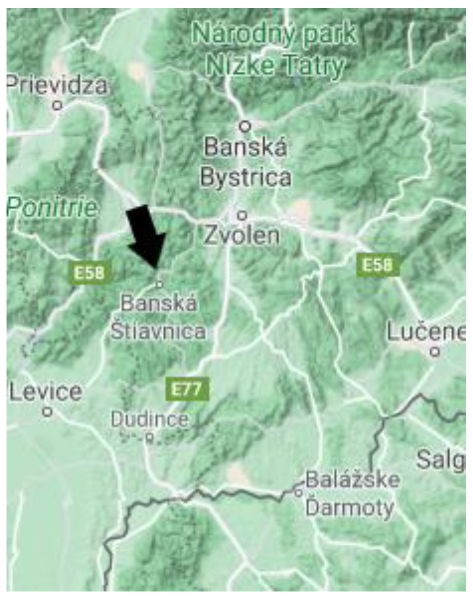
2.1. The Study Area

The article presents examples of application of the above-described theoretical basis for selected ESS assessment procedures in the area of UNESCO World Heritage site Banská Štiavnica and its surroundings. The research on the model territory was executed during 2016–2019 within the project “Ecosystem services of the landscape ecological complexes in the area of the UNESCO World Cultural and Natural Heritage site Banská Štiavnica and surrounding technical monuments” by the UNESCO-chair of the Faculty of Ecology and Environmental Studies of the Technical University in Zvolen and by the Institute of Landscape Ecology of Slovak Academy of Sciences in Bratislava.

During the research, we applied both theoretical and methodological approaches described above on two hierarchical levels—on the regional level (part of the district Banská Štiavnica) and the local level (Ilijský creek watershed and Žakýľ village). The model area is located in the Central Slovakian neo-volcanic mountain named Štiavnické vrchy, in the range of 450 to 1015 m a.s.l. The most characteristic feature of the area is the thousand-year-old impact of the mining activities since the Bronze Age, which has created an outstanding, extraordinary diverse landscape according to all the natural features, human-influenced land cover, and man-made historical objects. All this predestined that the whole region was declared in September 1979 as Štiavnické vrchy Protected Landscape Area, and in December 1993 was listed on the UNESCO World Heritage List under the name “The town Banská Štiavnica and technical monuments in its surroundings”.

The exact description of decisive features of the study areas needed for the ESS evaluation is given by the systematic database described below.

The localisation of the study in Central Slovakia is on the sketch below (Figure 1).

2.2. The Methods

The methods used in this article have been developed by authors at the Institute of Landscape Ecology of the Slovak Academy of Sciences and in the UNESCO-Chair for Sustainable Development of the Faculty of Ecology and Environmental Sciences of Technical University in Zvolen during decades of scientific works. The methods stem from the broadly conceived methodical circle of landscape ecological planning and the methods of projecting the territorial system of ecological stability [13,52]. This methodical circle has a permanent leading line containing landscape-ecological analyses → syntheses → interpretations → evaluations → propositions, within these using several continually innovated partial methods. The base principles of the above-mentioned methods are:

−

the theory and concept of the landscape as a geosystem [9,11,12,14,46,48]. In the following text, the terms “landscape” and “geosystem” may alternate according to the context.

−

an integrated geosystem approach, which considers the landscape-ecological complexes as operational units for ESS, including the abiotic base of ecosystems.

This approach allowed us to in concrete cases apply semiquantitative or quantitative methods. The result may be marked as determination of the suitability of the landscape as geosystem for human needs from the point of view of determined ESS.

The principal methodical steps and the database arranged in GIS are for each case study the same, however, the detailed procedures are described for each case study individually (see below).

2.3. The Procedure

The procedure of ESS assessment comprised two basic steps:

−

Creating a purpose-oriented GIS database within the frame of complex spatial units—landscape-ecological complexes (LEC) and microcatchments (MCC). The concept of the database follows the geosystem approach to the landscape. Since the LECs and MCCs contain the abiotic base as well as their biotic and man-made indices, they fulfil the requirements for the real content of ecosystems. In other words: each LEC and MCC is the bearer of certain ecosystem.

−

Evaluation of selected utilitarian values of LECs and microcatchments MCC.

2.3.1. The Database—the Properties of LECs and Microcatchments MCC as Spatial Operational Units for the ESS Evaluation

The analytical and synthetized data on the geosystem are expressed as properties of LECs and MCCs. LEC and MCC serve as a comprehensive spatial object-attribute database for interpretation of whatever utilitarian values of the landscape, including ESS. Furthermore, they represent boundaries of areas for optimal utilization of the landscape. So, they have been considered as the operational units for ESS evaluation.

Each LEC and MCC is the bearer of functioning ecosystems, and, as such, is also the potential ESS provider, no matter whether we evaluate, appreciate, or utilize these ESS or not [53].

LEC have homogenic set of values of indices within its area, i.e., the value of each property of complex element is the same throughout the whole particular area of LEC [48]. Two partial complexes usually represent LEC:

−

abiocomplex (ABC) with its properties (x_i) and

−

the complex of secondary/current landscape structure (CLS), which is actually the land cover and its biotic content with its properties (y_i).

The system definition of LEC types on the model area is as follows:

LEC [ABC {x₁, x₂, x₃, x₄, x₅, x₆, x₇, x₈, x₉, x₁₀, x₁₁, x₁₂}, CLS {y₁}];

where

For ABC: x₁—geological subsoil and soil substrate; x₂—hydrogeological types of sediments and rocks; x₃—soil subtype; x₄—soil texture (grain size); x₅—soil depth; x₆—soil skeletality; x₇—slope inclination; x₈—insolation; x₉—horizontal curvature of relief; x₁₀—normal curvature of relief; x₁₁—morphographic-positional type of relief; x₁₂—average altitude a.s.l.;

For CLS: y₁—land cover units, including its vegetation content.

Microcatchments MCCs are choric landscape units delineated according the horizontal relations, basically according to the:

−

direction of the movement of the water and material on the relief, and,

−

the shape of MCCs and their mode of connection to each other in a hierarchical order. The content of MCCs is created by topical LECs. The MCC can be characterised by typological characteristics {w_i} as well as by their spatial links {z_i}.

The determination of characteristics of MCC on the model area is as follows:

MCC [{z₁, z₂, z₃, z₄, z₅}, {w₁, w₂, w₃, w₄}]

where: z₁ to z₅—the hierarchical order of microcatchments from first to fifth order, w₁—shape of microcatchments, w₂—runoff profile character, w₃—microcatchments order, w₄—belonging of the microcatchments to a higher order.

Then, the complex landscape-ecological choric-topic units can be formally described as:

MCC({z_i, w_i,}, [LEC (ABC {x_i}, CLS {y_i})])

The decisive functional aspects of LEC and MCC for ESS evaluation are as follows:

−

Each LEC and MCC have precisely defined set of properties and their values as well as precisely determined delineation of its area in the space.

−

Each LEC has a certain degree of its suitability for various human needs. Such suitability can be interpreted as their offer of ESS.

2.3.2. The Purpose-Oriented Evaluation of Properties of LEC and MCC for ESS in Model Territories

The evaluation of ESS in model territories started with the determination of the utilitarian functions of LEC and the definition of the basic presumption of the relation of LEC to determined ESS, as follows.

In the region of Banská Štiavnica:

(a)

Potential of the landscape for surface water retention in LECs (further marked as ESS WAR).

Basic presumption: the lower is the runoff in LECs, the higher is the water retention ability of landscape and the impact on microclimate regulation is more favourable, thus, the higher is the value of the ESS.

(b)

Potential for subsurface water accumulation (ESS WAC)

Basic presumption: the lower the value of runoff of a certain LEC, the higher is the possibility of infiltration into the rock, and, at the same time, the higher is the hydrogeological index of rocks, the higher is the LEC ability to accumulate the water, and the higher is the value of the ESS.

In Ilíja creek watershed:

(c)

Potential of the landscape for surface water retention in microcatchments MCCs (ESS WMC).

Basic presumption: the same as in case (a), but the object of assessment are microcatchments MCC.

(d)

Agricultural crop production (ESS ACP)

Basic presumption: the more suitable the relief and soil-ecological conditions in LECs for agricultural crop are, the higher is the value of ESS ACP.

(e)

Landscape-ecological stability (ESS LES) of microcatchments MCCs

Basic presumption: The higher the coefficient of the ecological stability of landscape-ecological complexes LECs in microcatchments MCCs is, the better the ecological stability and biological balance being offered by ecosystems is and the higher the value of ESS LES is.

(f)

Environmental quality for recreation and human health (ESS REH)

Basic presumption: The higher the heterogeneity of LECs and vegetation cover in microcatchments MCCs is, the more attractive is the microcatchments for recreation and the higher is the value of ESS ERH.

In Žakýľ village:

(g)

Potential for biomass production (ESS BMP).

Basic presumption: The more suitable the soil-ecological conditions of LECs for biota are and the more productive the vegetation units in LECs are, the higher the value of the ESS BMP is.

The above-described basic presumptions serve for selected examples as simply starting points for the selection of input indices, for their syntheses and interpretations. However, the processes of assessment are quite complex.

As examples for the detailed process, the article presents the assessment of following ESS in model territory: ACP, LES, REH, BMP (abbreviations from

Table 1. Base information on ecosystem services (ESS) evaluations.

Chosen ESS for Evaluation	Method	ESS Target Value	The Object of Assessment ESS Function	Output Determinant
WAR: Water retention in LEC and microclimate regulation	Quantitative (calculation)	Contribution of LEC to water retention in landscape and to the microclimate regulation	LEC (ABC {xi},CLS {yi})] WAR = f(LEC (ABC {xi}, CLS {yi})	Relative differences of surface runoff in LEC
WAC: Subsurface water accumulation	Combined: quantitative/semiquantitave	Contribution of LEC to water accumulation in rock environment	LEC (ABC {xi}, CLS {yi})] WAC = f(LEC (ABC {xi}, CLS {yi})	Relative differences of subsurface water accumulation
WMC: Water retention of LECs in MCCs	Quantitative (calculation)	Contribution of LEC to water retention in microcatchments MCC	MCC({zi, wi,}, [LEC (ABC {xi}), CLS {yi}]) WMC = (MCC({zi, wi,}, [LEC (ABC {xi}), CLS {yi}])	Relative differences of surface runoff in MCC
ACP: Agricultural crop production	Combined: quantitative/semiquantitave	Ability of LECs to offer conditions for arable land and fodder production	LEC (ABC {xi}, CLS {yi}) ACP = f(ABC {xi}, CLS {yi})	Suitability/limits of LEC for arable land and fodder production
LES: Landscape ecological stability	Quantitative	Contribution of LECs in MCCs to ecological stability of landscape, to biological and landscape balance in microcatchments	MCC({zi, wi,}, [LEC (ABC {xi}), CLS {yi}]) LES = f(Kes MCC)	Coefficient of ecological quality of microcatchments Kes MCC
REH: Environmental quality for recreation and human health	Quantitative	Contribution of LECs in MCCs to atractivity of landscape for recreation in countryside based on the evaluation of landscape heterogeneity	MCC [CLS {yi})] ERH = f(HCLSMCC, kCLS)	Entropy degree HCLS according to secondary/current landscape structure
BMP: Potential for biomass production	Semiquantitave	Ability LECs of both agricultural and forest ecosystems to offer conditions for biomass production	LEC (ABC {xi}, CLS {yi}) BMP = f(ABC {xi}, CLS {yi})	Relative differences of LEC for biomass production

). The assessment of the ESS related to water (WAR, WAC, WMC)—because of their complexity and extent—will be presented in another article.

3. Results

3.1. Agricultural Crop Production (ESS ACP)

This ESS was assessed in the area of Ilija village, near to Banská Štiavnica UNESCO World Heritage site.

The object of assessment: LEC (ABC {x_i}, CLS {y_i})

The formal functionality: ACP = f(ABC {x_i}, CLS {y_i})

The basic presumption for ESS ACP was: the more suitable the georelief and soil-ecological conditions in LECs for agricultural crops production are, the higher is the value of ESS ACP.

Brief description:

Good conditions for agricultural production primarily depends on the production potentials of soil-ecological conditions that determine the natural biomass production. The production potential then significantly influences the modes and priorities of agricultural practice. Of course, the concrete way of land-use depends also on regional differences of socio-economic conditions, market possibilities, etc.

In the model territory, we focused exclusively on LEC´s production potential for agricultural crop given by the properties of primary structure of landscape, in particular the properties of soil and georelief.

The process of the ESS ACP assessment was as follows:

(a)

Determination of ESS ACP based on the selected properties of abiocomplexes ABC.

The decisive criteria for ESS ACP are the physical properties of geological substrate, quaternary sediments, soil, and georelief, namely:

• Availability of field’s av: the conditions for machinery entrance to the fields taking into account the stability of movement of cultivation mechanisms. The availability has been defined according to slope angle (x₇) and morphographic-positional type of relief (x₁₁) (see the definition of database in Section 2.3.1). The function is simple:

  av = f (x₇; x₁₁),

  and can be characterised as: the bigger the inclination of the slope is, the worse is the availability; the higher the field is located, the worse is the availability.
• Cultivability of the soils cv: the possibility of ploughing and other agro-technical activities. The cultivability can be characterised as the function of analytical indicators, x₁—substrate, x₄—soil grain size, x₅—soil depth, x₆—soil skeletality, x₇—slope angle, i.e.

  cv = f (x₁, x₄, x₅, x₆, x₇).

The function can be characterised as:

−

the more gravel and rock elements there are in the soil substrate, the bigger is soil skeletality and the smaller is the soil depth and the worse is the cultivability;

−

the finer the soil grain size is, the more difficult the soil disconnectability. In that case, the soil waterlogging is higher; soil permeability is getting worse, and, subsequently, the possibility for tillage is getting worse;

−

the higher the slope inclination is, the worse is the cultivability.

Other indicators influencing the ESS ACP have lower impact on the differentiation of conditions for cultivation.

The suitable way of determination of final values of ESS ACP is the determination of different levels of reduction of cultivability. Different numbers and colours indicate the level of reduction in

Table 2. The values of the abiocomplexes (ABC) for ESS agricultural crop production (ACP) according to the cultivability.

Soil Grain Size →	Light	Light	Light	Medium Heavy	Medium Heavy	Medium Heavy	Light	Heavy	Medium Heavy	Heavy	Heavy	Very Heavy	Very Heavy	Light	Very Heavy	Medium Heavy	Heavy	Clay	Clay	Light	Medium Heavy	Heavy	Very Heavy	Clay	Clay	Clay
Slope → Skeleton, depth ↓	≤1°	1°−3°	3°−7°	≤1°	1°−3°	3°−7°	7°−12°	≤1°	7°−12°	1°−3°	3°−7°	≤3°	3°−7°	12°−17°	7°−12°	12°−17°	7°–12°	≤3°	1°−3°	17°−25°	17°−25°	17°−25°	12°−25°	3°−7°	7°−12°	17°−25°
Without skelet, deep	100	97.1	89.0	80.7	76.9	76.0	65.3	62.6	57.9	47.5	35.6	32.6	29.7	25.2	17.8	5.9	5.9	3.5	2.0	0.0	0.0	0.0	0.0	0.0	0.0	0.0
	1	1	1	2	2	3	3	4	4	5	6	7	7	8	8	9	9	10	10	0	0	0	0	0	0	0
Without skelet, medium deep	89.9	87.2	81.9	79.6	72.2	68.7	68.3	57.7	56.0	51.2	42.0	30.8	28.2	26.7	21.8	15.9	5.3	3.9	3.7	0.0	0.0	0.0	0.0	0.0	0.0	0.0
	2	2	2	3	3	4	4	5	5	5	6	7	8	8	8	9	9	10	10	0	0	0	0	0	0	0
Medium skelet, medium deep	69.0	66.9	62.9	60.2	54.5	51.9	52.5	42.2	42.3	37.4	30.7	20.9	19.2	20.5	14.8	12.8	5.8	2.8	2.1	0.0	0.0	0.0	0.0	0.0	0.0	0.0
	4	4	4	4	5	5	5	6	6	7	7	8	8	9	9	9	9	10	10	0	0	0	0	0	0	0
Medium skelet, shallow	56.7	55.0	51.6	48.7	44.1	42.0	43.1	33.0	34.2	29.3	24.0	15.9	14.8	13.8	10.7	9.7	3.0	1.5	1.2	0.0	0.0	0.0	0.0	0.0	0.0	0.0
	5	5	5	6	6	6	6	7	7	8	8	8	9	9	9	9	10	10	10	0	0	0	0	0	0	0
Heavy skelet, shallow	41.5	40.2	37.8	31.2	31.2	29.8	31.3	21.7	24.2	19.2	15.8	7.9	7.2	12.3	5.6	4.9	2.0	0.0	0.0.	0.0	0.0	0.0	0.0	0.0	0.0	0.0
	6	6	7	7	7	8	7	8	8	9	9	9	9	9	9	10	10	0	0	0	0	0	0	0	0	0
Heavy skelet, without soil	0.0	0.0	0.0	0.0	0.0	0.0	0.0	0.0	0.0	0.0	0.0	0.0	0.0	0.0	0.0	0.0	0.0	0.0	0.0	0.0	0.0	0.0	0.0	0.0	0.0	0.0
	0	0	0	0	0	0	0	0	0	0	0	0	0	0	0	0	0	0	0	0	0	0	0	0	0	0

The values in the upper part of the squares mean the suitability of given ABC for cultivability in % in comparison to the best cultivability. The numbers 1 to 10 mean the values (rank) for ESS ACP: 1–7—suitable for ESS ACP, 8—limited ESS ACP, 9—restricted ESS ACP, 10 and 0—excluded ESS AC.

, as: without colours—preferred and possible conditions for ESS ACP ranked from 1 to 7 (1—best conditions, 7—weakest conditions but still not limited), yellow (rank 8)—limited, orange (rank 9)—restricted, red (rank 10)—excluded conditions for ESS ACP (Table 2).

The results are expressed in the Table 2.

(b)

Determination of ESS ACP based on the selected properties of secondary/current landscape structure CLSs.

The above-determined values of ESS ACP according to ABC properties are valid only for the agricultural land. The land use—the elements of the secondary/current landscape structure CLSs—is definitely a strong limitation for ESS ACP. The limitation of the ESS ACP according to the CLSs is quite simply: the land use forms as built-up areas, forests, greenery, water areas, means a definite limitation for production on arable land. These limits could be changed by radical change of land use, but for actual ESS ACP these areas are excluded.

(c)

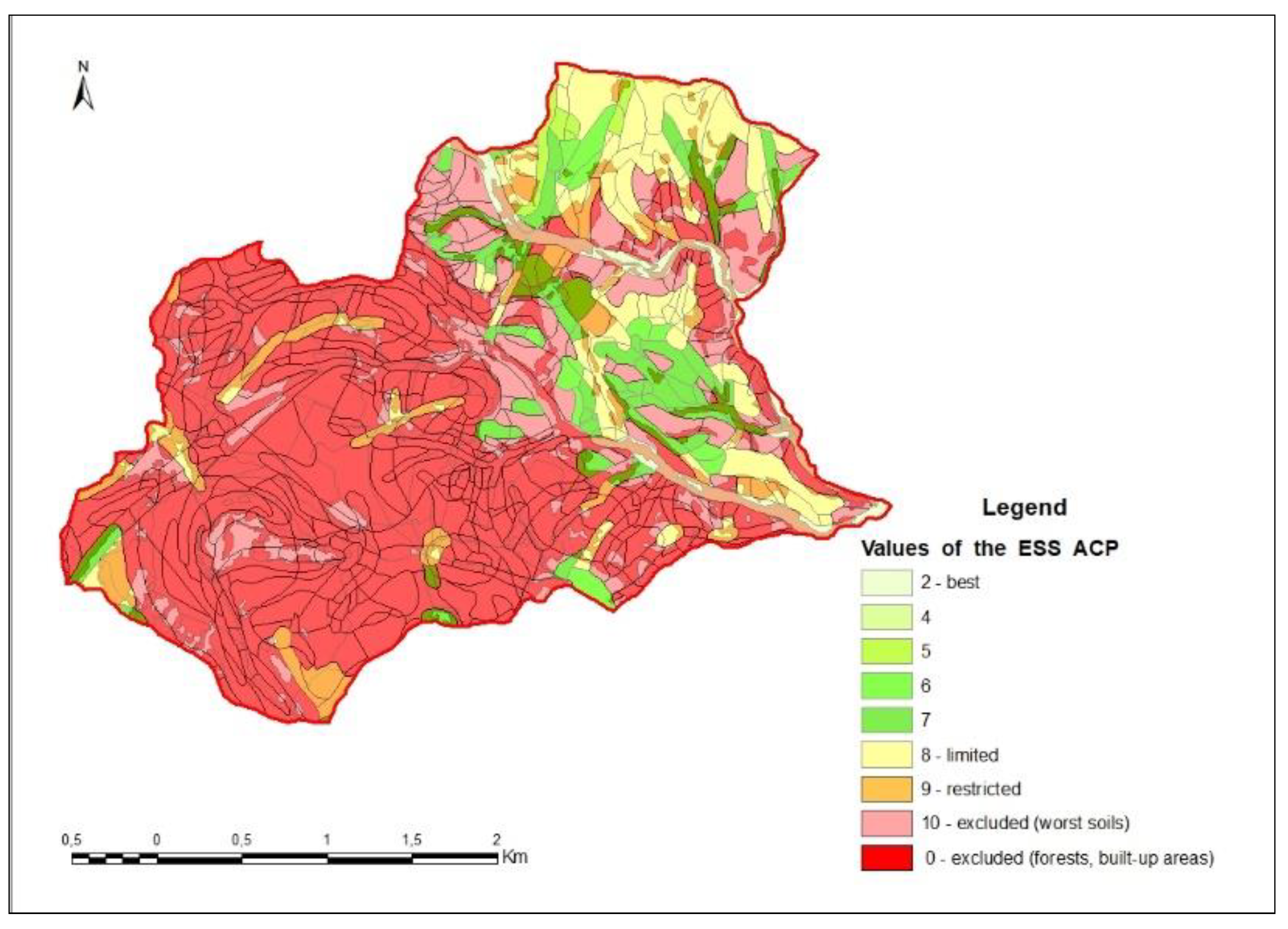
Expression of ESS ACP on the map.

The above-defined values of ESS ACP based on availability, cultivability, and present land use can be expressed on the maps where the base spatial units are areas of LECs. The characteristics of the values of ESS ACP are as follows:

−

LECs with positive values of the ESS ACP in different degree (LECs suitable for agricultural production, ranked from 1 to 7 in Table 2, where 1 = highest value);

−

LECs with limited values for ESS ACP (limited for agricultural production, rank 8);

−

LECs with restricted values for ESS ACP (restricted for agricultural production, rank 9);

−

LECs with zero values for ESS ACP (excluded for agricultural production because of worst soil and relief condition, rank 10);

−

LECs with zero values for ESS ACP (excluded for agricultural production because of current land-use—forests and built-up areas, rank 0).

The spatial distribution of these values is presented in Figure 2.

It is to be added, that the definition of the ESS ACP was not the final goal of this research. This result was the base for the further steps of the project “Ecosystem services of the landscape ecological complexes in the area of the UNESCO World Cultural and Natural Heritage site Banská Štiavnica and surrounding technical monuments”. The ESS was an important argument for the proposal of the ecologically optimum changes of land-use in (Figure 3).

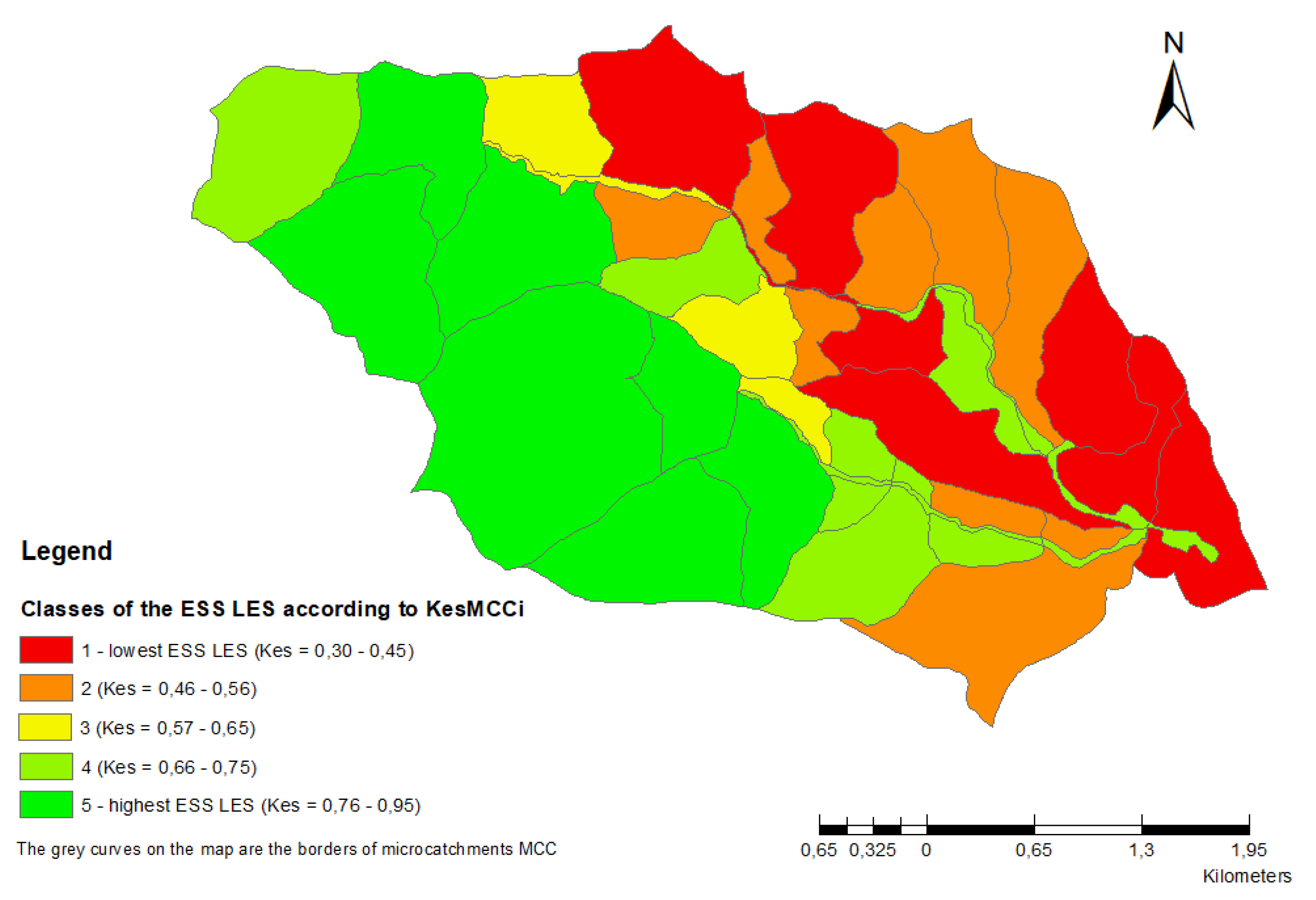
3.2. Landscape-Ecological Stability (ESS LES) of Microcatchments (MCCs)

This ESS was assessed in the watershed of Ilijský potok creek in the Štiavnické vrchy mountain.

The object of assessment: MCC_i ({z_i, w_i,}, [LEC (ABC {x_i}, CLS {y_i})])

The formal functionality: LES = f(K_es ^MCCi)

The basic presumption for the ESS LES was as follows: The higher the coefficient of the ecological stability is of individual elements of the secondary/current landscape structure CLS and of landscape-ecological complexes LECs in microcatchments MCCs, the better is the ecological stability and biological balance being offered by ecosystems and the higher is the value of ESS LES.

Brief description:

For the purposes of this ESS assessment, the decisive index is the contribution of particular microcatchments to the overall ecological stability and balance of the whole watershed, while the individual microcatchments have very different structure of landscape-ecological complexes LEC.

According to [54], the spatial stability of the landscape can be characterised as follows: the landscape is composed of elements with various internal stability, including the unstable ones. However, in general, it can be stable due to the spatial effect of stable elements. Following this consideration, the spatial ecological stability of the landscape can be determined as the dynamic ability of the landscape structure to maintain both the vertical and horizontal ecological relations within ecosystems and among ecosystems at required (model) level. This can be applied also in the case when the landscape is composed by ecosystems of a different ecological stability degree [13,55]. So, the higher the proportion of ecologically stable elements is, the higher is the landscape ecological stability of the whole landscape [49] and the higher is the ability of the landscape to provide biological-ecological functions as well as many other utilitarian functions.

According to these theoretical starting points, the determination of the ESS LES had following steps:

(a)

The determination of coefficient of ecological stability of the individual elements of the secondary/current landscape structure CLS—k_CLSi.

The differentiation of k_CLSivalues (

Table 3. Coefficient of ecological stability of the elements of secondary/current landscape structure.

i	CLSi Elements	kCLSi
1	Deciduous forest	1
2	Mixed forest dominated by deciduous trees	0.95
3	Mixed forest with balanced composition	0.9
4	Mixed forest dominated by conifers	0.85
5	Coniferous forest	0.75
6	Continuous shrub cover, small woods	0.7
7	Grassland with shrubs	0.7
8	Water areas, wetlands, peatlands	0.65
9	Meadows and pastures	0.65
10	Orchards, vineyards	0.5
11	Urban greenery	0.4
12	Arable land	0.25
13	Sport (leisure) areas	0.25
14	Rocks, terrain notches	0.2
15	Other urban areas, courts	0.1
16	Buildings and other technical elements	0.0
17	Waste sites	0.0
18	Transport objects, roads, parking places	0.0

) reflects the long-term experience of many authors resulting from their biological-ecological researches [13,27,30,42,56]. The values of k_CLSi mirror the intrinsic biological-ecological values of the elements of CLSs, as well as their abilities to provide utilitarian functions. According these researches, we determined the following values of k_CLSi:

Considering that an element provides positive influence on overall ecological stability according to its intrinsic values expressed by k_CLSi and according to its spatial extent, we can calculate the relative proportion of ecologically stable areas in each microcatchments as a sum of areas of individual elements of CLS_i weighted by their k_CLSi in microcatchments MCC according to the formula:

P_kes^MCCi = ∑ΔCLS_i × k_CLSi.

where

P_kes^MCCi—the ecologically stable area of microcatchments MCC_i;

ΔCLS_i—the area of each individual element of CLS_i in the MCC_i;

k_CLSi—coefficient of the ecological stability of the elements of CLS_i.

The value of P_kes^MCCi is always lower than the total sum of the areas of p_i.

For the comparison of the ecological quality of different MCCs it is desirable to calculate the coefficient of the ecological stability of the each particular MCCs following the formula:

K_es^MCCi = P_kes^MCCi × P^MCC−1 = (∑ ΔCLS_i × k_CLSi) × P^MCC−1

where

K_es^MCCi—coefficient of the ecological quality of the particular MCCs;

P^MCCi—total area of the microcatchments MCCs under the evaluation.

Both values, i.e. the P_kes^MCCi and the K_es^MCCi express the intrinsic ecological quality of each MCCs, as well as the contribution of individual MCCs to the overall ecological stability and balance in the study area.

(b)

Expression of the ESS LES on the map

The result of this assessment is illustrated in on map, which displays the ecological quality of individual MCCs and the contribution of microcatchments MCCs to the overall ecological stability and biological balance in the study area (Figure 4). The higher the value of K_es^MCCi, is, the higher is the ability of the MCCs to provide ESS LES. In the concrete case, the highest values of ESS LES are in MCCs with high proportion of broadleaf forests, the lowest MCCs with intensive agricultural production.

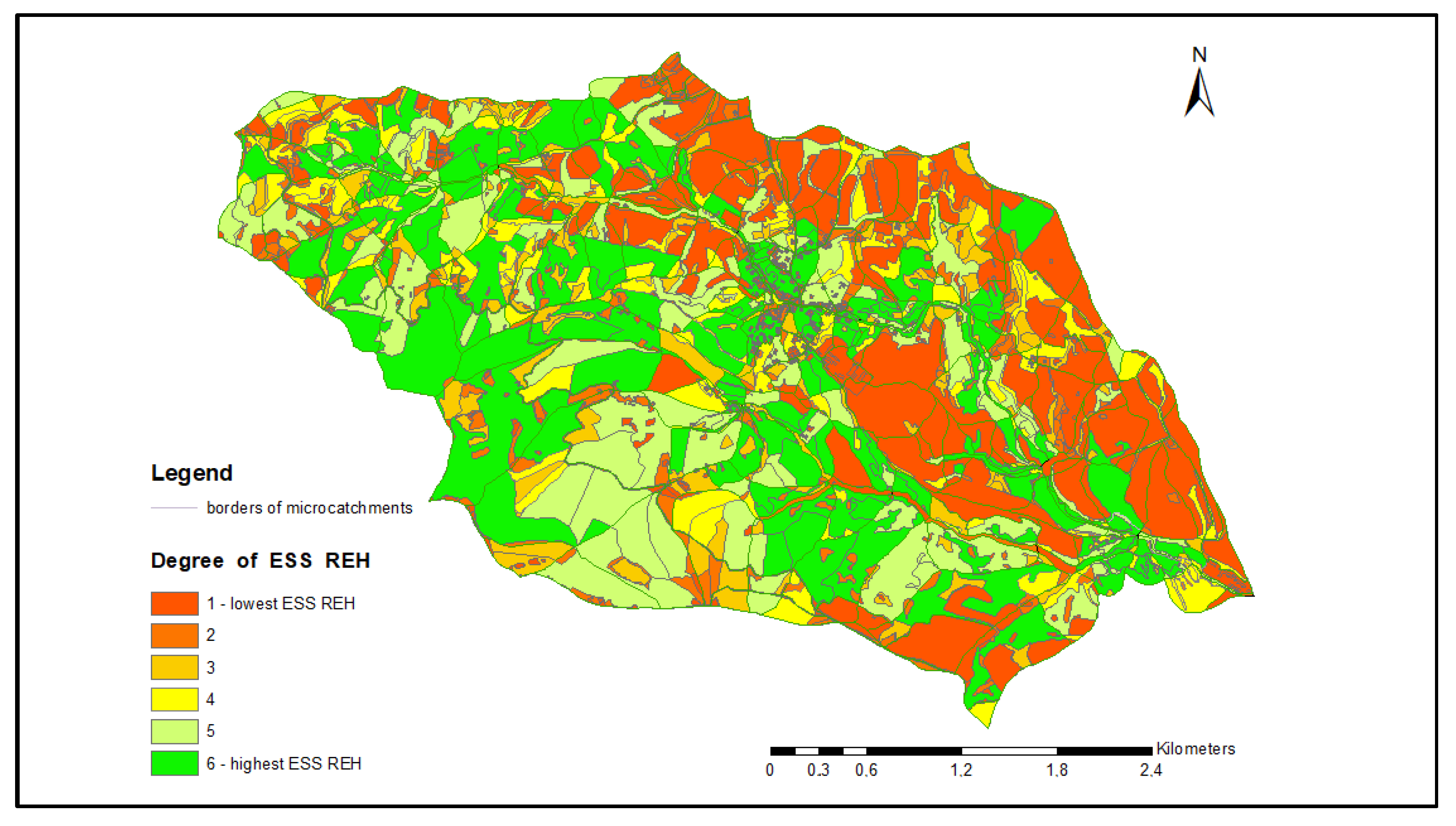
3.3. Environmental Quality of the Landscape for Recreation and Human Health (ESS REH)

This ESS was assessed in the watershed of Ilijský potok creek in the Štiavnické vrchy mountain range.

The object of assessment: MCC [CLS {y_i})]

The formal functionality: ERH = f(H_CLS^MCC, k_CLS)

Basic presumption: The higher the heterogeneity of LECs and vegetation cover in microcatchments MCCs is, the more attractive is the microcatchments for recreation and the higher is the value of ESS ERH.

Brief description:

According to the original simplified in physics, the entropy is defined as a degree of disorder, disorganisation. In the spatial context of the landscape, the entropy can be interpreted similarly: the higher the entropy is, the bigger is the disorganisation of the elements of the landscape, and the bigger is the diversity of spatial distribution of land-use elements of the evaluated area. In other words: the smaller the areas are in the study area, the bigger is the disorganisation and as such the bigger is the landscape diversity.

So, the degree of the spatial entropy can be generally considered as a degree of spatial landscape diversity.

For the purposes of the ESS REH assessment—which is itself a subjective category—we started from the precondition that the more diversified the structure of the land-use of the study area and its natural parts is —the microcatchments MCCs—the more attractive it is for the countryside tourism and recreation, and the higher is their offer to provide ESS REH.

According to these theoretical starting points, the determination of the ESS LES had the following steps:

(a)

The evaluation of the diversity of the landscape—the overall entropy of microcatchments MCCs.

The key questions for the calculation of the spatial entropy is the determination of:

−

the area to be assessed—in our case the areas of the microcatchments MCCs, and,

−

the individual elements creating the inner structure of the assessed area—in our case, the areas of the elements of the secondary/current landscape structure CLS, i.e., the land use elements.

The evaluation of the entropy of the spatial structure of the landscape is than based on the “classical” Shannon formula as follows:

$${\mathit{H}}_{\mathit{M}\mathit{C}\mathit{C}\mathit{i}}\mathit{=}{\displaystyle \mathit{\sum }}_{\mathit{i}\mathit{=}1}^{\mathit{n}}\mathit{-}\mathit{\left(}{\mathit{p}}_{\mathit{i}}\mathit{\times }\mathit{ }\mathit{l}\mathit{o}{\mathit{g}}_2{\mathit{p}}_{\mathit{i}}\mathit{\right)}$$

where:

• p_i—probability of occurrence of the individual areas of secondary/current landscape structure CLSi within the area of microcatchments, calculated as:

  $${\mathit{p}}_{\mathit{i}}\mathit{=}\frac{\mathit{\Delta }\mathit{C}\mathit{L}{\mathit{S}}_{\mathit{i}}}{{\mathit{P}}_{\mathit{M}\mathit{C}\mathit{C}\mathit{i}}}$$
• ΔCLS_i—the area size of CLS_i;
• P_MCCi—the overall area size of the evaluated microcatchments.

The result is the value of the entropy of each MCCi, caused by all elements of CLS defined in Table 3.

(b)

The evaluation of the diversity of the MCCs caused by P_MCCi “green elements”of CLS.

For the purposes of ESS REH, this base calculation can be refined. A more suitable indicator than the entropy caused by all element of the CLS (see Table 3 in Section 3.2) can be the diversity caused by chosen elements of the CLS, namely by CLSi 1 to 8 in Table 3 (“green elements”). These elements have a high degree of ecological quality, therefore, their diversity might provide higher ESS REH than the others.

In this case, the input element to the formula has been changed as follows:

$${\mathit{p}}_{\mathit{i}\mathit{g}}\mathit{=}\frac{\mathit{\Delta }\mathit{C}\mathit{L}{\mathit{S}}_{\mathit{g}\mathit{i}}}{{\mathit{P}}_{\mathit{M}\mathit{C}\mathit{C}\mathit{i}}}$$

where ΔCLS_gi means the area size of “green” elements. Then, the basic formula is modified as:

$${\mathit{H}}_{\mathit{M}\mathit{C}\mathit{C}\mathit{g}}\mathit{=}{\displaystyle \mathit{\sum }}_{\mathit{i}\mathit{=}1}^{\mathit{n}}\mathit{-}\mathit{\left(}{\mathit{p}}_{\mathit{i}\mathit{g}}\mathit{\times }\mathit{l}\mathit{o}{\mathit{g}}_2{\mathit{p}}_{\mathit{i}\mathit{g}}\mathit{\right)}$$

The situation when the microcatchments MCC have high value of entropy, i.e., high diversity, high fragmentation caused by green elements CLSg is being considered as a good state of the landscape.

(c)

Expression of the ESS REH on the map.

The result of this assessment is illustrated in Figure 5. This map expresses the ability of the microcatchments MCCs to provide ESS REH based on the spatial diversity of the green elements of CLS in MCCs, related to the maximum possible diversity of MCC in the study area.

The higher is the rate number, the higher is the diversity of the MCC and the higher is the assessed ability of the MCC to provide ESS REH.

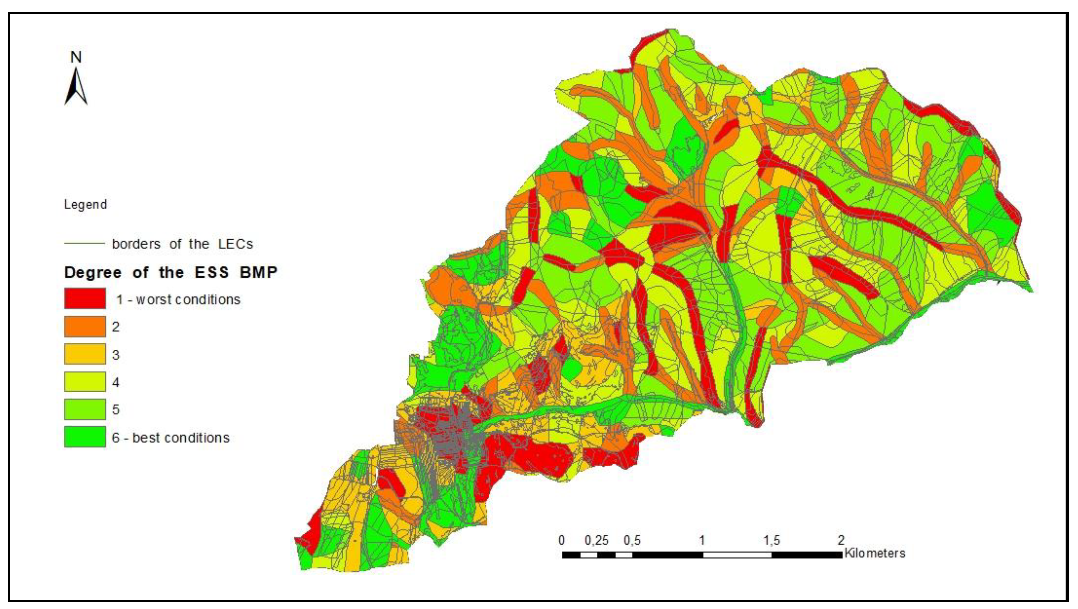
3.4. Potential for Biomass Production (ESS BMP)

The ESS BMP was assessed in the area of the Žakýľ village, near to Banská Štiavnica World Heritage site.

The object of assessment: LEC (ABC {x_i}, CLS {y_i})

The formal functionality: ESS BMP = f(ABC {x_i}, CLS {y_i})

The basic presumption for this ESS was as follows: the more suitable the abiotic conditions of the landscape ecological complexes LECs for biota are, and the more productive the vegetation units in LECs are, the higher the value is of the ESS BMP.

Brief description:

The abiotic conditions (soil properties, geological substrate, relief, water, and climate) expressed in abiotic complexes ABC (see Section 2.1) have decisive influence on the biomass production. In the study area, the variability of these conditions is caused mostly by the properties of the soils and georelief, since the geological, hydrological as well as climate conditions do not differentiate this area significantly.

Production potential of ABC is a decisive condition also for land use. The present land use—i.e., the elements of the secondary/current landscape structure CLS—are characterized by physiognomic-ecological formations of the land cover and by the biological-ecological quality of the real vegetation.

The conditions expressed by ABC and by CLS determine the real biomass production of each landscape-ecological complex LEC. Remember: LEC = [ABC {xi}, CLS {y₁}].

In this study area, we assessed the production potential of both agricultural and forest LECs.

According to these theoretical starting points, the determination of the ESS LES had following steps:

(a)

Evaluation of the abiotic conditions for ESS BMP.

The most important abiotic conditions for bioproduction potential expressed in abiotic complexes ABC are as follows:

−

physical-mechanical soil properties: soil depths, soil skeletality, soil grain size. Soil depths and skeletality can predetermine the volume and availability of soil mass for biota development. Soil grain size makes an impact mainly on water supply and on water permeability, sorption complex, and erosion resistance;

−

physic-chemical and physiological soil properties: soil salt regime, soil water regime determined by the soil subtype, soil reaction, the volume of nutrients and humus. These factors predetermine mainly trophic conditions, the intensity of physiological processes, therefore, the biomass growth;

−

morphometric relief conditions: inclination, normal, and horizontal curvature, relief aspect (orientation towards the cardinal points). These factors predetermine the dynamics of movement of water, materials, and energy on the surface, i.e., the volume of eroded and accumulated material, the volume of runoff, the speed of runoff, insolation. Therefore, the relief influences comprehensively the physic-mechanical and physiologic-trophic conditions of biomass production.

Of the above-mentioned indicators, the highest differentiation in the study has been observed on morphometric relief conditions, soil depth and skeletality, and soil grain size. That means that the differentiation of ESS BMP in the area is caused also by these conditions, the others display more or less equal values overall in the study area. Then, the base function, the values of these cardinal indicators can be determined as follows:

−

soil depth and skeletality: the deeper the soils and the less skelet content in the soils, the higher is the production due to the fact that there is more soil mass, and nutrients and humidity are at the disposal for biomass growth;

−

soil grain size: medium heavy loamy soils are the most favourable ones for bioproduction. They have the best water retention regime, they are the most resistant against erosion, and they have the best absorption ability. Other soil textures, as the sandy or clay soils have worse values.

−

Relief inclination: it determines the intensity, velocity, and the volume of the run-off and the material movement on the surface. Obviously, on the less sloped relief there is deeper soil, lower erosion, better supply by water and nutrients; consequently there are better conditions for bioproduction.

All these principles have been applied on each individual ABC. The results are the same, as for the ESS ACP expressed in Table 2. The ranks 1 to 10 plus 0 expressed in the Table 2 can be read here as the degree of the bioproduction potential of the abiocomplexes (ABC).

(b)

Evaluation of the biotic complex within the elements of secondary/current landscape structure CLS.

The most productive plant and animal communities have been evolved in the best above-described abiotic conditions. At the same time, humans have also utilised these areas for intensive bioproduction, where the abiotic conditions offer high productivity (as exception there are highly productive wetlands and water ecosystems that are not available for agriculture). Accordingly, we can express the relation that the high bioproduction potential of ABC attracted in the past also highly productive biotic systems—agroecosystems on arable land, where the production was supported also by intensive human impact. Nevertheless, after the humans abandoned the arable land—which is a common case in our study area—the productive agroecosystems on former arable land became less productive in comparison with forests and other ecosystems.

Accordingly, in the Žakýl village study area we applied a compromise evaluation of bioproductivity of the biotic elements of the CLS by the confrontation between land use and real productivity of biotic elements in both forest and non-forest areas. The result of this evaluation is showed in

Table 4. Coefficients of bioproductivity of the elements of CLS.

i	Elements of the CLS in Žakýľ Village Area	kBMP
1	Forests more than 120 year old	1
2	Forests 101–120 years	1
3	Forests 81–100 years	0.9
4	Forests 61–80 years	0.8
5	Forests 41–60 years	0.7
6	Forests–40 years	0.6
7	Forests 0–20 years	0.5
8	Non forest woody vegetation, shrubs	0.6
9	Grassland with non-forest woody vegetation	0.5
10	Meadows and pastures	0.4
11	Creeks	0.4
12	Arable land	0.5
13	Terrain edges, terraces	0.3
14	Cemetery and other urban greenery	0.3
15	Sport areas and playground	0.15
16	Built-up areas	0.0
17	Roads	0.0

. The relative differences between bioproductivity of the elements of CLS are expressed as coefficients k_BMP, while the highest value—k_BMP = 1, was bind to oak–hornbeam-beech forests of highest age. These forests prevail in the Žakýľ village study area. The older forests have better productivity. The value of the bioproductivity of arable land (ecosystems on arable land) in this ranking is 0.5. The values of coefficients reflect the long-term researches of the scientists in the Institute of Landscape Ecology of Slovak Academy of Sciences. They were compiled by collective expert assessment, using also other sources [13,27,30,42,55,56].

(c)

Modification of the bioproduction potential of ABC with the evaluation of the bioproductivity of the CLS elements—the ESS BMP of landscape-ecological complexes (LEC).

The compromise between the natural productivity potential of ABC and the real bioproduction of the elements of CLS is formally determined by modification of the rank of the ABC suitability for agricultural production (see Table 2) by coefficients of real biotic productivity of CLS elements k_BMP according to Table 4 on each landscape ecological complex (LEC).

The result was calculated as multiplication of the ranks of objective bioproduction potential of the abiocomplexes ABC with coefficients of bioproductivity k_BMP of the elements of CLS within LEC. Formally:

ESS BMP = ESS ACP × k_BMP

where ESS ACP are the relative values from the Table 2 (Section 3.1).

The results were after calculations ranked into six classes.

They are illustrated in Figure 6.

4. Discussion

One of the main issues for permanent discussion is the object of ESS. The presented case studies illustrated that landscape as a geosystem, actually its spatial units, expressed in a unified database in GIS as abiocomplexes (ABC), microcatchments (MCC) and elements of the secondary/current landscape structure (CLS) are suitable for assessment of very diverse ESS.

The utilitarian values of the nature, may it be marked as ESS, are without any doubt predetermined by the synergic impacts of all properties of the object of ESS. Therefore, the precondition for the correct evaluation and decision on ESS is the complexity of information. The geosystem approach allows developing a comprehensive GIS based spatial information system, which enables to interpret the same data set in very different ways (see Section 2.1). This complexity means the information on the properties on all structures of the landscape as geosystem [12,13,57].

Recognising the diversity of the character of the utility values of the ecosystems is to state the following: properties, processes, and functions of ecosystems are really and permanently existing, no matter whether we evaluate them from the point of view of social needs, or not. It is the permanent “offer” of the landscape as a complex natural resource and potential for human utilization [47,58]. On other side, humans express the “demand” for landscape resources and potentials selectively, not for all potential and not every time. The satisfaction of the demands may give to the objectively existing resources and potentials a character of “services”. The above mentioned predestines that each ESS research must determine ex ante the actual content of the given ecosystem service, namely which ESS should be concretely evaluated in the given research.

Another must is the determination of the basic presumption for the assessment of each particular ESS and their relations to decisive properties of the landscape-ecological complexes. The proper data set for each ESS assessment, concerning each particular ESS on each particular study area, are discussed in the Section 3.1 to Section 3.4

Other questions the have the character of discussion, but that are specific for each case study, are pointed in Section 3.1 to Section 3.4, in parts named “brief description” and also in the results of the case studies.

5. Conclusions

As presented in the article, the landscape as a geosystem should be considered in the light of the ESS concept as a complex/integrated natural resource for different ESS [7,32,48,59]. The landscape as a geosystem—because of its complex character—is able to fulfil different functions and different needs of the humans, including ESS.

In the presented case studies, the object of ESS assessment was the landscape as a geosystem, in particular its complex spatial units—landscape-ecological complexes—that consist of both the abiotic base and the biota. The results of the case studies are based on the assessment of these complex objects.

As also presented, the landscape-ecological approach to ESS evaluation is very comprehensive. Therefore, it is inevitable to define the character and content of assessed ESS for each concrete work based on deep knowledge of the geosystem, its elements, as well as the different role of primary, secondary/current, and tertiary landscape structure for ESS.

In the presented studies, the first step of the assessment process was the definition of the basic presumption for each particular ESS in relation to the decisive properties of the landscape-ecological complexes. This step was parallel to the creation of a comprehensive database supported by GIS technology.

The diversity of the method of ESS assessment is so big that we dare to state that actually there is no generally accepted method [3,4,35]. Taking into account this fact, as well as our long-term experiences in applied landscape ecological studies in concrete territories, in the presented case studies we applied as the basic criteria of evaluation the suitability of landscape ecological complexes for practical purposes on the base of abiocomplexes (ABC), microcatchments (MCCs), and current landscape structure CLS. The results were presented as relative suitability of the ABCs, MCCs, and CLSs for particular ecosystem services.

With regard to above statements, the main conclusion related to the results is that the geosystem approach to the ESS assessment enables more objective, more comprehensive, and more calculable values for the given ESS than just an expert evaluation of land cover elements or vegetation formations [3,4,38], since the results consist of both the abiotic base and the biotic cover of complex spatial landscape ecological units ABCs, MCCs, CLSs, and LECs.

All these problems clearly underline that in the current state of the ESS concept, each model territory needs individual specification of all the object of ESS, the content of ESS, and the methods of evaluation of ESS. Let us add that there is no inevitable necessity to name each evaluation of utility values as ecosystem services.

There are innumerable studies and surveys—also critical ones—that deal with the ESS concept and their different aspects [15,60]. Generally, it is to express an optimistic opinion that the ESS concept has an important mainstream effect, allowing the ecological ideas to enter economics and politics [15,37]. Nevertheless, just the need to interpret the ESS results in an acceptable form for policy, decision-makers, and planning authorities, must not be an excuse for avoiding the balance between scientifically correct research and its application to practical form, regardless of any trendy challenges coming from politics and economics. This aspect of problems appeared already in a number of studies [15,51,61].

Finally, it is to be underlined that in spite of whatever criticism, the concept of ESS brought a new wave of appreciation of the landscape sciences in politics, decision-making, planning, and other practices. The concept of ecosystem services surely belongs to mainstream topics regarded also by EU environmental strategies, which should be reflected also in the national environmental policies of EU member states [17,21,47,62,63,64]

References

1. Grunewald, K.; Bastian, O. (Eds.) Ecosystem Services–Concepts, Methods and Case Studies, 1st ed.; Springer: Berlin/Heidelberg, Germany, 2015; all chapters; p. 312. [Google Scholar]
2. Tansley, A.G. The use and abuse of vegetational concepts and terms. Ecology 1935, 16, 284–307. [Google Scholar] [CrossRef]
3. Dick, J.; Turkelboom, F.; Arandia, I.I.; Woods, H. Stakeholder´s perspectives on the operationalisation of the ecosystem service concept: Results from 27 case studies. Ecosyst. Serv. 2018, 29, 552–565. [Google Scholar] [CrossRef] [Green Version]
4. Saarikoski, H.; Primmer, E.; Saarela, S.R.; Antunes, P.; Aszalós, R.; Baró, F.; Berry, P.; Blanko, G.G.; Goméz-Baggethun, E.; Carvalho, L. Institutional challenges in putting ecosystem service knowledge in practice. Ecosyst. Serv. 2018, 29, 579–598. [Google Scholar] [CrossRef]
5. Burkhard, B.; Kroll, F.; Müller, F.; Windhorst, W. Landscape’s capacities to provide ecosystem services-a concept for land cover based assessments. Landsc. Online 2009, 15, 1–12. [Google Scholar] [CrossRef]
6. Haase, G. Zu Inhalt und Terminologie der topischen und chorischen Landschaftserkundung. In Proceedings of the International Symposium on Problems of Ecological Landscape Research, Smolenice, Slovakia, 28 November–1 December 1973; ÚBK SAV: Bratislava, Slovakia, 1973; p. 19. [Google Scholar]
7. Neef, E. Die Theoretischen Grundlagen der Landschaftslehre, 1st ed.; H. Haack: Gotha/Leipzig, Germany, 1967; p. 152. [Google Scholar]
8. Isachenko, A.G. Predstavlenije o geosisteme v sovremennoj fizičeskoj geografiji. Izv. VGO 1981, 113, 297–306. [Google Scholar]
9. Preobrazhenskiy, V.S. Geosystem as an Object of Landscape study. GeoJournal 1983, 7, 131–134. [Google Scholar] [CrossRef]
10. Krcho, J. Prírodná časť geosféry ako kybernetický systém a jeho vyjadrenia v mape. Geogr. Časopis 1968, 20, 115–130. [Google Scholar]
11. Demek, J. The landscape as a geosystem. Geoforum 1978, 9, 29–34. [Google Scholar] [CrossRef]
12. Miklós, L.; Izakovičová, Z. Kraj. Ako Geosystém; VEDA, SAV: Bratislava, Slovakia, 1997; p. 152. [Google Scholar]
13. Miklós, L.; Diviaková, A.; Izakovičová, Z. Ecological Networks and Territorial Systems of Ecological Stability; Springer International Publishing: Berlin/Heidelberg, Germany, 2019; p. 159. [Google Scholar]
14. Bastian, O.; Grunewald, K.; Khoroshev, A.V. The significance of geosystem and landscape concepts for the assessment of ecosystem services: Exemplified in case study in Russia. Landsc. Ecol. 2015, 30, 1145–1164. [Google Scholar] [CrossRef]
15. Abson, D.J.; von Wehrden, H.; Baumgärtner, S.; Fischer, J.; Hanspach, J.; Härdtle, W.; Heinrichs, H.; Klein, A.M.; Lang, D.J.; Martens, P. Ecosystem services as a boundary object for sustainability. Ecol. Econ. 2014, 103, 29–37. [Google Scholar] [CrossRef]
16. Haines-Young, R.; Potschin, M. Common International Classification of Ecosystem Services (CICES): Consultation on Version 4, August–December 2012. Available online: https://unstats.un.org/unsd/envaccounting/seearev/GCComments/CICES_Report.pdf (accessed on 18 November 2020).
17. MEA. Linking Ecosystem Services and Human Wellbeing; Island Press: Washington, DC, USA, 2005; p. 60. [Google Scholar]
18. Costanza, R.; d’Arge, R.; de Groot, R.; Farber, S.; Grasso, M.; Hannon, B.; Limburg, K.; Naeem, S.; O’Neill, R.V.; Paruelo, J.; et al. The Value of the World’s Ecosystem Services and Natural Capital. Nature 1997, 387, 253–260. [Google Scholar] [CrossRef]
19. Landers, D.H.; Nahlik, A.M. Final Ecosystem Goods and Services Classification System (FEGS-CS). EPA/600/R-13/ORD–004914, 1st ed.; U.S. Environmental Protection Agency, Office of Research and Development: Washington, DC, USA, 2013. [Google Scholar]
20. Fisher, B.; Turner, R.K.; Morling, P. Defining and classifying ecosystem services for decision making. Ecol. Econ. 2009, 68, 643–653. [Google Scholar] [CrossRef] [Green Version]
21. de Groot, R.S.; Alkemade, R.; Braat, L.; Hein, L.; Willemen, L. Challenges in integrating the concept of ecosystem services and values in landscape planning, management and decision making. Ecol. Complex. 2010, 7, 260–272. [Google Scholar] [CrossRef]
22. Gomez-Baggethum, E.; Barton, D. Classifying and valuing ecosystem services for urban planning. Ecol. Econ. 2013, 86, 235–245. [Google Scholar] [CrossRef]
23. Melichar, J. Ekonomické hodnocení ekosystémových služeb. Životné Prostr. 2010, 44, 78–83. [Google Scholar]
24. Ferraro, P.J. The Future of Payments for Ecosystem Services. Conserv. Biol. 2011, 25, 1134–1138. [Google Scholar] [CrossRef]
25. Grunewald, K.; Bastian, O. Development and Fundamentals of the ES approach. In Ecosystem Services–Concepts, Methods and Case Studies, 1st ed.; Grunewald, K., Bastian, O., Mansfeld, K., Eds.; Springer: Berlin/Heidelberg, Germany, 2015; Volume 1, pp. 13–34. [Google Scholar]
26. Eliáš, P. Od funkcií vegetácie k ekosystémovým službám. Životné Prostr. 2010, 44, 59–64. [Google Scholar]
27. Jurko, A. Ekologické a Socioekonomické Hodnotenie Vegetácie, 1st ed.; Príroda: Bratislava, Slovakia, 1990; p. 195. [Google Scholar]
28. Midriak, R. Ochrana pôdy a krajinno-ekologická únosnosť územia národného parku Nízke Tatry. Ochr. Prírody 1993, 12, 9–53. [Google Scholar]
29. Haada, L.; Topercer, J.; Kartusek, V.; Mederly, P. Systém ekologickej kvality krajiny-ďalší prístup k manažmentu krajiny. Životné Prostr. 1995, 29, 271–273. [Google Scholar]
30. Hrnčiarová, T.; Miklóš, L.; Kalivodová, E.; Kubíček, F.; Ružičková, H.; Izakovičová, Z.; Drdoš, J.; Rosová, V.; Kovačevičová, S.; Midriak, R. Ekologická únosnosť krajiny: Metodika a aplikácia na 3 benefičné územia. I-IV. časť. In Ekologický Projekt MŽP SR; ÚKE SAV: Bratislava, Slovakia, 1997. [Google Scholar]
31. Čaboun, V.; Tutka, J.; Moravčík, M.; Kovalčík, M.; Sarvašová, Z.; Schwarz, M.; Zemko, M. Uplatňovanie Funkcií Lesa v Krajine; Národné Lesnícke Centrum: Zvolen, Slovakia, 2010; p. 285. [Google Scholar]
32. Haase, G. Zur Ableitung und Kennzeichnung von Naturraumpotentialen. Petermanns Geogr. Mitt. 1978, 122, 113–125. [Google Scholar]
33. Tremboš, P. Potenciál krajiny, jeho hodnotenie a využitie v územno-plánovacej praxi. Životné Prostr. 1993, 27, 41–43. [Google Scholar]
34. Džatko, M.; Sobocká, J. Príručka Pre Používanie Máp Pôdno-Ekologických Jednotiek. Inovovaná Príručka Pre Bonitáciu a Hodnotenie Poľnohospodárskych Pôd Slovenska, 1st ed.; Výskumný Ústav Pôdoznalectva a Ochrany Pôdy: Bratislava, Slovakia, 2009; pp. 46–102. [Google Scholar]
35. Lamarque, P.; Que-Tier, F.; Lavorel, S. The diversity of the ecosystem services concept and its implications for their assessment and management. Comptes Rendus Biol. 2011, 334, 441–449. [Google Scholar] [CrossRef] [PubMed]
36. Albert, C.; Galler, C.; Hermes, J.; Neuendorf, F.; von Haaren, C.; Lovett, A. Applying ecosystem services indicators in landscape planning and management: The ES-in-Planning framework. Ecol. Indicat. 2015, 61, 100–113. [Google Scholar] [CrossRef]
37. Harrison, P.A.; Harmáčková, Z.V.; Aloe Karabulut, A.L.; Brotons, M.; Cantele, J.; Claudet, R.W.; Dunford, A.; Guisan, I.P.; Holman, S.; Jacobs, K.; et al. Synthesizing plausible futures for biodiversity and ecosystem services in Europe and Central Asia using scenario archetypes. Ecol. Soc. 2019, 24, 27. [Google Scholar] [CrossRef]
38. Dunford, R.; Harrison, P.; Smith, A.; Dick, J.; Barton, D.; Martín-López, B.; Kelemen, E.; Jacobs, S.; Saarikoski, H.; Turkelboom, F.; et al. Integrating methods for ecosystem service assessment: Experiences from real world situations. Ecosyst. Serv. 2018, 29, 499–514. [Google Scholar] [CrossRef]
39. Wu, J. Key concepts and research topics in landscape ecology revisited: 30 years after the Allerton Park workshop. Landscape Ecol. 2013, 28, 1–11. [Google Scholar] [CrossRef]
40. Stępniewska, M.; Lupa, P.; Mizgajski, A. Drivers of the ecosystem services approach in Poland and perception by practitioners. Ecosyst. Serv. 2018, 33, 59–67. [Google Scholar] [CrossRef]
41. Izakovičová, Z. Ecological interpretations and evaluation of encounters of interests in landscape. Ekológia 1995, 14, 261–275. [Google Scholar]
42. Papánek, F. Teória a Prax Funkčne Integrovaného Lesného Hospodárstva; Príroda: Bratislava, Slovakia, 1978; p. 218. [Google Scholar]
43. Brandt, J.; Vejre, H. (Eds.) Multifunctional Landscapes: Theory, Values and History, 1st ed.; WIT Press: Southampton, UK, 2004; Volume 1, pp. 3–32. [Google Scholar]
44. von Bertalanffy, L. General System Theory. Foundations, Development and Applications, 1st ed.; George Braziller: New York, NY, USA, 1968; pp. 30–54. [Google Scholar]
45. Sochava, V.B. Vvedenje v Učenije o Geosystemach, 1st ed.; Nauka: Novosibirsk, Russia, 1977; p. 236. [Google Scholar]
46. Frolova, M. From the Russian/Soviet landscape concept to the geosystem approach to integrative environmental studies in an international context. Landscape Ecol. 2019, 34, 1485–1502. [Google Scholar] [CrossRef]
47. Bastian, O.; Grunewald, K.; Syrbe, R.U. Space and time aspects of ecosystem services, using the example of the EU Water Framework Directive. Int. J. Biodivers. Sci. Ecosyst. Serv. Manag. 2012, 8, 5–16. [Google Scholar] [CrossRef] [Green Version]
48. Miklós, L.; Kočická, E.; Izakovičová, Z.; Kočický, D.; Špinerová, A.; Diviaková, A.; Miklósová, V. Landscape as a Geosystem; Springer International Publishing: Berlin/Heidelberg, Germany, 2019; p. 245. [Google Scholar]
49. Ružičková, H.; Ružička, M. Druhotná štruktúra krajiny ako kritérium biologickej rovnováhy. Quest. Geobiol. 1973, 12, 23–62. [Google Scholar]
50. Izakovičová, Z.; Miklós, L.; Miklósová, V. Integrative Assessment of Land Use Conflicts. Sustainability 2018, 10, 3270. [Google Scholar] [CrossRef] [Green Version]
51. von Haaren, C.; Albert, C. Integrating ecosystem services and environmental planning: Limitations and synergies. Int. J. Biodivers. Sci. Ecosyst. Serv. Manag. 2011, 7, 150–167. [Google Scholar] [CrossRef] [Green Version]
52. Ružička, M.; Miklós, L. Landscape-ekological planing (LANDEP) in the Process of the Teritorial Planning. Ekológia 1982, 1, 297–312. [Google Scholar]
53. Miklósová, V. Hodnotenie ekosystémových služieb v záujmovom území národnej prírodnej rezervácie Klátovské rameno. Ekol. Štúdie 2017, 8, 44–53. [Google Scholar]
54. Naveh, Z.; Liebermannn, A.S. Landscape Ecology-Theory and Applications, 2nd ed.; Springer: New York, NY, USA, 1993; p. 360. [Google Scholar]
55. Miklós, L. Stabilita krajiny v ekologickom genereli SSR. Životné Prostr. 1986, 20, 131–134. [Google Scholar]
56. Špulerová, J. Evaluation of vegetation and their limits for sustainable development. GeoScape Altern. Approaches Middle-Eur. Geogr. 2010, 5, 175–183. [Google Scholar]
57. Šúriová, N.; Izakovičová, Z. Territorial system of anthropogenic stress factors in landscape ecological planning. Ekológia 1995, 14, 181–189. [Google Scholar]
58. Dickson, B.; Blaney, R.; Miles, L.; Regan, E.; Soesbergen, A.; van Väänänen, E.; Blyth, S.; Harfoot, M.; Martin, C.S.; McOwen, C.; et al. Towards a Global Map of Natural Capital: Key Ecosystem Assets, 1st ed.; UNEP: Nairobi, Kenya, 2014; pp. 4–33. [Google Scholar]
59. Antrop, M. Background concepts for integrated landscape analysis. Agric. Ecosyst. Environ. 2000, 77, 17–28. [Google Scholar] [CrossRef]
60. Bordt, M.; Saner, M. A critical review of ecosystem accounting and services frameworks. One Ecosyst. 2018, 3, e29306. [Google Scholar] [CrossRef]
61. Bastian, O.; Krönert, R.; Lipský, Z. Landscape Diagnosis on Different Space and Time Scales—A Challenge for Landscape Planning. Landsc. Ecol. 2006, 21, 359–374. [Google Scholar] [CrossRef]
62. Our Life Insurance, Our Natural Capital: An EU Biodiversity Strategy to 2020; Policy Document. Communication from the Commission to the European Parliament, the Council, the Economic and Social Committee and the Committee of the Regions. COM(2011) 244 Final; European Commission: Brussels, EU, 2011; Available online: https://www.eea.europa.eu/policy-documents/our-life-insurance-our-natural (accessed on 3 December 2020).
63. Díaz, S.; Settele, J.; Brondízio, E.; Ngo, H.T.; Guèze, M.; Agard, J.; Pfa, C. (Eds.) IPBES. Summary for Policymakers of the Methodological Assessment of Scenarios and Models of Biodiversity and Ecosystem Services of the Intergovernmental Science-Policy Platform on Biodiversity and Ecosystem Services; Secretariat of the Intergovernmental Science-Policy Platform on Biodiversity and Ecosystem Services: Bonn, Germany, 2016; p. 32. [Google Scholar]
64. Maes, J.; Teller, A.; Erhard, M. Mapping and Assessment of Ecosystems and their Services: Indicators for Ecosystem Assessments under Action 5 of the EU Biodiversity Strategy to 2020; Publications office of the European Union: Luxembourg, 2014. [Google Scholar]
Figure 1. The localisation of the study area in the Central Slovakia Region.
Sustainability 12 10167 g001
Figure 2. The values of the ESS ACP in the area of Ilija village.
Sustainability 12 10167 g002
Figure 3. Proposals of changes for the ecologically optimum land-use based on limited and restricted values of ESS ACP.
Sustainability 12 10167 g003
Figure 4. The ability of microcatchments (MCCs) to provide LES ESS landscape-ecological stability.
Sustainability 12 10167 g004
Figure 5. The ability of microcatchments (MCCs) to provide ESS recreation and human health (REH) based on the spatial diversity of the landscape caused by “green elements” of secondary/current landscape structure (CLS).
Sustainability 12 10167 g005
Figure 6. The ESS biomass production (BMP) of the LEC based on the quality of ABCs and the productivity of CLSs.
Sustainability 12 10167 g006