Feature Extraction and Representation of Urban Road Networks Based on Travel Routes

Abstract

Extraction of traffic features constitutes a key research direction in traffic safety planning. In previous traffic tasks, road network features are extracted manually. In contrast, Network Representation Learning aims to automatically learn low-dimensional node representations. Enlightened by feature learning in Natural Language Processing, representation learning of urban nodes is studied as a supervised task in this paper. Following this line of thinking, a deep learning framework, called StreetNode2VEC, is proposed for learning feature representations for nodes in the road network based on travel routes, and then model parameter calibration is performed. We explain the effectiveness of features from visualization, similarity analysis, and link prediction. In visualization, the features of nodes naturally present a clustered pattern, and different clusters correspond to different regions in the road network. Meanwhile, the features of nodes still retain their spatial information in similarity analysis. The proposed method StreetNode2VEC obtains a AUC score of 0.813 in link prediction, which is greater than that obtained from Graph Convolutional Network (GCN) and Node2vec. This suggests that the features of nodes can be used to effectively and credibly predict whether a link should be established between two nodes. Overall, our work provides a new way of representing road nodes in the road network, which have potential in the traffic safety planning field.

1. Introduction

Road traffic accidents have a significant impact in developed and developing countries. According to [1], the number of road traffic deaths around the world was estimated to be 1.35 million in 2016. The sustainable development goal of controlling road traffic accidents, that is, to reduce the number of road traffic deaths by 50% by 2020, is still far away. This points to the urgency of applying traffic safety planning to the prevention and control of traffic accidents. Road safety planning is an interdisciplinary comprehensive research, mainly focusing on traffic participants, road conditions, safety facilities, natural environment, traffic information, and other aspects. It takes the road as the carrier. The research on the topological characteristics of road network will be helpful to analyze traffic accidents.

Some authors have explored the relationships among road links, intersections, and traffic accidents using traffic volume as the basic explanatory variable. Others variables also include intersection type, unsignalized intersections, road class, number of lanes, road length, road width, and road density [2,3,4,5,6]. Machine learning algorithms were used to predict traffic accidents through other environmental factors [7,8,9]. For urban environment and traffic accidents, Theofilatos [10] integrated traffic and weather data to analyze the probability of traffic accidents under different weather conditions. Cameron [11] discussed the data of traffic accidents in urban and rural areas, and shows that the probability of traffic accidents on urban trunk roads is significantly lower than that on rural roads and expressways. Congiu [12] discussed the relationship between traffic accidents and functional streets, and found that narrow lanes and intersections reduce the occurrence of crashes. It can be seen that the relationship between road network structure and traffic accidents is worthy of attention.

Road network structure contains a large amount of potential information. However, it is difficult to understand and extract the information of such high complex structure directly. In response, Network Representation Learning vectorizes the nodes of the network while retaining network topology structure and other information. Network Representation Learning has been applied in social networks, language networks, citation networks, biological networks, communication networks, and traffic networks. Traffic accidents can happen when travelers generate and implement travel demands. The occurrence of traffic accidents is closely related to travel path choice behavior and road network structure. Existing studies have probed into the relationship between traffic accidents and the elements of intersections and road sections, which can also be combined with the characteristics of road network.

In order to construct and analyze the structural characteristics of the road network, massive traffic data are aggregated into the road network to describe its characteristics. The traffic flow of road segments is a typical example. Traffic safety planning can be realized relying on travel demands and the road network structure, rather than purely relying on the traffic flow of road segments and the accident data. Therefore, there is a strong need for travel demand data with finer granularity to be leveraged in the model.

As a Network Representation Learning method, DeepWalk [13] is first used to generate random walk sequences from a given network based on the RandomWalk principle, in which nodes are analogized to words and sequential nodes to sentences. Meanwhile, traffic location data in the form of Global Positioning System (GPS) trajectory data, for example, can also be represented in sequential nodes. It is easy for us to know that GPS trajectory data are the record of travelers’ trips, which means that this kind of data retains information about individual travel demand and travel route. Essentially, travelers rely on vehicles to travel, so GPS records generated from travelers naturally retain information about traffic networks. As a result, as a more fine-grained form of traffic data, GPS trajectory data can be applied to the task of feature extraction from nodes of the road network, and the performance is to be expected.

Thus, the aforementioned idea of DeepWalk is applied to road networks following a similar course of reasoning in this paper. That is, the nodes of a road network are reckoned as words, while the sequence of nodes generated by travelers is viewed as a sentence. Equally, all sequences of nodes form a document produced by travelers.

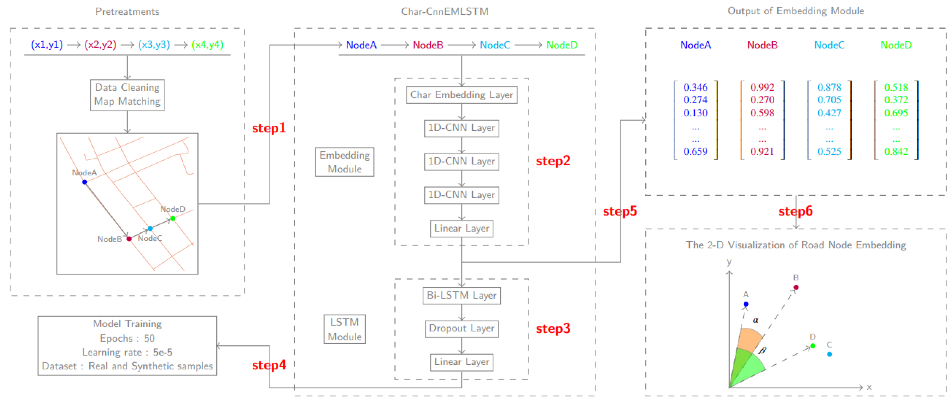
To sum up, the research flow of this paper is shown in Figure 1. This paper first assimilates nodes and travel route to words and sentence generated in the road network, respectively (shown as step 1 in Figure 1). Secondly, a deep learning embedding model StreetNode2VEC (shown as step 2 and step 3 in Figure 1) is proposed to map nodes into a low-dimensional space, thus generating a vector for each node. Thirdly, hyper-parameters of the StreetNode2VEC model are systematically calibrated on the basis of an experimental dataset and the objective of supervised learning (shown as step 4 in Figure 1). A total of five significant hyper-parameters are calibrated. Finally, the vectorized representation of nodes (shown as step 5 in Figure 1) is subject to three experiments (shown as step 6 in Figure 1) of visualization, similarity analysis, and link prediction. The validity of the StreetNode2VEC model is judged based on the results and discussions of these experiments.

2. Related Work

2.1. Traffic Incidents on Urban Road Networks

The formation and development of urban road networks are influenced by multiple factors, such as politics, economy, geography, climate, and population flow. For example, geography and climate determine the layout and topology of urban road networks, and flows of population produce traffic incidents when loaded into the network. In a study on traffic incidents and urban road networks, Mohan [14] analyzed the influence of intersection density and road types on road traffic fatality rates. They suggested that a city with wider roads and larger city blocks tends to have higher traffic fatality rates, while those with narrower roads and smaller blocks have lower traffic fatality rates. Xie [15] confirmed the spatial dependence of road traffic accidents between adjacent intersections using data of 195 signalized intersections along 22 corridors in the urban areas. Zeng [16] considered not only the spatial correlation between intersections, but also the spatial correlation between adjacent sections and intersections to simulate the occurrence of road traffic accidents. Francesca [17] considered road and environmental conditions, and proposed a methodology for the calculation of urban branch road safety. Lee [18,19] integrated a comprehensive framework of pedestrian walking and fatalities and conducted the hotspot identification.. Giuseppe [20,21] focused on the risk analysis of collision between cyclist fatalities and vehicles in urban intersections. Traffic analysis zones (TAZs) are also used in road traffic accidents as an analysis method. Lee [22,23,24] explored a zone system for traffic safety and analyzed the at-fault driver features by the full use of macroscopic and microscopic safety data. And meanwhile the security hot-zones are identified. Xie [25] applied the traffic safety theory into the land use planning and evaluated the relationship between the traffic accidents and land use conversion. Soltani [26] identified the potential spatio-temporal distribution pattern of road traffic accidents by TAZs. Abdelaty [27] investigated the total crashes, severe crashes, and pedestrian crashes models for TAZs, block groups, and census tracts. Similar to the data type used in this paper, Stipancic [28] also used GPS data and surrogate safety measures, combined the two models to predict the severity level of road traffic accidents, and ranked them according to the predicted crash cost. Similar to the method used in this paper, deep learning is also used in traffic safety planning. Cai [29] used a high-resolution data acquisition framework and a deep learning structure of convolutional neural network to predict traffic accidents, and obtained higher accuracy. Marshall [30] considered features of street network in the analysis of road traffic accidents, including street network density, street connectivity along with street network pattern, and identified the impact of different road network features on road traffic safety.

2.2. Network Representation Learning

In real life, there are large quantities of unstructured data, such as texts, images, and videos. With regard to the collection, storage, and processing of unstructured data, progress have been made in various fields and industries. Text feature extraction means to extract the most representative information of a text as its features, and use simplified features in accomplishing relevant machine learning tasks. However, in face of massive text data, treating each text element as a feature would result in extremely high feature dimensions. In that case, the performance of algorithms designed using features with such dimensions would also be unacceptable.

n-Grams is a classic statistical text feature extraction method, which assumes that the n-th word in a sentence is correlated only with the $n-1$ words prior to it. Considering that n-Grams have too many parameters and require highly complicated computations, Bengio [31] proposed a method of distributed representation of words. This method uses artificial neural networks for model training, and increases model training speed through parameter sharing. Collobert [32] introduced a C&W model to generate word vectors. This model directly scores n-Gram phrases through constructing random phrases, instead of calculating conditional probability. For a phrase in the corpus, a high score is given by this model; for random phrases, a low score is given. In this way, the efficiency of model training is greatly increased. Inspired by Mikolov, [33] put forward a Skip-gram model, which also uses the current word of the training text to predict the context of the word and maps the unstructured current word as a vector. When two words having similar meanings are vectorized by the Skip-gram model, they have close distances in the embedding space and vice versa.

In recent years, deep learning has been widely used in graphic feature extraction, which has evolved from the methods of natural language processing. Perozzi [13] introduced a DeepWalk method, took graphic nodes as words following the idea of word embedding, and adopted RandomWalk to access graphic nodes, thus generating a node sequence. On this basis, he treated node sequences as sentences, and used the Skip-gram model and other neural network models to finish vectorized representation tasks. DeepWalk uses RandomWalk to generate samples, and is highly extendable, as it has introduced a customized deep learning model to complete graph embedding tasks. LINE [34], Node2vec [35], and Walklets [36] are all improved on the basis of DeepWalk. Nguyen [37] integrated the time dimension into the graph embedding method, and extracted features of dynamic graphs. Zhang [38] performed text classification using convolutional neural networks after character encoding of texts, and achieved a pretty high accuracy. Sun [39] came up with a CENE framework, likened content information to nodes, abstracted texts as graphs, and accomplished graph embedding tasks on this basis.

3. Feature Learning Framework

This paper proposes a model named StreetNode2VEC for the representation of nodes based on traffic data. The aim of StreetNode2VEC is to compile a dictionary, in which each vector corresponds to a node in the road network. The model can reflect node features in the road network, and help to better accomplish traffic tasks. Given that StreetNode2VEC can be used to carry out subsequent prediction and classification tasks, it is fair to say that the model is a byproduct of the completion of road-related prediction tasks. For this reason, to conduct node embedding, it is necessary to construct a reasonable synthetic task. When neural network training is completed, the parameters obtained are the vectorized representation results of nodes. The StreetNode2VEC model is comprised of an embedding module and a Bi-directional Long Short-term Memory Neural Network (Bi-LSTM) module. Specifically, the road network is obtained via Openstreetmap (an open source map website). Considering the encoding need for node numbers, the embedding approach of the character-level model is integrated into the StreetNode2VEC model, and naturally, the StreetNode2VEC model is analyzed in comparison with other embedding methods in the subsequent section. In the meanwhile, a Bi-LSTM module is incorporated into the StreetNode2VEC model for the reason of the advantages of a Long Short-term Memory Neural Network (LSTM) for handling sequence-based data.

3.1. Model Architecture

3.1.1. Character-Level Convolutional Neural Network

In this section, we will describe an embedding module (shown in Step 2, Figure 1) named character-level convolutional neural network (Char-Cnn). Convolutional neural network (CNN) is a high accuracy deep learning model for feature extraction and classification. Here, we define the road network in general as an undirected graph structure $G=(V,E)$, where node $v\in V$ represents the origin or destination of the road section and edge $e\in E$ represents the road section from node u to node v. Residents’ travel demands are met through the urban road network G, thus generating a travel route, e.g., a set of node sequences $tr=[u_1,u_2,\dots ,u_n]$. This is consistent with the process and principle of RandomWalk. Given a travel route $tr=[u_1,u_2,\dots ,u_n]$ as input raw sample, $tr$ is mapped into real-valued vectors by the first layer of our architecture which will be described in this section. Each node $v\in V$ has a unique index $u_{key}\in K$, K is the set of indices, $\left|K\right|$ is the length of K. We define the index of node u as a sequence of numbers $[p_1,p_2,\dots ,p_l]$, where l is the length of node u, and $p_i\in 0,1,2,\dots ,9$. We consider that each $p_i$ is embedded into a d-dimensional vector space using a lookup table $F_C(·)$ as Equation (1):

$$\begin{array}{c}\hfill F_C\left(u_{key}\right)=C^{u_{key}}\end{array}$$

(1)

Here, $C\in {\mathbb{R}}^{d\times \left|K\right|}$ is a matrix of size $\left|K\right|\times d$ parameters. $C^{u_{key}}\in {\mathbb{R}}^{d\times l}$ is the $[p_1,p_2,\dots ,p_l]$-th columns of C and d is the dimension of index embedding. It is important to note that parameters of C are automatically updated during the learning process. So far, we have discussed the Index-level (or Char-level) representation of node u, and next we will deal with a one-dimensional convolutional neural network (1D-CNN).

A 1D-CNN performs a pipeline of extracting features on $C^{us{e}_{key}}$, the Index-level representation of node u, by using a filter $U\in {\mathbb{R}}^{d\times w}$ of width w. After we add a bias b and apply a nonlinear function to build a feature map $f^{u_{key}}\in {\mathbb{R}}^{l-w+1}$, $f^{u_{key}}$ is given by Equation (2):

$$\begin{array}{c}\hfill f^{u_{key}}=relu(U\otimes C^{u_{key}}[\ast ,i:i+w-1]+b)\end{array}$$

(2)

where $C^{u_{key}}[\ast ,i:i+w-1]$ is the i-to-$(i+w-1)$-th columns of $C^{u_{key}}$ and $A\otimes B=A^{T}B$. Suppose a 1D convolution layer has several filters $U_1,U_2,\dots ,U_m$, then $f^{u_{key}}=[f_1^{u_{key}},f_2^{u_{key}},\dots ,f_m^{u_{key}}]$ is the representation of the node u.

The 1D convolution layer can extract latent features with these filters instead of using manually feature selection. Subsequently, the 1D convolution layer usually is stacked so that lower layers can extract local features and more global features in subsequent ones.

3.1.2. Long Short-Term Memory Neural Network

An LSTM is a typical recurrent neural network, that is particularly suitable for dealing with sequential data. At time step t, given an input vector $x_t$ and a state vector $h_{t-1}$, the hidden state $h_t$ is obtained by a memory cell $C_t$, an input gate $i_t$, an output gate $o_t$, and a forget gate $f_t$. When data through several gate functions, the LSTM learns what information should be integrated or forgotten during the training process. An LSTM does the following as Equation (3):

$$\begin{array}{c}\hfill \begin{array}{cc}\hfill i_t& =\sigma (W_{xi}{x}_t+W_{hi}{h}_{t-1}+b_i)\hfill \\ \hfill f_t& =\sigma (W_{xf}{x}_t+W_{hf}{h}_{t-1}+b_f)\hfill \\ \hfill o_t& =\sigma (W_{xo}{x}_t+W_{ho}{h}_{t-1}+b_o)\hfill \\ \hfill C_t& =f_t\circ C_{t-1}+i_t\circ tanh(W_{xc}{x}_t+W_{hc}{h}_{t-1}+b_c)\hfill \\ \hfill h_t& =o_t\circ tanh\left(C_t\right)\hfill \end{array}\end{array}$$

(3)

where parameters of the LSTM are $W_{xj}$, $W_{hj}$, and $b_j$ for $j\in \{i,f,c,o\}$. $\sigma (·)$ and $tanh(·)$ are the element-wise Relu and tanh activation functions. ∘ is the element-wise multiplication operator. A Bi-directional LSTM (Bi-LSTM), an extension of traditional LSTM, is applied into our model architecture for improving model performance. Bi-LSTM extracts features more effectively than unidirectional LSTM [40]. Bi-LSTM contains forward unit $LST{M}_{forward}$ and backward unit $LST{M}_{backward}$, the parameters of the two units are independent of each other. Bi-LSTM will degenerate into an LSTM architecture without a backward unit. If the forward unit is cut off from the Bi-LSTM, it is simplified to a regular LSTM with reversed time axis results. Bi-LSTM extracts features from two directions in the training process, and finally merges the features from two directions. The hidden state $h_t^f$ at time t is obtained by running $h_{t-1}^f$ and $x_t$ through $LST{M}_{forward}$, and the hidden state $h_t^b$ is obtained by running $h_{t+1}^b$ and $x_t$ through $LST{M}_{backward}$. Finally, two tensors $h_t^f$ and $h_t^b$ are concatenated for prediction. The final output $h_t$ of Bi-LSTM at time t is $[h_t^f,h_t^b]$. The architecture of this section, or Bi-LSTM module, is summarized in Step 3, Figure 1.

3.1.3. StreetNode2VEC Model

This paper designs a StreetNode2VEC model, which integrates an embedding module and a Bi-LSTM module. The integration of two modules requires a specific design, as each module has unique architecture and advantages. By inputting a node into the Char-Cnn embedding module and extracting its features using the Bi-LSTM module, we can ultimately employ a fully connected layer to output the classification of this node.

• Pretreatments: Data cleaning, map matching, and other pretreatments are executed in this step. The longitude and latitude sequences of GPS are converted into a route composed of road nodes, and the nodes are put through one-hot encoding as inputs of the next step.
• Embedding module: The Char-Cnn embedding model is used in this step to prepare the data required by the Bi-LSTM layer. After being vectorized, the nodes on the route are transferred to the next step as inputs.
• Bi-LSTM module: The Bi-LSTM layer and the Maxpool layer are used in this step to extract the advanced features of data, the fully connected layer is adopted to adjust the output size of data, and eventually the binary classification results of the route are output.

3.2. Detailed Model Settings

3.2.1. Construction of Synthetic Samples

Synthetic samples absent from the dataset are generated according to the discussions in related studies [32,41,42], and both the synthetic samples generated and the real samples in the dataset are used to train the neural network model. The target of the model can be deemed as a binary classification task, that is, to determine whether an input sample received is a real or synthetic sample. Following this idea, we construct a synthetic task to complete training and extract node features.

To keep a dataset balanced, we generate a dataset in which real and synthetic samples are equal in quantity. For each route, m nodes are randomly selected from the route, and each of these nodes is replaced by a random node in the road network. Here, m is $30\%$ of the length of the route.

3.2.2. Parameters of the Embedding Module

This paper deals with a classification problem, and the detailed parameter calibration process is described in Section 3.3. We use a Char-Cnn layer to convert nodes into vectors with a dimension of 128. The conversion dimension of each character d is 128. There are three 1D-CNN layers. The numbers of filters m are 120 and filter size is uniformly 5. After feature extraction using 1D-CNN, a Maxpool layer is used to reduce data dimensions. Each 1D-CNN layer adopts the rectified linear function (ReLU). This function helps neural networks filter out unnecessary information in data flows to reduce network nonlinearity by setting negative inputs as 0. Regularization is performed to avoid overfitting of the deep learning model, and improve its generalization ability. In this paper, the dropout layer is adopted.

3.2.3. Parameters of the Bi-LSTM Module

The design of the Bi-LSTM module is relatively simple. A Bi-directional LSTM module is adopted in this paper, and the number of nodes in the hidden layer is 200. To avoid overfitting, we have also introduced the dropout layer into the Bi-LSTM module.

3.2.4. Parameters of Training Methods

When model parameters are optimized by an optimization algorithm, a loss function needs to be proposed to evaluate the performance of the model. As a result that the parameter calibration of the StreetNode2VEC model is considered as a classification task, cross entropy loss is adopted in this paper, as detailed in the following Equation (4).

$$\begin{array}{c}\hfill L=-[ylog\widehat{y}+(1-y)log(1-\widehat{y})]\end{array}$$

(4)

where L is the loss function, y is the label of the actual sample, and $\widehat{y}$ is the probability of the predictive sample. With the set loss function, the optimization algorithm of the model can be discussed. The neural network optimization algorithm is an algorithm developed to train neural networks. By training the weights and biases of the parameters of the iteration update model, it raises model accuracy. At present, a range of optimization methods are available for calculating model parameters. In this paper, the RMSProp algorithm is employed to calculate the differential squared weighted average of gradient. This approach can revise gradient direction, and reduce excessive fluctuations in training.

3.3. Model Training

The task of this section is to train the StreetNode2VEC model to achieve the best performance. For a machine learning model, the training of the model is based on the training dataset, the observation of the training accuracy is based on the validation dataset, and the performance evaluation of the model is finally based on the test dataset. The data source, data cleaning, and the construction of training, validation, and test sets of the dataset will be specified in Section 4.1. The accuracy of the model and the value of the loss function are used to evaluate the performance of StreetNode2VEC. Specifically, the value of the loss function is calculated by using cross entropy, while the accuracy is defined as the percentage of sample where all labels are correctly classified.

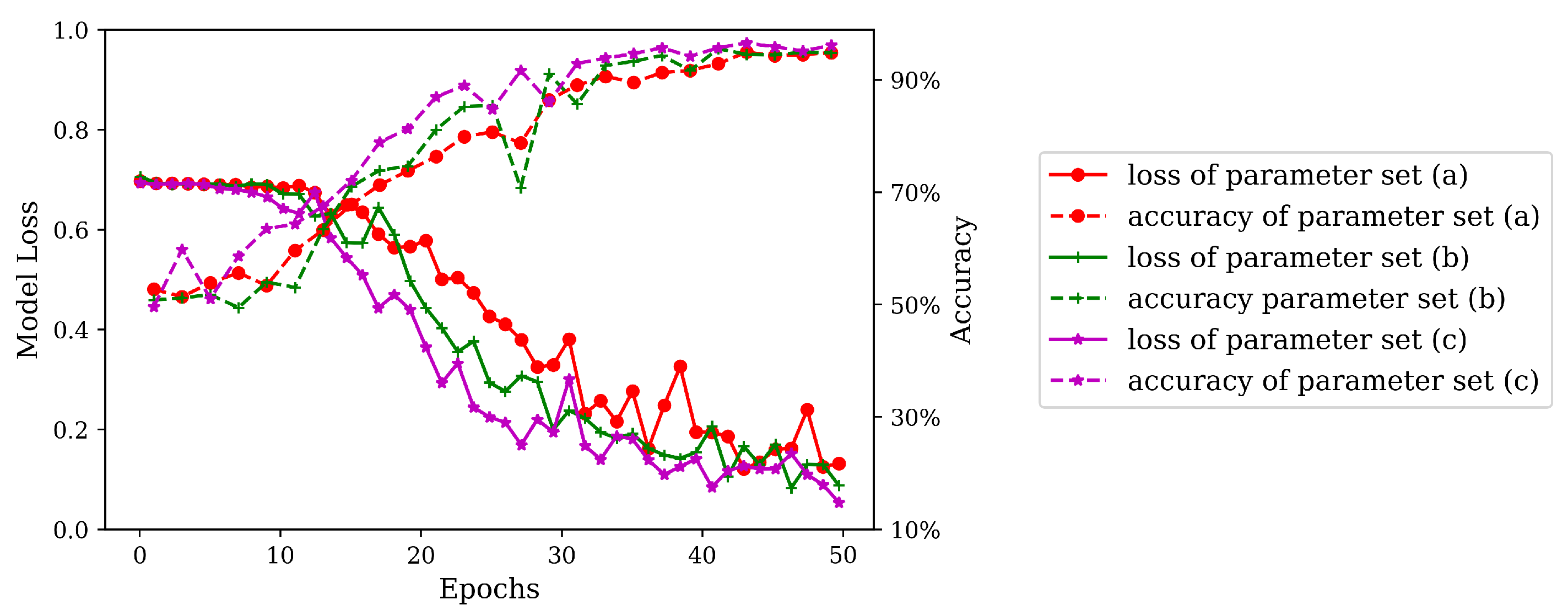
3.3.1. Model Parameter Calibration

In the word embedding model released on Glove’s official website [43], words are mapped to 25, 50, 100, 200, and 300-dimensional vector spaces. Referring to this model, this paper maps the nodes to 32, 64, and 128-dimensional vector spaces. In this section, we aim to test the performance of three parameter sets in training, i.e., embedding module output dimension, character dimension, and filter size. To that end, we will test three parameter sets: (a) embedding module output dimension is 32, character dimension is 32, filter sizes are (30, 30, 30); (b) embedding module output dimension is 64, character dimension is 64, filter sizes are (60, 60, 60); (c) embedding module output dimension is 128, character dimension is 128, filter sizes are (120, 120, 120). All of the three parameter sets are tested under a batch size of 32 and a learning rate of $5\times {10}^{-4}$. See the detailed training process in Figure 2.

As illustrated in Figure 2, in the training of the three sets of parameters, with the increase of epochs, the loss value of the training set gradually decreases with fluctuations, and the accuracy of the testing set continuously increases. After about 35 epochs, the three sets of parameters have an accuracy of above $90\%$. Among them, parameter set (a) has the poorest performance, lowest accuracy, and most intense fluctuations in loss value in training, whereas parameter set (c) has the optimal performance. It can thus be known that, the higher the character embedding dimension, the better the model training performance. The conclusion of this experiment is consistent with the conclusion drawn in [41]. For this reason, parameter calibration is performed on the basis of parameter set (c) in subsequent experiments.

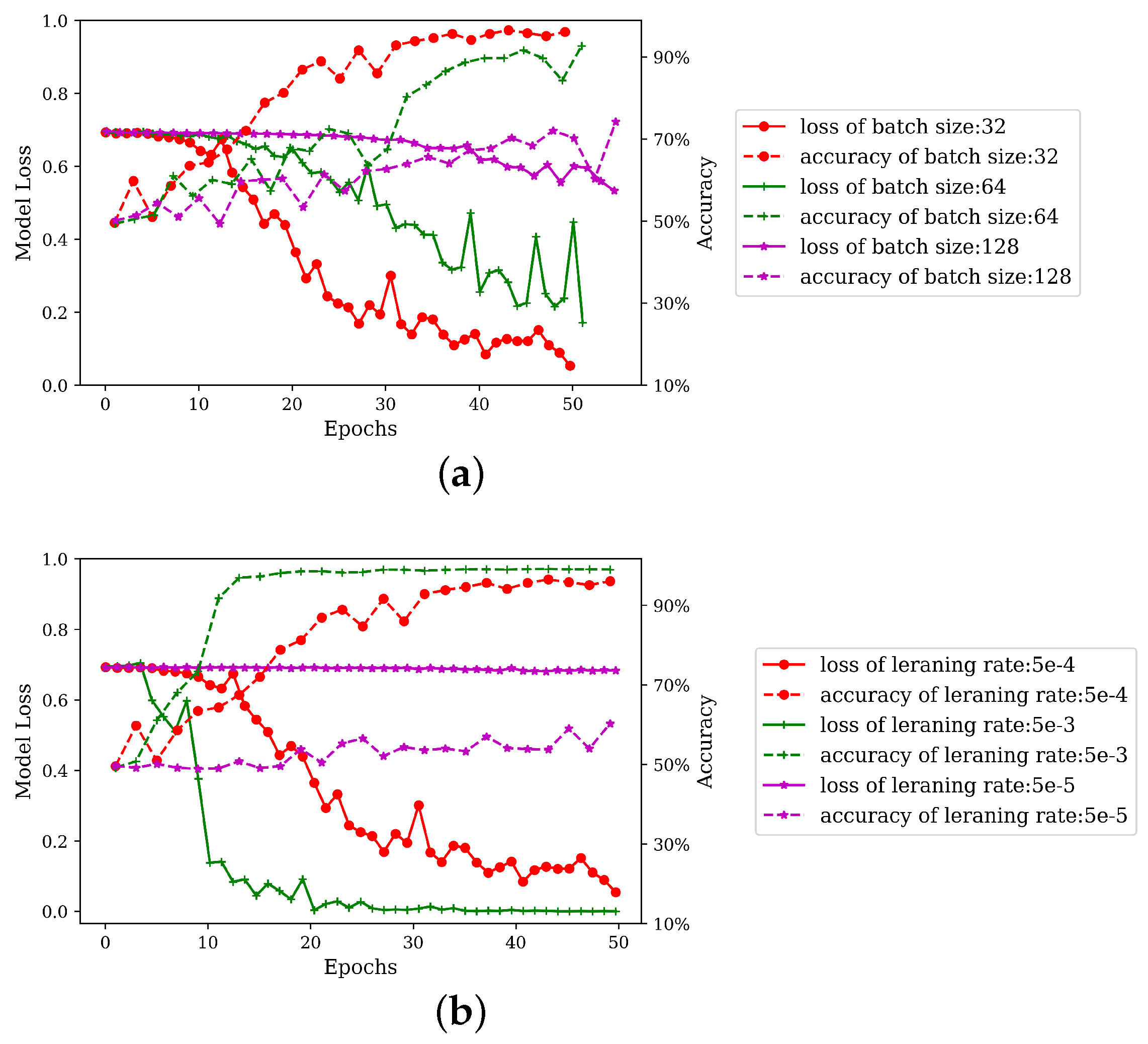
3.3.2. Training Parameter Calibration

The updating of model parameter requires multiple epochs, and, in each iteration, model parameters are updated using a back propagation algorithm. In normal circumstances, too few epochs result in inadequate training, while too many epochs lead to overfitting. In machine learning, the general condition for epoch termination is when the loss function value of the validation set reaches the minimum [44]. As shown in Figure 2, after 40 epochs, the accuracy of the testing set tends to be stable, so the number of epochs is uniformly set as 50 in this experiment.

In model training, both learning rate and batch size have very significant effects on model performance. To be specific, an excessively high learning rate causes continuous fluctuations in the loss function value, whereas an excessively small learning rate gives rise to excessively slow convergence. A large batch size is capable of avoiding intense fluctuations in loss and increasing model training speed, but may be easily trapped in “local minimum”. Generally speaking, this problem can be avoided by gradually increasing batch size within the range allowed by machine performance. Details about the parameter calibration of learning rate and batch size are given in Figure 3.

As can be known from Figure 3a, learning rate is set as $5\times {10}^{-4}$, and when batch size reaches 128, the course of model training is almost stagnant. Thus, within the range allowed by machine performance, batch size should not exceed 128, and should be continuously reduced. When batch size is 32, there is a satisfactory training effect. In Figure 3b, batch size is uniformly set as 32. When learning rate is lower than $5\times {10}^{-5}$, training speed becomes too low, so learning rate is increased. When learning rate reaches $5\times {10}^{-3}$, the model has a relatively high convergence speed. To sum up, parameter set (c) is selected as the parameters of the model. In training, batch size is set as 32, and learning rate as $5\times {10}^{-3}$.

4. Case Study

4.1. Dataset Process

The dataset of taxi trajectory in Porto [45] derived from ECML/PKDD 15: Taxi Trajectory Prediction, is used in this paper. It records the GPS trajectories of 442 taxis in Porto from July 2013 to June 2014. The dataset provides the taxi GPS trajectories in the process of carrying passengers, rather than in the process of seeking passengers. $T=\left\{\{longitud{e}_i,latitud{e}_i,\}\right|i=1,2,\dots ,n\}$ discretely reflects the location information of passengers and expresses their travel demand, which is necessary for traffic safety planning. Then the passengers’ travel routes can be obtained based on the Map Matching method, which will be input into the StreetNode2VEC model.

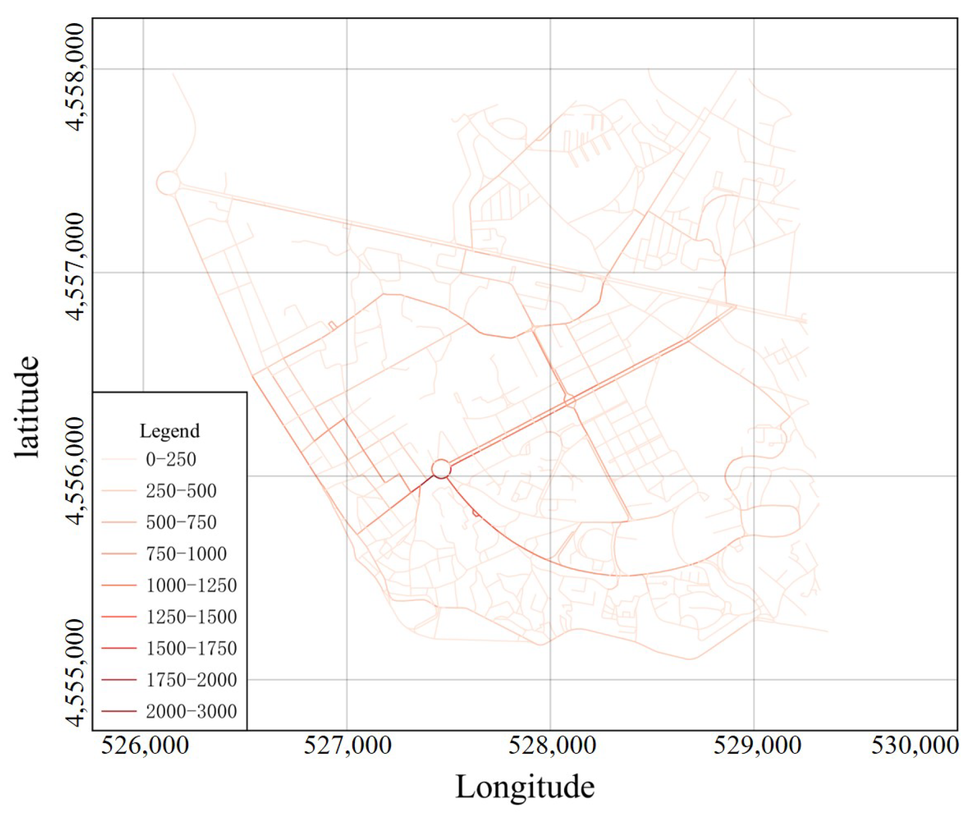
Limited by machine performance, in the training dataset of this dataset we select the boxes within the longitude and latitude scope of $[-8.69157,-8.64963,41.14628,41.17128]$, which cover an area of about 9.5 km${}^2$. Next, we use Openstreetmap to extract the road networks within this scope. The Python environment provided in Qgis3 is adopted for the batch processing of GPS data, and Qgis plugin employed to map GPS trajectory points to the network using the Hidden Markov model and the Viterbi algorithm. Finally, by counting the number of road sections in the routes and removing the shorter routes, we obtain a total of 8286 travel routes, which pass through a total of 262,903 road sections, as shown in Figure 4.

Figure 4 shows that road sections darker in color have a higher selection frequency. Primary roads have darker colors, while secondary roads have lighter ones. More than 1000 road sections have a selection frequency of less than 500, and only a few have a significantly higher selection frequency. This paper takes 8286 travel routes as real routes, and generates 8286 synthetic routes according to Section 4.1. The sample set has a total of 16,572 entries of data, which constitute the dataset D of this paper. On this basis, the dataset is scrambled into three subsets by a ratio of 6:2:2, i.e., training set $D_{train}$, validation set $D_{eve}$, and testing set $D_{test}$. The training set has 9943 entries of data, while the validation set and the testing set each have 3315 entries. Furthermore, the ratio of real to synthetic data is balanced in each subset.

4.2. Experimental Setup

For the visualization task, visualizing the output of the embedding model offers the most direct approach for understanding the effect of the embedding model. In this paper, we map the output results of StreetNode2VEC (as step 5 in Figure 1) to a two-dimensional space according to the TSNE [46] method, thus realizing visualization (as step 6 in Figure 1). In the two-dimensional space, nodes having similar semantics are close to each other. The visualization method can thus evaluate the embedding model results in an intuitive manner. We first map data as 128-dimensional vectors using the model, and then map them to a two-dimensional space for visualization by the TSNE method. For similarity analysis task, this paper maps road network nodes as 128-dimensional vectors. When it comes to computation between vectors, a common method is to calculate the cosine value between two vectors. Given a node u, the first task is to find a node v, whose direction is the same as, opposite to, or vertical with the direction of u, as expressed by Equations (5)–(7):

$$\begin{array}{c}\hfill v^{*}=\underset{v\in V\backslash v}{argmin}|cos(v,u)-1|\end{array}$$

(5)

$$\begin{array}{c}\hfill v^{*}=\underset{v\in V\backslash v}{argmin}|cos(v,u)+1|\end{array}$$

(6)

$$\begin{array}{c}\hfill v^{*}=\underset{v\in V\backslash v}{argmin}|cos(v,u)|\end{array}$$

(7)

Here u and v are 128-dimensional vectors of node u and v. When the cosine value $cos(u,v)\in [-1,1]$ between vectors u and v is 1, it means that the two vectors have the same direction; when it is −1, it means that they have opposite directions; when it is 0, it means that they are vertical with each other.

Link prediction in social networks is developed to predict whether two persons are linked, or will be linked in the future. Naturally, in road networks, link prediction is used to predict whether two nodes are linked, or will be linked in the future. In this section, a simple binary classification task is constructed. For the dataset in Section 4.1, there are 1233 pairs of links in set E. Similarly, we randomly extract 1233 disconnected node pairs as synthetic samples. It has a total of 2466 samples (real and synthetic samples each accounting for 50%), and is divided into three subsets by the ratio of 6:2:2. The training set has 1478 entries of data, while the validation set and the testing set each have 494 entries. Furthermore, the ratio of real to synthetic data is balanced in each subset.

For each sample, we concatenate the two vectors of nodes as the edge feature and then build a support vector machine binary classifier to fulfill the classification task. Moreover, for the two vectors of nodes, we calculate their element-wise product in

Table 1. Element-wise operators.

Element-Wise Product	Formula of Element-Wise Product
Average	$(u+v)/2$
Hadamard	$u\ast v$
L1	$|u+v|$
L2	${(u-v)}^2$

.

ROC curve and AUC score are used to evaluate the performance of classifiers, so as to evaluate different embedding methods, such as Node2vec and graph convolutional network (GCN) [47]. According to Section 3.2, the StreetNode2VEC maps road network nodes as 128-dimensional vectors. For Node2vec and GCN, the dimension of the embedding is set as 128. Furthermore, we tune 1 to 2 significant hyper-parameters for the embedding methods via Gridsearch.

4.3. Results of Visualization

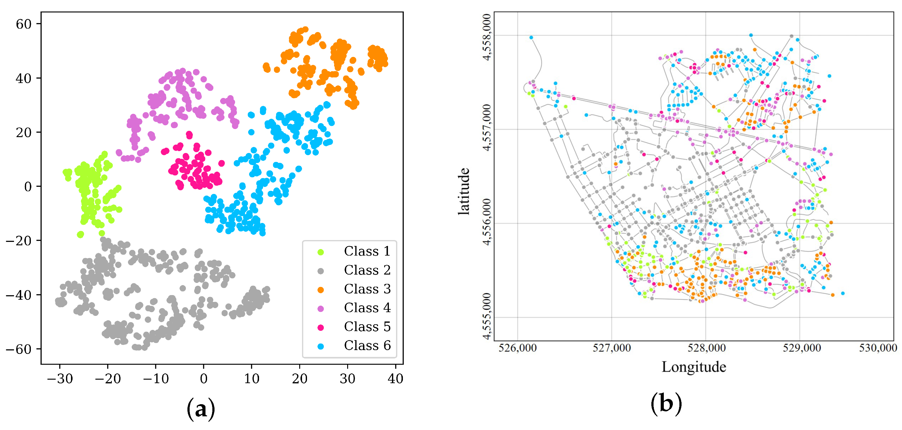
According to Figure 5, road network nodes present a clustered distribution pattern, suggesting that the model has distinctively differentiated nodes with different features. Here we artificially classify the nodes into six types, and assign different colors to them.

To be specific, Figure 5a,b have consistent node colors. Figure 5b shows the visualization of the six types of nodes on the map. It can be seen that different colors are underlined in different manners in different regions. The nodes in Orchid correspond in large quantities to the Porto’s main road Avenida da Boavista and neighbor nodes. Those in green, yellow, and dark orange are concentrated in the south of this region, and some of the nodes in dark orange are located in the northeast. Dark gray nodes correspond in large quantities to the roads in the middle. There are no obvious distribution features of deep sky blue nodes in Figure 5b, and they are mainly concentrated in the north and south, and scattered in Figure 5a as well. In the four-step travel demand prediction, TAZs are the basic spatial unit. The division of TAZs is based on the spatial clustering of one or more census blocks. The vectorized nodes contribute to the division of traffic zones in traffic planning [48], making it more compatible with residents’ travel habits. It can be seen from Figure 5b that travelers’ travel routes have imperceptibly divided the road network into different regions.

We can use the results to subdivide the TAZs with StreetNode2VEC, so as to form traffic safety analysis zones. More specifically, the traditional TAZ division often takes the arterial roads into account. Once the crashes occur on these boundary roads of the adjacent TAZs, the traffic safety modeling only based on the characteristics of a zone could be invalidated. Differently, the StreetNode2VEC method considering the residents’ travel routes can extract the characteristics of each node and these nodes will show spatial clustered pattern according to the results of visualization. By introducing the node clustering results, the TAZ boundaries can be softened. Then the traffic safety analysis zones (TSAZs) will be obtained, which are the more reasonable units for analyzing the traffic incidents and implementing the traffic safety planning.

4.4. Results of Road Nodes Similarity Analysis

As shown in

Table 2. Similarity analysis of road nodes.

$cos(A,B)=0.919$ $cos(A,C)=-0.460$ $cos(A,D)=0.004$
$cos(A,B)=0.997$ $cos(A,C)=-0.933$ $cos(A,D)=0.001$

, we take two intersections as examples. One is the intersection between Praca de Liege Road and Rua do Faial Roa (point A in the first row of Table 2), and the other is the intersection between Rua da Fonte da Moura Road and Rua da Cidade de Mindelo Road (point A in the second row of Table 2).

Among all the points $v\in V\backslash A$, the cosine value between points B/C/D and point A is closest to 1/−1/0. As can be seen from Table 2, the cosine value between point B and point A is closest to 1. The two points happen to have similar positions and service regions in the road network and show mutual complementation and overlap. The cosine value between point C and point A is closest to −1, and there is no overlap between their service scopes. Points D and A have an included angle of ${90}^{\circ }$, and undertake different tasks in the road network (point A is mainly responsible for gathering and distribution, and point D is for connecting). This section demonstrates that the vectorized nodes have extracted the spatial features and nodal functions of the road network. They can also assume nodal functional partitioning, similarity matching, and other traffic tasks. In the existing traffic safety planning, the occurrence probability of traffic accidents is calculated though the analysis of the intersection types, accident types, speed limits, and pedestrian impacts. Remarkably, by combining the traffic accident data and the above node vectorization results, the traffic safety characteristics and residents’ travel habits will be considered simultaneously. Moreover, through the similarity calculation, the nodes with same or different features will be identified. The forecasting algorithm, such as machine learning, can also be used to detect the accident black spots.

4.5. Results of Road Nodes Link Prediction

For the StreetNode2VEC model, we select Node2vec as our baseline. As can be seen from

Table 3. Results of urban road network link prediction.

Model Name	AUC Score
	Average	Hadamard	L1	L2
Node2vec	0.503	0.749	0.711	0.656
GCN	0.609	0.825	0.752	0.711
StreetNode2VEC	0.772	0.785	0.818	0.803

, compared with Node2vec on different operators, StreetNode2VEC has achieved 4.8–51% improvement in terms of AUC score. For the GCN model, the AUC scores based on Average, L1, and L2 are worse than those of StreetNode2VEC, except for the AUC score based on Hadamard.

For different operators in Table 1, StreetNode2VEC gets a higher AUC score on Average, L1, and L2. For all embedding methods, only AUC scores on four different operators of StreetNode2VEC are all higher than 0.75. This suggests that, regardless of the specific operators used, when we provide a random node pair $(u,v)$ to the classifier, the StreetNode2VEC will reach a conclusion about whether a link should be established for the node pair. If the classifier concludes that a link should be established to connect two nodes, the conclusion will have a credibility probability of 75%; if not, the conclusion will have a credibility probability of 75%. This indicates that the embedding of StreetNode2VEC is more credible.

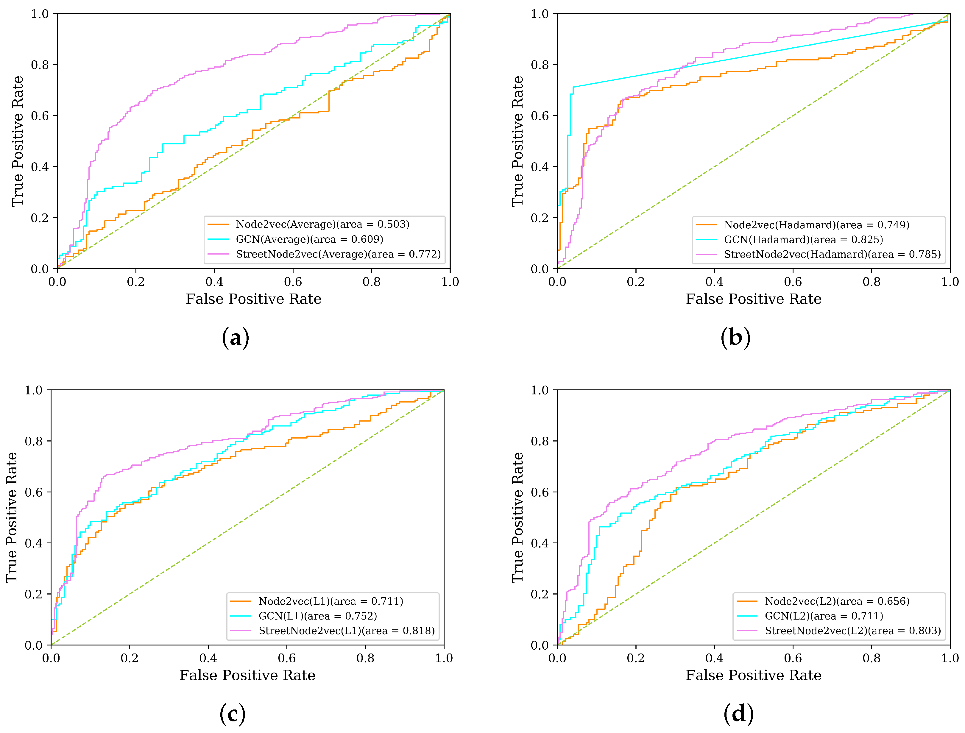
As shown in Figure 6, ROC curves of three diverse models on four different operators are used to evaluate the performance of the link prediction task. We can see from Figure 6a that the performance of StreetNode2VEC far exceeds that of the other two models when the operator is Average. For Figure 6b,c, it is clear that both Hadamard and L1 are satisfactory operators in the application of the three embedding models. As seen in Figure 6d, operator L2 performs poorly compared to L1 in the three embedding models. From the perspective of four different operators, Hadamard and L1 are relatively applicable to the three models tested in the vectorized representation task of road network nodes. From the perspective of the three models, StreetNode2VEC is relatively unaffected by operator types. Seen from traffic planning, if an engineer uses the traditional four-step travel demand model for traffic planning, the engineer will have to constantly test the trip assignment results of different schemes in the fourth step (trip assignment). In this case, the high-credibility link prediction technique provided in this section can help the engineer integrate residents’ travel habits into the future road planning. Link prediction can be widely used in traffic safety planning, such as the discovery of safe travel paths. For accident-prone nodes or sections, link prediction can provide quantitative reference as to whether a safe travel path should be established in the public transport or other transportation hubs. At the same time, for the transit route given by the public transport planning, the route safety index can be calculated by aggregation according to the node features.

5. Conclusions and Future Directions

Inspired by the idea of word embedding in Natural Language Processing, this paper proposes an urban road node embedding model combining urban road networks and residents’ travel data, together with the corresponding calculation flow. Through model parameter calibration, node vectors are obtained. On this basis, the tasks of visualization, similarity computation between road network nodes, and link prediction are carried out.

1. Residents engage in daily travels under the constraints of urban road networks and land use types, and their travel routes have imperceptibly divided the road network into different regions. In traffic analysis zones(TAZs), we are supposed to divide a region into different traffic zones. The conclusion of this paper suggests that the division of traffic zones is not only methodologically necessary, but also compatible with residents’ travel habits. Meanwhile, the nodes in vectorized representation can help engineers optimize the TSAZ division. Taken the node clustering results into account, the TSAZs associated with residents’ travel habits and network structure will be acquired on the basis of the existing TAZs. Then the features of different TSAZs can be integrated to conduct the hot zone identification.

2. This paper performs the similarity computation between road network nodes after embedding, so that the road network nodes can be compared with each other. According to the research results, the vectorized nodes still retain their road network features, and can be used to differentiate nodes associated with different functions in the road network. The nodal functional partitioning results obtained through traveler’s travel data can subdivide an urban road network, intersection, and a straight stretch of road. The node vectorization results are extended with the traffic accident data. By comparing the similarity between the accident black spots and other intersections, the intersections with potential safety hazard will be figured out. This method can be used to forecast the potential black spots.

3. On the basis of the representation of road network nodes in vector spaces, this paper performs link prediction, and achieves satisfactory scores. Clearly, when the economy, population, and residents’ travel habits of a city remain basically constant, link prediction can be used to predict whether a link should be established between two nodes. This result can reflect travelers’ intentions about the establishment of a node to node link. The method can not only help engineers conduct the medium and short-term planning of road networks, but also be used to launch large-capacity traffic modes in segments and intersections with strong demands. Additionally, focusing on the traffic safety planning, the node vectorization results merged with the traffic accident data can be input to the link prediction model to explore the potential safe travel paths. In the road traffic, the node characteristics can be used to evaluate and optimize the safety of the actual transit routes.

To summarize, this paper proposes the StreetNode2VEC method and analyzes the effectiveness and feasibility in Network Representation Learning. The vectorized nodes integrating the traffic safety data are helpful for traffic safety planning, including the TSAZ division, accident black spot identification, evaluation and optimization of safe travel routes, and so on. However, limited by the lack of traffic safety data in the current research area, other regions with more complete multi-source data can be found for further study. The study and discussion of node vectorized representation under different time periods in this paper are missing, mainly because the time span of our dataset is up to one year. In response, we will analyze node vectorized representation under different time periods in future research. Additionally, StreetNode2VEC can represent dynamic demand matrices used in traffic planning and management. In addition, under the limitation of the data size, the flow of some road segments (obtained by aggregating travel routes) is low, so comparative analysis in this paper does not extend to the relevant methods of traffic prediction. We can analyze other travel datasets to improve and reinforce experimental results in the future.

References

- World Health Organization. Global status report on road safety 2018: Summary. Available online: https://apps.who.int/iris/handle/10665/277370 (accessed on 15 November 2020).
- Sayed, T.; Rodriguez, F. Accident Prediction Models for Urban Unsignalized Intersections in British Columbia. Transp. Res. Rec. J. Transp. Res. Board 1999, 1665, 93–99. [Google Scholar] [CrossRef]
- Greibe, P.; Rodriguez, F. Accident prediction models for urban roads. Accid. Anal. Prev. 2003, 35, 273–285. [Google Scholar] [CrossRef]
- Mountain, L.; Fawaz, B.; Jarrett, D. Accident prediction models for roads with minor junctions. Accid. Anal. Prev. 1996, 28, 695–707. [Google Scholar] [CrossRef]
- Lee, J.; Abdel-Aty, M.; Jiang, X. Multivariate crash modeling for motor vehicle and non-motorized modes at the macroscopic level. Accid. Anal. Prev. 2015, 78, 146–154. [Google Scholar] [CrossRef]
- Lee, J.; Abdel-Aty, M.; Cai, Q.; Wang, L.; Huang, H. Integrated modeling approach for non-motorized mode trips and fatal crashes in the framework of transportation safety planning. Transp. Res. Rec. 2018, 2672, 49–60. [Google Scholar] [CrossRef]
- Mussone, L.; Ferrari, A.; Oneta, M. An analysis of urban collisions using an artificial intelligence model. Accid. Anal. Prev. 1999, 31, 705–718. [Google Scholar] [CrossRef]
- Singh, G.; Pal, M.; Yadav, Y.; Singla, T. Deep neural network-based predictive modeling of road accidents. Neural Comput. Appl. 2020, 32, 1–10. [Google Scholar] [CrossRef]
- Anderson, T.K. Kernel density estimation and K-means clustering to profile road accident hotspots. Accid. Anal. Prev. 2009, 41, 359–364. [Google Scholar] [CrossRef]
- Theofilatos, A. Incorporating real-time traffic and weather data to explore road accident likelihood and severity in urban arterials. J. Saf. Res. 2017, 61, 9–21. [Google Scholar] [CrossRef]
- Cameron, M.H.; Elvik, R. Nilsson’s Power Model connecting speed and road trauma: Applicability by road type and alternative models for urban roads. Accid. Anal. Prev. 2010, 42, 1908–1915. [Google Scholar] [CrossRef]
- Congiu, T.; Sotgiu, G.; Castiglia, P.; Azara, A.; Piana, A.; Saderi, L.; Dettori, M. Built environment features and pedestrian accidents: An Italian retrospective study. Sustainability 2019, 11, 1064. [Google Scholar] [CrossRef]
- Perozzi, B.; Al-Rfou, R.; Skiena, S. Deepwalk: Online learning of social representations. In Proceedings of the 20th ACM SIGKDD International Conference on Knowledge Discovery and Data Mining, New York, NY, USA, 24–27 August 2014; pp. 701–710. [Google Scholar]
- Mohan, D.; Bangdiwala, S.I.; Villaveces, A. Urban street structure and traffic safety. J. Saf. Res. 2017, 62, 63–71. [Google Scholar] [CrossRef] [PubMed]
- Xie, K.; Wang, X.; Ozbay, K.; Yang, H. Crash frequency modeling for signalized intersections in a high-density urban road network. Anal. Methods Accid. Res. 2014, 2, 39–51. [Google Scholar] [CrossRef]
- Zeng, Q.; Huang, H. Bayesian spatial joint modeling of traffic crashes on an urban road network. Accid. Anal. Prev. 2014, 67, 105–112. [Google Scholar] [CrossRef] [PubMed]
- Demasi, F.; Loprencipe, G.; Moretti, L. Road safety analysis of urban roads: Case study of an Italian municipality. Safety 2018, 4, 58. [Google Scholar] [CrossRef]
- Lee, J.; Abdel-Aty, M.; Huang, H.; Cai, Q. Transportation safety planning approach for pedestrians: An integrated framework of modeling walking duration and pedestrian fatalities. Transp. Res. Rec. 2019, 2673, 898–906. [Google Scholar] [CrossRef]
- Lee, J.; Abdel-Aty, M.; Choi, K.; Huang, H. Multi-level hot zone identification for pedestrian safety. Accid. Anal. Prev. 2015, 76, 64–73. [Google Scholar] [CrossRef]
- Cantisani, G.; Moretti, L.; De Andrade Barbosa, Y. Safety problems in urban cycling mobility: A quantitative risk analysis at urban intersections. Safety 2019, 5, 6. [Google Scholar] [CrossRef]
- Cantisani, G.; Moretti, L.; De Andrade Barbosa, Y. Risk analysis and safer layout design solutions for bicycles in four-leg urban intersections. Safety 2019, 5, 24. [Google Scholar] [CrossRef]
- Lee, J. Development of Traffic Safety Zones and Integrating Macroscopic and Microscopic Safety Data Analytics for Novel Hot Zone Identification. Ph.D. Thesis, University of Central Florid, Orlando, FL, USA, 2014. [Google Scholar]
- Lee, J.; Abdel-Aty, M.; Jiang, X. Development of zone system for macro-level traffic safety analysis. J. Transp. Geogr. 2014, 38, 13–21. [Google Scholar] [CrossRef]
- Lee, J.; Abdel-Aty, M.; Choi, K. Analysis of residence characteristics of at-fault drivers in traffic crashes. Saf. Sci. 2014, 68, 6–13. [Google Scholar] [CrossRef]
- Xie, B.; An, Z.; Zheng, Y.; Li, Z. Incorporating transportation safety into land use planning: Pre-assessment of land use conversion effects on severe crashes in urban China. Appl. Geogr. 2019, 103, 1–11. [Google Scholar] [CrossRef]
- Soltani, A.; Askari, S. Exploring spatial autocorrelation of traffic crashes based on severity. Inj. Int. J. Care Inj. 2017, 48, 637–647. [Google Scholar] [CrossRef] [PubMed]
- Abdel-Aty, M.; Lee, J.; Siddiqui, C.; Choi, K. Geographical unit based analysis in the context of transportation safety planning. Transp. Res. Part A Policy Pract. 2013, 49, 62–75. [Google Scholar] [CrossRef]
- Stipancic, J.; Miranda-Moreno, L.; Saunier, N.; Labbe, A. Network screening for large urban road networks: Using GPS data and surrogate measures to model crash frequency and severity. Accid. Anal. Prev. 2019, 125, 290–301. [Google Scholar] [CrossRef] [PubMed]
- Cai, Q.; Abdel-Aty, M.; Sun, Y.; Lee, J.; Yuan, J. Applying a deep learning approach for transportation safety planning by using high-resolution transportation and land use data. Transp. Res. Part A Policy Pract. 2019, 127, 71–85. [Google Scholar] [CrossRef]
- Marshall, W.E.; Garrick, N.W. Does street network design affect traffic safety? Accid. Anal. Prev. 2011, 43, 769–781. [Google Scholar] [CrossRef]
- Bengio, Y.; Ducharme, R.; Vincent, P.; Jauvin, C. A neural probabilistic language model. J. Mach. Learn. Res. 2003, 3, 1137–1155. [Google Scholar]
- Collobert Ronan, W.J. A unified architecture for natural language processing: Deep neural networks with multitask learning. In Proceedings of the 25th International Conference on Machine Learning, Helsinki, Finland, 5–9 July 2008; pp. 160–167. [Google Scholar] [CrossRef]
- Mikolov, T.; Sutskever, I.; Chen, K.; Corrado, G.S.; Dean, J. Distributed representations of words and phrases and their compositionality. In Advances in Neural Information Processing Systems; MIT Press: Cambridge, MA, USA, 2013; pp. 3111–3119. [Google Scholar]
- Jian, T.; Meng, Q.; Mingzhe, W.; Ming, Z.; Jun, Y.; Qiaozhu, M. LINE: Large-scale Information Network Embedding. In Proceedings of the 24th International Conference on World Wide Web, Florence, Italy, 18–22 May 2015; pp. 1067–1077. [Google Scholar] [CrossRef]
- Grover Aditya, L.J. node2vec: Scalable feature learning for networks. In Proceedings of the 22nd ACM SIGKDD International Conference on Knowledge Discovery and Data Mining, San Francisco, CA, USA, 24–27 August 2016; pp. 855–864. [Google Scholar] [CrossRef]
- Perozzi, B.; Kulkarni, V.; Skiena, S. Walklets: Multiscale graph embeddings for interpretable network classification. arXiv 2016, arXiv:1605.02115. [Google Scholar]
- Giang Hoang, N.; John Boaz, L.; Ryan, A.R.; Nesreen, K.A.; Eunyee, K.; Sungchul, K. Continuous-Time Dynamic Network Embeddings. In Proceedings of the Companion Proceedings of the Web Conference 2018, Lyon, France, 23–27 April 2018; pp. 969–976. [Google Scholar] [CrossRef]
- Zhang, X.; Zhao, J.; LeCun, Y. Character-level convolutional networks for text classification. In Advances in Neural Information Processing Systems; MIT Press: Cambridge, MA, USA, 2015; pp. 649–657. [Google Scholar]
- Sun, X.; Guo, J.; Ding, X.; Liu, T. A general framework for content-enhanced network representation learning. arXiv 2016, arXiv:1610.02906. [Google Scholar]
- Graves, A.; Schmidhuber, J. Framewise phoneme classification with bidirectional LSTM and other neural network architectures. Neural Netw. 2015, 18, 602–610. [Google Scholar] [CrossRef] [PubMed]
- Mikolov, T.; Chen, K.; Corrado, G.; Dean, J. Efficient estimation of word representations in vector space. arXiv 2013, arXiv:1301.3781. [Google Scholar]
- Goodfellow, I.; Pouget-Abadie, J.; Mirza, M.; Xu, B.; Warde-Farley, D.; Ozair, S.; Courville, A.; Bengio, Y. Generative adversarial nets. In Advances in Neural Information Processing Systems; MIT Press: Cambridge, MA, USA, 2014; pp. 2672–2680. [Google Scholar]
- Pennington, J.; Socher, R.; Manning, C.D. GloVe: Global Vectors for Word Representation. In Proceedings of the 2014 Conference on Empirical Methods in Natural Language Processing, Doha, Qatar, 26–28 October 2014; pp. 1532–1543. [Google Scholar]
- Lutz, P. Early stopping-but when? In Neural Networks: Tricks of the Trade; Springer: Berlin/Heidelberg, Germany, 1998; pp. 55–69. [Google Scholar]
- Kaggle. ECML/PKDD 15: Taxi Trajectory Prediction (I). Available online: https://www.kaggle.com/c/pkdd-15-predict-taxi-service-trajectory-i/ (accessed on 15 November 2020).
- Maaten, L.V.D.; Hinton, G. Visualizing data using t-SNE. J. Mach. Learn. Res. 2008, 9, 2579–2605. [Google Scholar]
- Kipf, T.; Welling, M. Semi-Supervised Classification with Graph Convolutional Networks. arXiv 2016, arXiv:1609.02907. [Google Scholar]
- O’Flaherty, C.A. Highways. In Traffic Planning and Engineering; Edward Arnold: London, UK, 1986; Volume 1. [Google Scholar]