Artificial Neural Network Optimized with a Genetic Algorithm for Seasonal Groundwater Table Depth Prediction in Uttar Pradesh, India


Abstract
1. Introduction
2. Materials and Methods
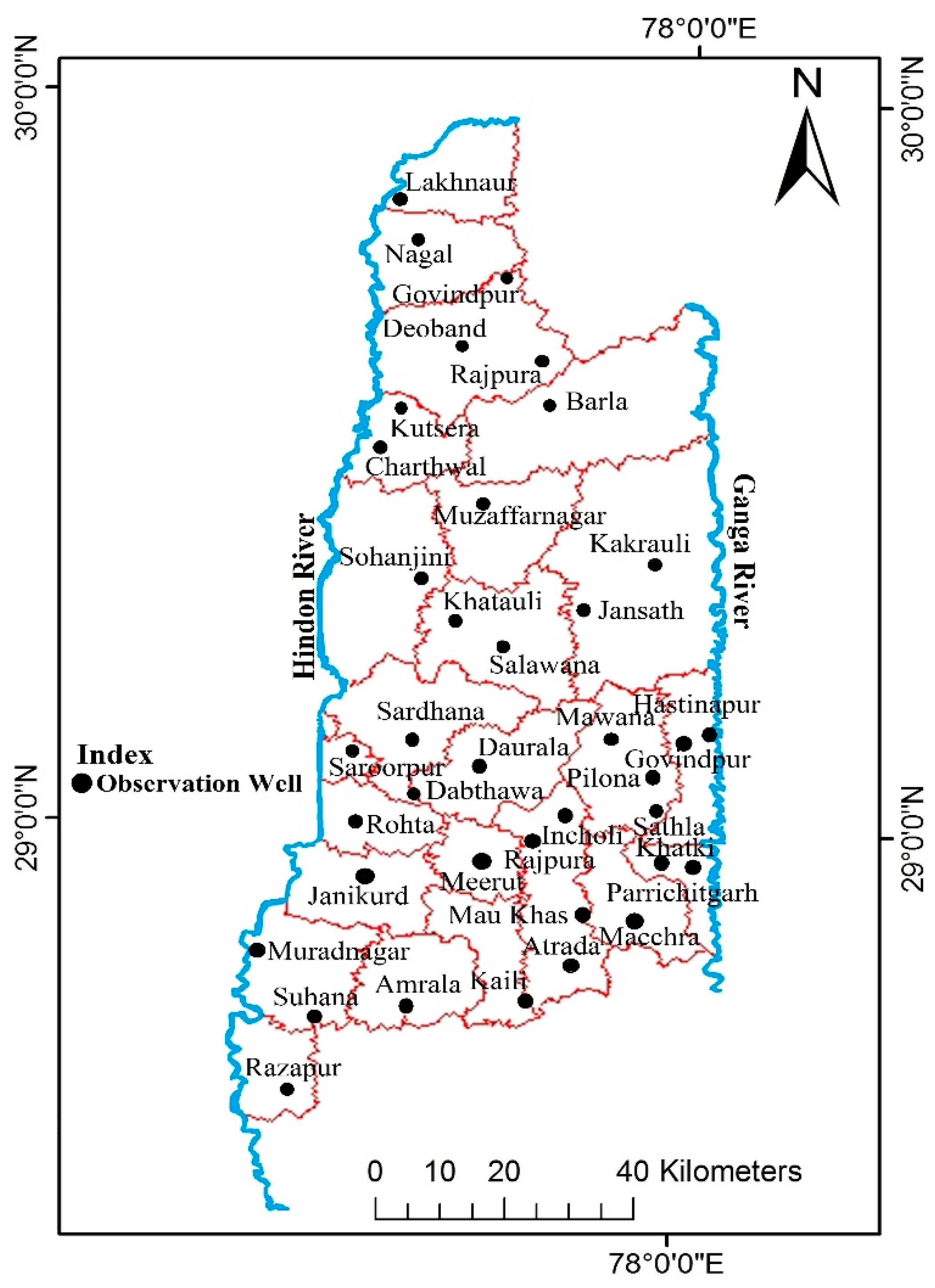
2.1. Description of the Study Area
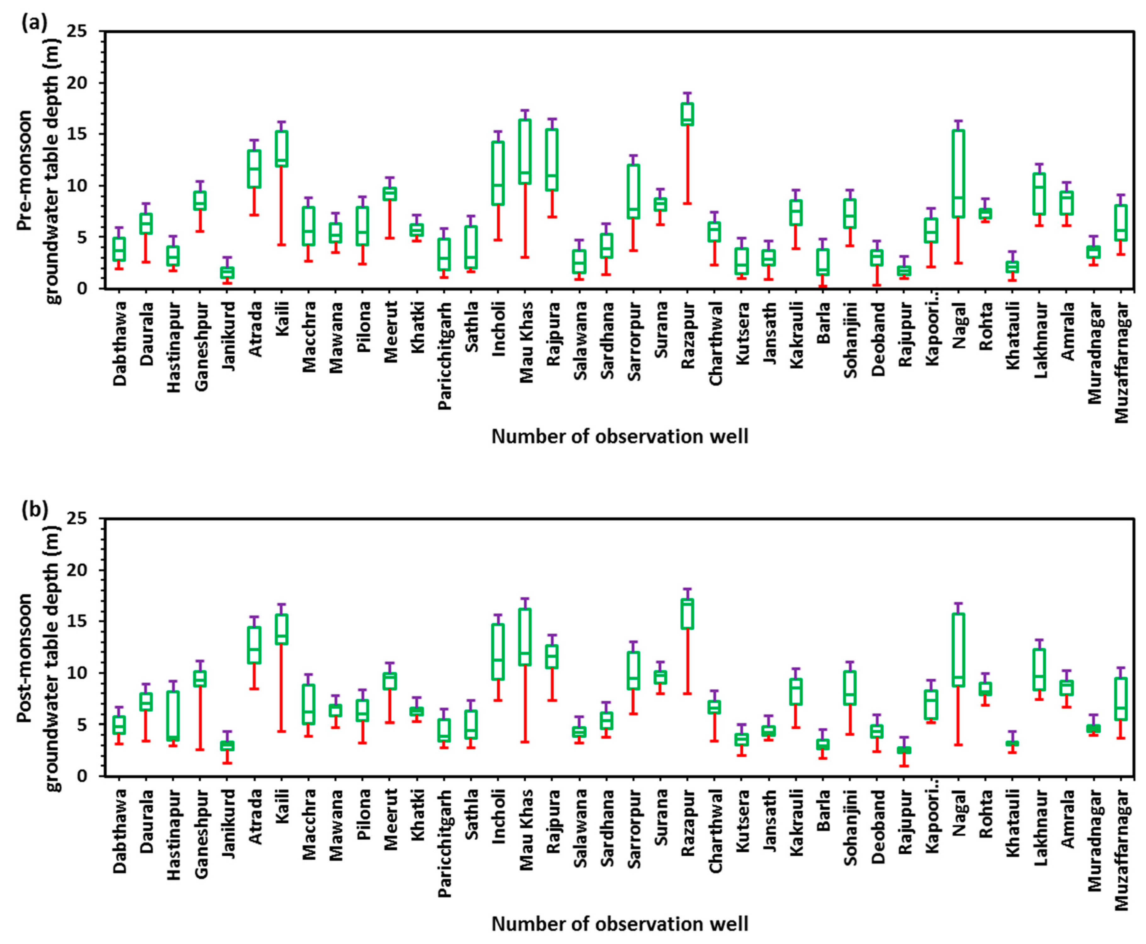
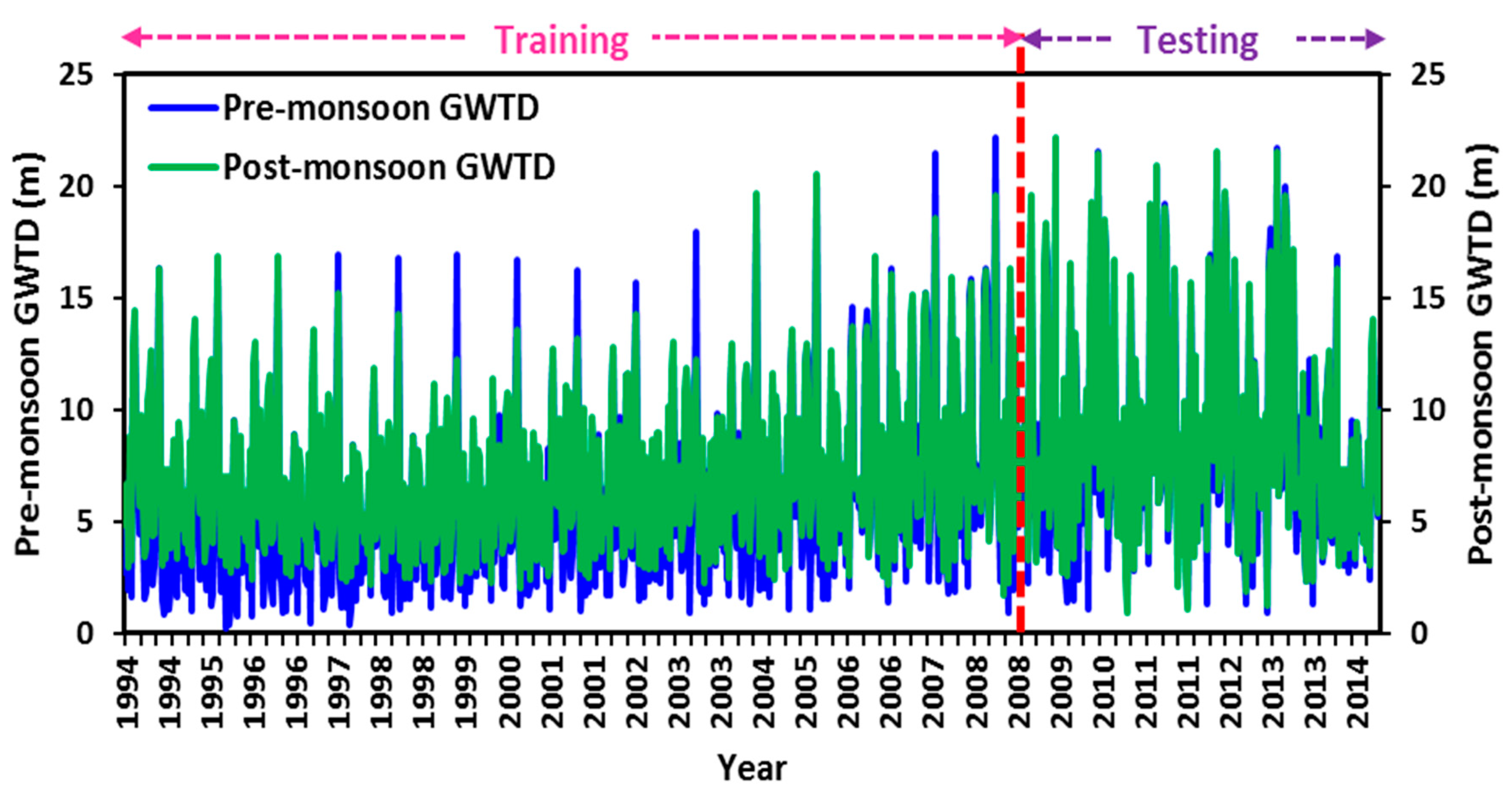
2.2. Hydrogeology of Study Area and Data Acquisition
- Aquifer type group I is composed of different types of basalt rocks, like weathered, dense, and vesicular. Groundwater occurs under water table conditions 30 m or lower than ground level. The tube well discharge varies from 97 to 227 m3/h for drawdown between 2.68 m and 0.68 m.
- Aquifer type group II is mainly sandstone, siltstone, limestone, and schist. The piezometric head of the horizontal flowing wells lies between 6.63 and 8.92 m above the groundwater level. In the non-flowing wells, it ranges between 1.55 and 11.34 m below the ground level. Most tube wells constructed in this region register a free flow, ranging from 80 to 210 m3/h. In the non-flowing wells, the discharge head varies from 2 to 8 m.
- Aquifer type group III is composed of gravel, pebbles, grit, sand, clay, etc. Quaternary aquifers belong to this group. Groundwater occurs under unconfined conditions in surface or near-surface aquifers. Water depth varies from 0.2 to 9.7 m.
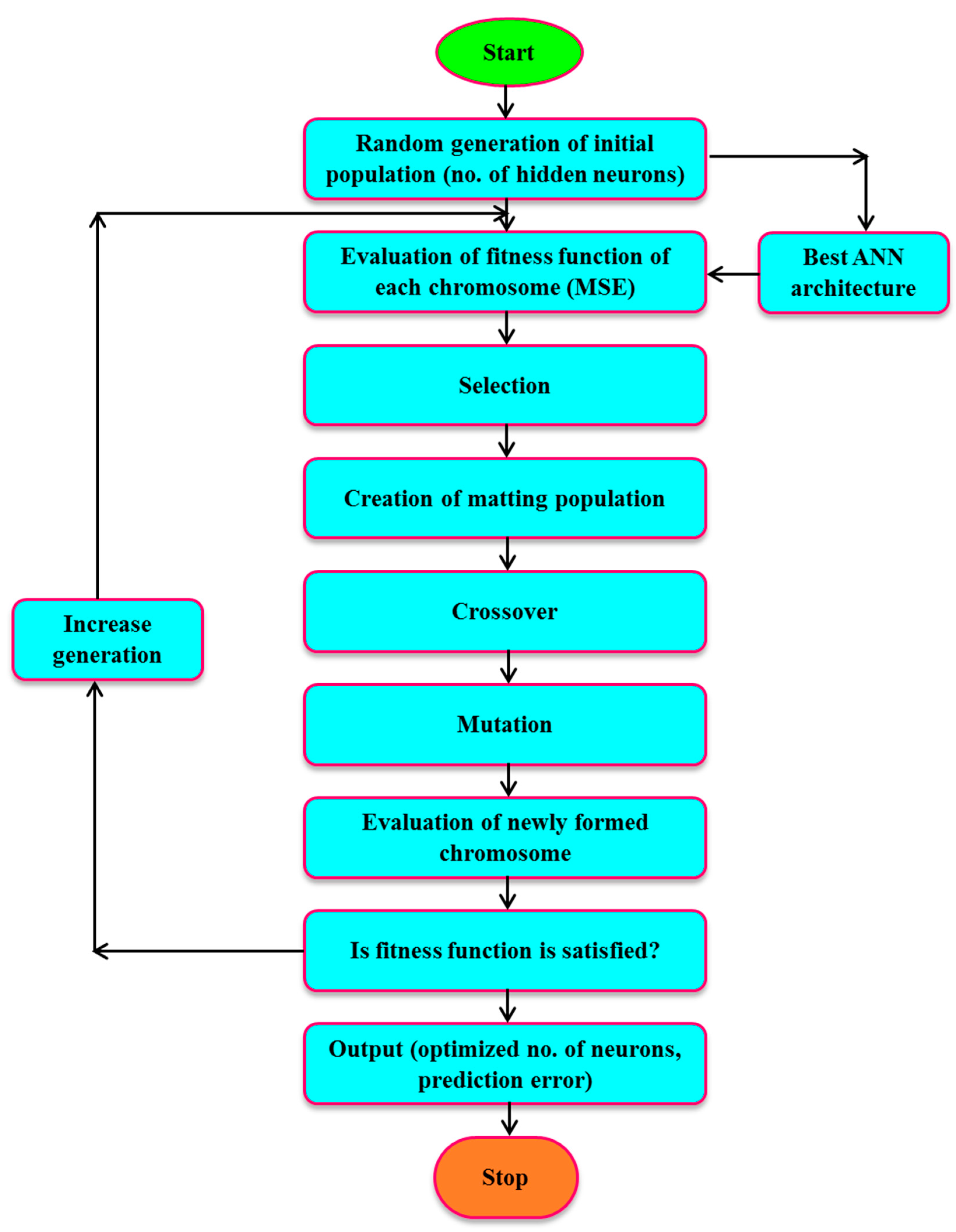
2.3. Genetic Algorithm (GA)
- Start: Generate chromosomes by random population.
- Fitness: Determine the fitness function in the populations of every chromosome.
- New Population: Develop the new population by following the steps that follow until completing the new population.
- (a)
- Selection: Based on their fitness, identify two parent chromosomes from a population.
- (b)
- Crossover: Cross the parents to create a new spring (children), with the possibility of a crossover. When there is no crossover, offspring are the exact duplicate of the parents.
- (c)
- Mutation: Mutate new offspring at each locus, with the likelihood of mutation.
- (d)
- Accepting: In the new population, locate new offspring.
- Replace: For the further running of the algorithm, use the newly created population.
- Test: When the ended conditions are encountered, the current population’s best outcome will stop and return.
- Loop: Switch back to Step 2.
2.4. Hybrid Genetic Algorithm-Artificial Neural Network (GA-ANN)
- The GA technique is used to improve the topology of the ANN and its variables.
- The optimal response is obtained using ANN.
2.5. Determination of the Parameters the ANN Model
2.6. Development of GA-ANN and GA Models for GWTD Prediction
2.7. Statistical Indicators
3. Results and Discussion
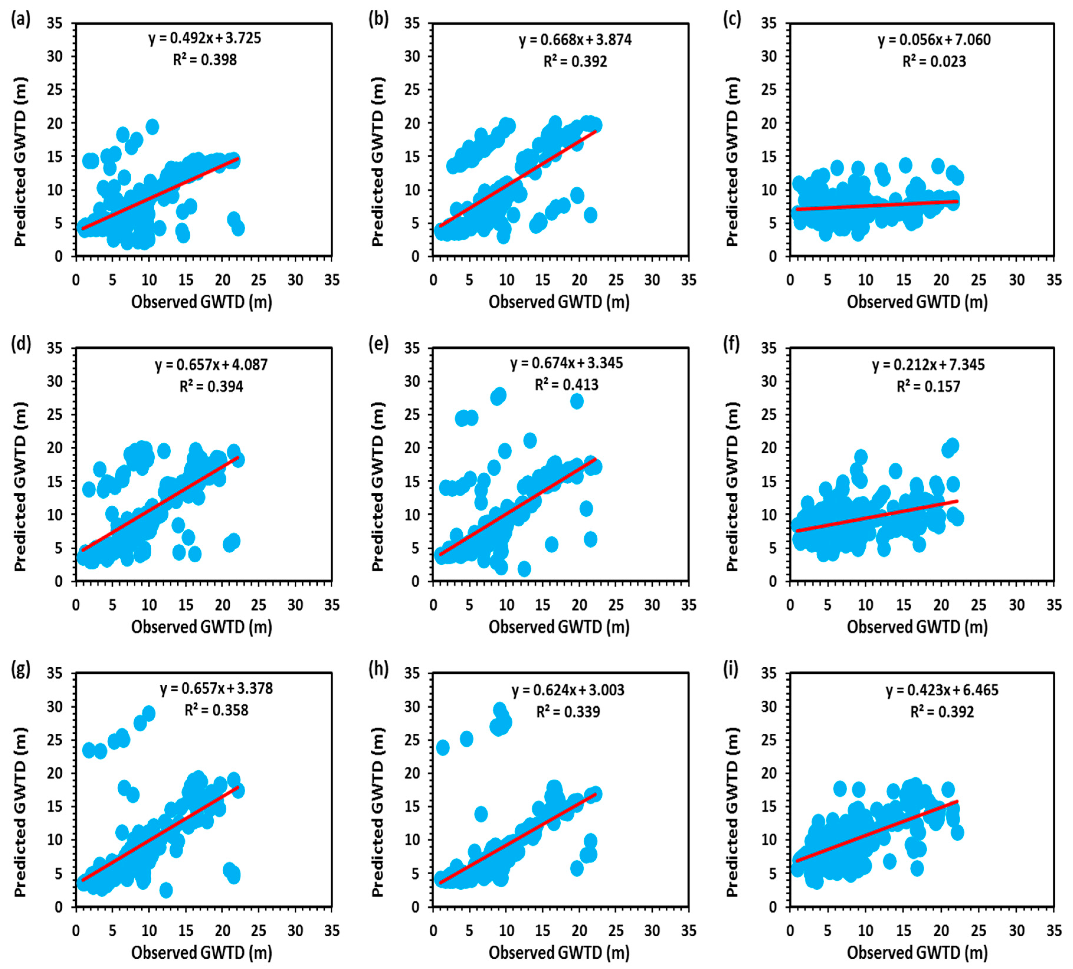
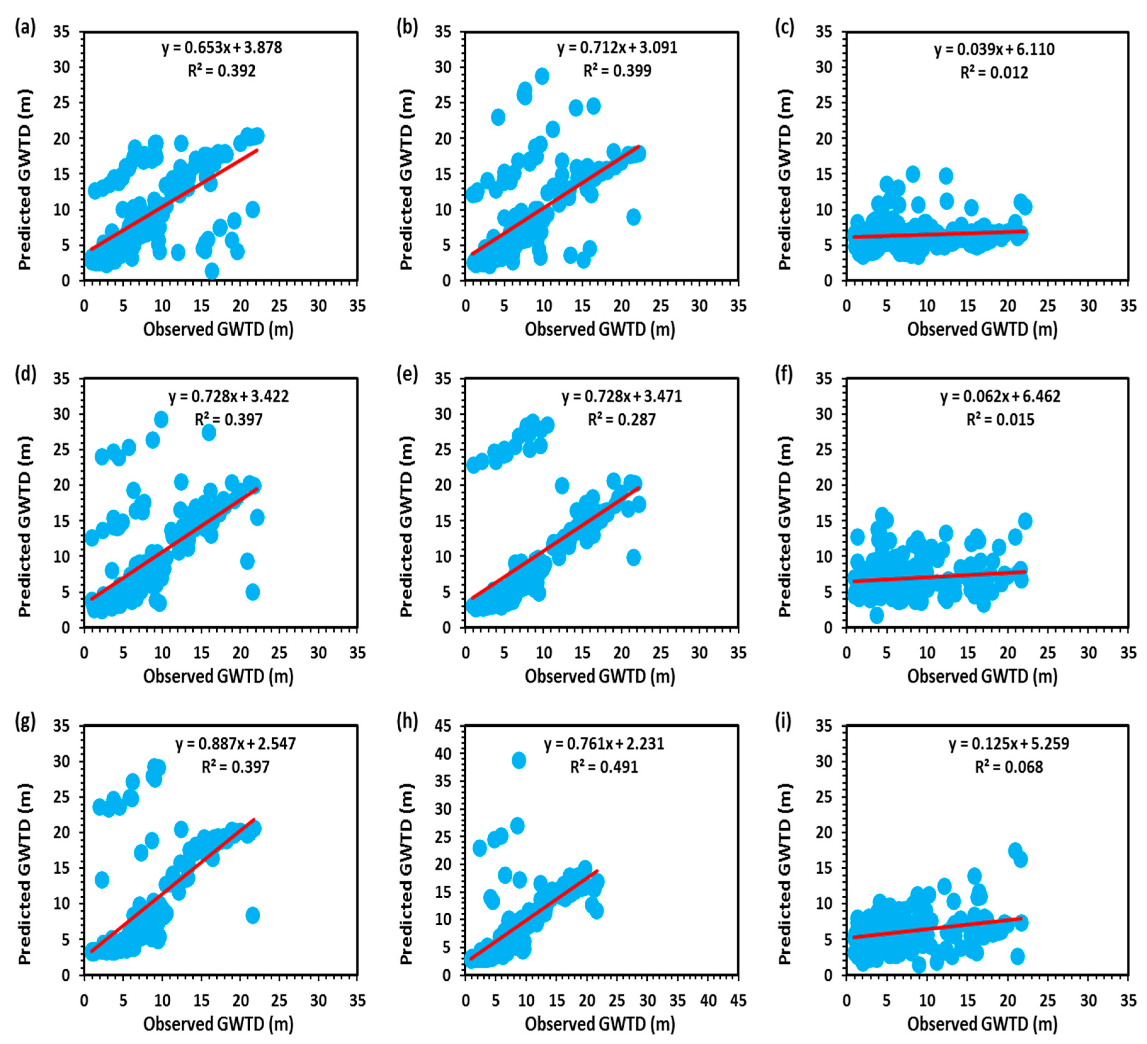
3.1. Prediction of GWTD Using Traditional GA Method
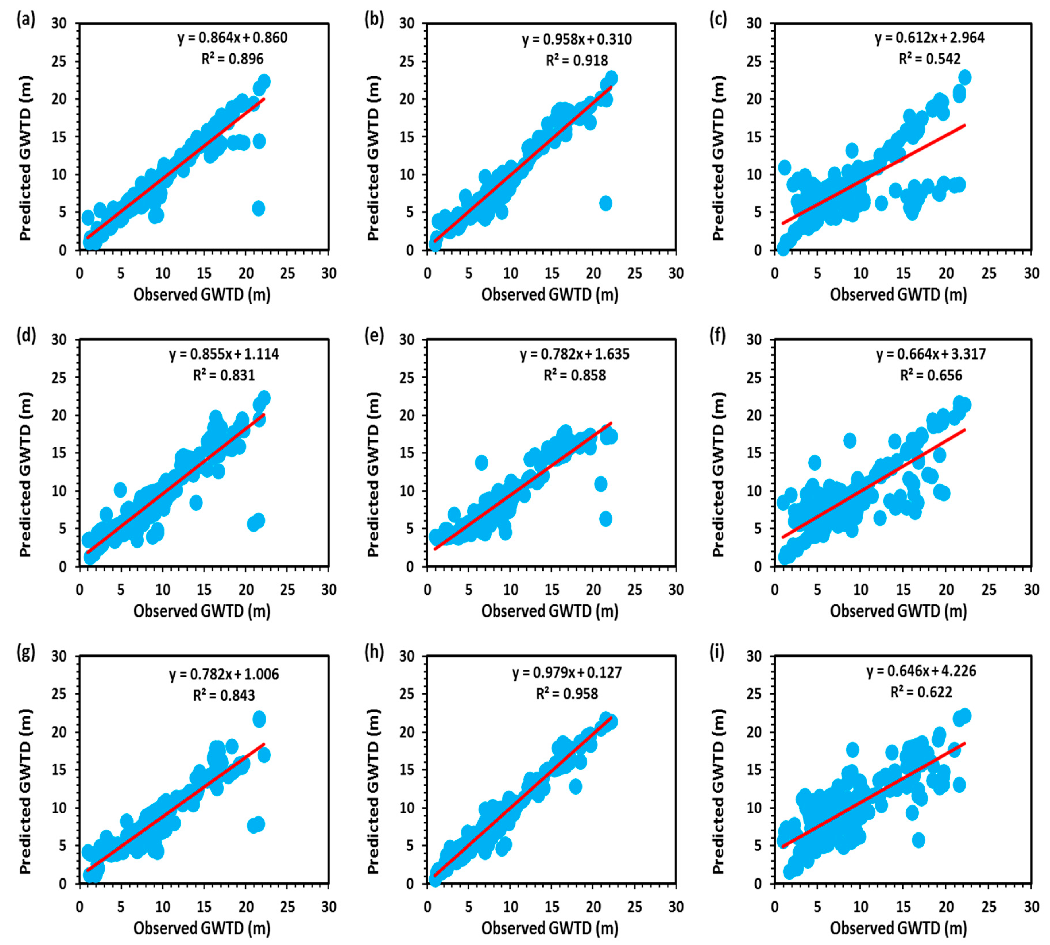
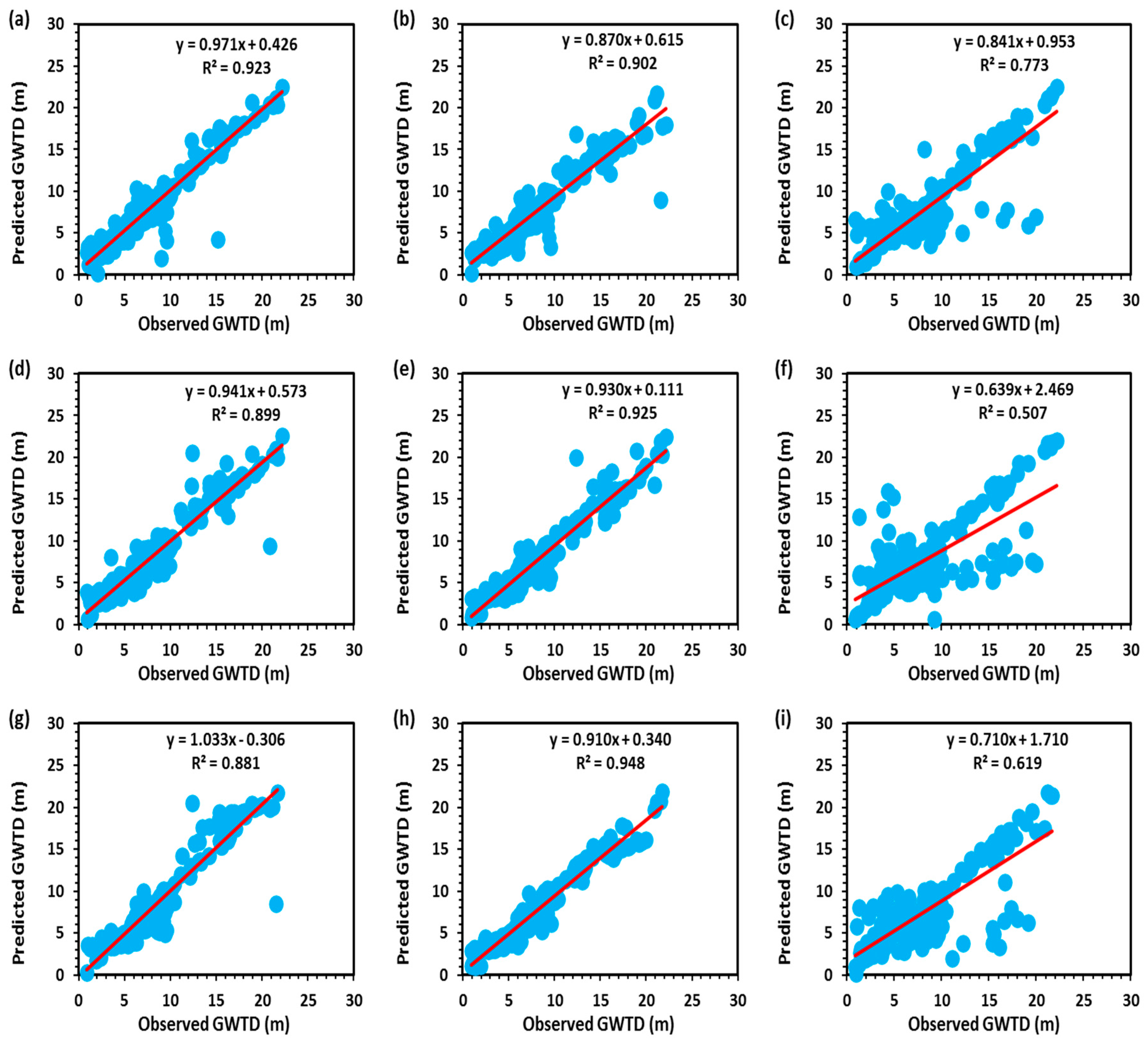
3.2. Prediction of GWTD Using GA-ANN Models
4. Conclusions
Author Contributions
Funding
Conflicts of Interest
References
- Nunno, F.D.; Granata, F. Groundwater level prediction in Apulia region (Southern Italy) using NARX neural network. Environ. Res. 2020, 190, 110062. [Google Scholar] [PubMed]
- Amarasinghe, U.A.; Smakhtin, V. Global water demand projections: Past, present and future. Int. Water Manag. Inst. (IWMI) Colombo Sri Lanka 2014, 156, 1–24. [Google Scholar]
- Haas, J.C.; Birk, S. Characterizing the spatiotemporal variability of groundwater levels of alluvial aquifers in different settings using drought indices. Hydrol. Earth Syst. Sci. 2017, 21, 2421–2448. [Google Scholar] [CrossRef]
- Yu, H.; Wen, X.; Feng, Q.; Deo, R.C.; Si, J.; Wu, M. Comparative Study of Hybrid-Wavelet Artificial Intelligence Models for Monthly Groundwater Depth Forecasting in Extreme Arid Regions, Northwest China. Water Resour. Manag. 2018, 32, 301–323. [Google Scholar] [CrossRef]
- Goldman, M.; Neubauer, F.M. Groundwater exploration using integrated geophysical techniques. Surv. Geophys. 1994, 15, 331–361. [Google Scholar] [CrossRef]
- Singh, A.; Malik, A.; Kumar, A.; Kisi, O. Rainfall-runoff modeling in hilly watershed using heuristic approaches with gamma test. Arab. J. Geosci. 2018, 11, 1–12. [Google Scholar] [CrossRef]
- Malik, A.; Tikhamarine, Y.; Souag-Gamane, D.; Kisi, O.; Pham, Q.B. Support vector regression optimized by meta-heuristic algorithms for daily streamflow prediction. Stoch. Environ. Res. Risk Assess. 2020. [Google Scholar] [CrossRef]
- Tikhamarine, Y.; Souag-Gamane, D.; Ahmed, A.N.; Sammen, S.S.; Kisi, O.; Huang, Y.F.; El-Shafie, A. Rainfall-runoff modelling using improved machine learning methods: Harris hawks optimizer vs. particle swarm optimization. J. Hydrol. 2020, 589, 125133. [Google Scholar] [CrossRef]
- Malik, A.; Kumar, A.; Singh, R.P. Application of Heuristic Approaches for Prediction of Hydrological Drought Using Multi-scalar Streamflow Drought Index. Water Resour. Manag. 2019, 33, 3985–4006. [Google Scholar] [CrossRef]
- Malik, A.; Kumar, A. Meteorological drought prediction using heuristic approaches based on effective drought index: A case study in Uttarakhand. Arab. J. Geosci. 2020, 13, 1–17. [Google Scholar] [CrossRef]
- Malik, A.; Kumar, A.; Salih, S.Q.; Kim, S.; Kim, N.W.; Yaseen, Z.M.; Singh, V.P. Drought index prediction using advanced fuzzy logic model: Regional case study over Kumaon in India. PLoS ONE 2020, 15, e0233280. [Google Scholar] [CrossRef] [PubMed]
- Malik, A.; Kumar, A.; Kisi, O. Monthly pan-evaporation estimation in Indian central Himalayas using different heuristic approaches and climate based models. Comput. Electron. Agric. 2017, 143, 302–313. [Google Scholar] [CrossRef]
- Malik, A.; Kumar, A.; Kisi, O. Daily Pan Evaporation Estimation Using Heuristic Methods with Gamma Test. J. Irrig. Drain. Eng. 2018, 144, 04018023. [Google Scholar] [CrossRef]
- Malik, A.; Rai, P.; Heddam, S.; Kisi, O.; Sharafati, A.; Salih, S.Q.; Al-Ansari, N.; Yaseen, Z.M. Pan Evaporation Estimation in Uttarakhand and Uttar Pradesh States, India: Validity of an Integrative Data Intelligence Model. Atmosphere 2020, 11, 553. [Google Scholar] [CrossRef]
- Malik, A.; Kumar, A.; Kim, S.; Kashani, M.H.; Karimi, V.; Sharafati, A.; Ghorbani, M.A.; Al-Ansari, N.; Salih, S.Q.; Yaseen, Z.M.; et al. Modeling monthly pan evaporation process over the Indian central Himalayas: Application of multiple learning artificial intelligence model. Eng. Appl. Comput. Fluid Mech. 2020, 14, 323–338. [Google Scholar] [CrossRef]
- Malik, A.; Kumar, A.; Ghorbani, M.A.; Kashani, M.H.; Kisi, O.; Kim, S. The viability of co-active fuzzy inference system model for monthly reference evapotranspiration estimation: Case study of Uttarakhand State. Hydrol. Res. 2019, 50, 1623–1644. [Google Scholar] [CrossRef]
- Tikhamarine, Y.; Malik, A.; Kumar, A.; Souag-Gamane, D.; Kisi, O. Estimation of monthly reference evapotranspiration using novel hybrid machine learning approaches. Hydrol. Sci. J. 2019, 64, 1824–1842. [Google Scholar] [CrossRef]
- Tikhamarine, Y.; Malik, A.; Souag-Gamane, D.; Kisi, O. Artificial intelligence models versus empirical equations for modeling monthly reference evapotranspiration. Environ. Sci. Pollut. Res. 2020, 27, 30001–30019. [Google Scholar] [CrossRef]
- Huang, X.; Gao, L.; Crosbie, R.S.; Zhang, N.; Fu, G.; Doble, R. Groundwater Recharge Prediction Using Linear Regression, Multi-Layer Perception Network, and Deep Learning. Water 2019, 11, 1879. [Google Scholar] [CrossRef]
- Chen, L.-H.; Chen, C.-T.; Pan, Y.-G. Groundwater Level Prediction Using SOM-RBFN Multisite Model. J. Hydrol. Eng. 2010, 15, 624–631. [Google Scholar] [CrossRef]
- Chen, L.-H.; Chen, C.-T.; Lin, D.-W. Application of Integrated Back-Propagation Network and Self-Organizing Map for Groundwater Level Forecasting. J. Water Resour. Plan. Manag. 2011, 137, 352–365. [Google Scholar] [CrossRef]
- Panahi, M.; Sadhasivam, N.; Pourghasemi, H.R.; Rezaie, F.; Lee, S. Spatial prediction of groundwater potential mapping based on convolutional neural network (CNN) and support vector regression (SVR). J. Hydrol. 2020, 588, 125033. [Google Scholar] [CrossRef]
- Gong, Y.; Zhang, Y.; Lan, S.; Wang, H. A Comparative Study of Artificial Neural Networks, Support Vector Machines and Adaptive Neuro Fuzzy Inference System for Forecasting Groundwater Levels near Lake Okeechobee, Florida. Water Resour. Manag. 2016, 30, 375–391. [Google Scholar] [CrossRef]
- Arabameri, A.; Lee, S.; Tiefenbacher, J.P.; Ngo, P.T.T. Novel Ensemble of MCDM-Artificial Intelligence Techniques for Groundwater-Potential Mapping in Arid and Semi-Arid Regions (Iran). Remote Sens. 2020, 12, 490. [Google Scholar] [CrossRef]
- Natarajan, N.; Sudheer, C. Groundwater level forecasting using soft computing techniques. Neural Comput. Appl. 2020, 32, 7691–7708. [Google Scholar] [CrossRef]
- Pradhan, S.; Kumar, S.; Kumar, Y.; Sharma, H.C. Assessment of groundwater utilization status and prediction of water table depth using different heuristic models in an Indian interbasin. Soft Comput. 2019, 23, 10261–10285. [Google Scholar] [CrossRef]
- Deb, P.; Kiem, A.S.; Willgoose, G. A linked surface water-groundwater modelling approach to more realistically simulate rainfall-runoff non-stationarity in semi-arid regions. J. Hydrol. 2019, 575, 273–291. [Google Scholar] [CrossRef]
- Deb, P.; Kiem, A.S. Evaluation of rainfall–runoff model performance under non-stationary hydroclimatic conditions. Hydrol. Sci. J. 2020, 65, 1667–1684. [Google Scholar] [CrossRef]
- Tayyab, M.; Zhou, J.; Zeng, X.; Adnan, R. Discharge Forecasting By Applying Artificial Neural Networks At The Jinsha River Basin, China. Eur. Sci. J. ESJ 2016, 12, 108. [Google Scholar] [CrossRef][Green Version]
- Khan, M.Y.A.; Hasan, F.; Panwar, S.; Chakrapani, G.J. Neural network model for discharge and water-level prediction for Ramganga River catchment of Ganga Basin, India. Hydrol. Sci. J. 2016, 61, 2084–2095. [Google Scholar] [CrossRef]
- Zhou, T.; Wang, F.; Yang, Z. Comparative Analysis of ANN and SVM Models Combined with Wavelet Preprocess for Groundwater Depth Prediction. Water 2017, 9, 781. [Google Scholar] [CrossRef]
- Muhammad, R.; Yuan, X.; Kisi, O.; Yuan, Y. Streamflow Forecasting Using Artificial Neural Network and Support Vector Machine Models. Am. Sci. Res. J. Eng. Technol. Sci. 2017, 29, 286–294. [Google Scholar]
- Gaur, S.; Ch, S.; Graillot, D.; Chahar, B.R.; Kumar, D.N. Application of Artificial Neural Networks and Particle Swarm Optimization for the Management of Groundwater Resources. Water Resour. Manag. 2013, 27, 927–941. [Google Scholar] [CrossRef]
- Alizamir, M.; Sobhanardakani, S. An Artificial Neural Network - Particle Swarm Optimization (ANN- PSO) Approach to Predict Heavy Metals Contamination in Groundwater Resources. Jundishapur J. Health Sci. 2018, 10, e67544. [Google Scholar] [CrossRef]
- Afzaal, H.; Farooque, A.A.; Abbas, F.; Acharya, B.; Esau, T. Groundwater Estimation from Major Physical Hydrology Components Using Artificial Neural Networks and Deep Learning. Water 2019, 12, 5. [Google Scholar] [CrossRef]
- Cho, K.H.; Sthiannopkao, S.; Pachepsky, Y.A.; Kim, K.-W.; Kim, J.H. Prediction of contamination potential of groundwater arsenic in Cambodia, Laos, and Thailand using artificial neural network. Water Res. 2011, 45, 5535–5544. [Google Scholar] [CrossRef] [PubMed]
- Wagh, V.M.; Panaskar, D.B.; Muley, A.A.; Mukate, S.V.; Lolage, Y.P.; Aamalawar, M.L. Prediction of groundwater suitability for irrigation using artificial neural network model: A case study of Nanded tehsil, Maharashtra, India. Model. Earth Syst. Environ. 2016, 2, 1–10. [Google Scholar] [CrossRef]
- Chen, S.; Fang, G.; Huang, X.; Zhang, Y. Water Quality Prediction Model of a Water Diversion Project Based on the Improved Artificial Bee Colony–Backpropagation Neural Network. Water 2018, 10, 806. [Google Scholar] [CrossRef]
- Azimi, S.; Azhdary Moghaddam, M.; Hashemi Monfared, S.A. Prediction of annual drinking water quality reduction based on Groundwater Resource Index using the artificial neural network and fuzzy clustering. J. Contam. Hydrol. 2019, 220, 6–17. [Google Scholar] [CrossRef]
- Das, A.; Maiti, S.; Naidu, S.; Gupta, G. Estimation of spatial variability of aquifer parameters from geophysical methods: A case study of Sindhudurg district, Maharashtra, India. Stoch. Environ. Res. Risk Assess. 2017, 31, 1709–1726. [Google Scholar] [CrossRef]
- Thomas, A.; Eldho, T.I.; Rastogi, A.K.; Majumder, P. A comparative study in aquifer parameter estimation using MFree point collocation method with evolutionary algorithms. J. Hydroinform. 2019, 21, 455–473. [Google Scholar] [CrossRef]
- Delnaz, A.; Rakhshandehroo, G.; Nikoo, M.R. Confined Aquifer’s Hydraulic Parameters Estimation by a Generalized Regression Neural Network. Iran. J. Sci. Technol. Trans. Civ. Eng. 2020, 44, 259–269. [Google Scholar] [CrossRef]
- Mohanty, S.; Jha, M.K.; Kumar, A.; Sudheer, K.P. Artificial Neural Network Modeling for Groundwater Level Forecasting in a River Island of Eastern India. Water Resour. Manag. 2010, 24, 1845–1865. [Google Scholar] [CrossRef]
- Jha, M.K.; Sahoo, S. Efficacy of neural network and genetic algorithm techniques in simulating spatio-temporal fluctuations of groundwater. Hydrol. Process. 2015, 29, 671–691. [Google Scholar] [CrossRef]
- Nourani, V.; Ejlali, R.G.; Alami, M.T. Spatiotemporal Groundwater Level Forecasting in Coastal Aquifers by Hybrid Artificial Neural Network-Geostatistics Model: A Case Study. Environ. Eng. Sci. 2011, 28, 217–228. [Google Scholar] [CrossRef]
- Chitsazan, M.; Rahmani, G.; Neyamadpour, A. Forecasting groundwater level by artificial neural networks as an alternative approach to groundwater modeling. J. Geol. Soc. India 2015, 85, 98–106. [Google Scholar] [CrossRef]
- Van Ty, T.; Van Phat, L.; Van Hiep, H. Groundwater Level Prediction Using Artificial Neural Networks: A Case Study in Tra Noc Industrial Zone, Can Tho City, Vietnam. J. Water Resour. Prot. 2018, 10, 870–883. [Google Scholar] [CrossRef][Green Version]
- Chang, J.; Wang, G.; Mao, T. Simulation and prediction of suprapermafrost groundwater level variation in response to climate change using a neural network model. J. Hydrol. 2015, 529, 1211–1220. [Google Scholar] [CrossRef]
- Banadkooki, F.B.; Ehteram, M.; Ahmed, A.N.; Teo, F.Y.; Fai, C.M.; Afan, H.A.; Sapitang, M.; El-Shafie, A. Enhancement of Groundwater-Level Prediction Using an Integrated Machine Learning Model Optimized by Whale Algorithm. Nat. Resour. Res. 2020, 29, 3233–3252. [Google Scholar] [CrossRef]
- Majumder, P.; Eldho, T.I. Artificial Neural Network and Grey Wolf Optimizer Based Surrogate Simulation-Optimization Model for Groundwater Remediation. Water Resour. Manag. 2020, 34, 763–783. [Google Scholar] [CrossRef]
- Mohanty, S.; Jha, M.K.; Raul, S.K.; Panda, R.K.; Sudheer, K.P. Using Artificial Neural Network Approach for Simultaneous Forecasting of Weekly Groundwater Levels at Multiple Sites. Water Resour. Manag. 2015, 29, 5521–5532. [Google Scholar] [CrossRef]
- Shiri, J.; Kisi, O.; Yoon, H.; Lee, K.-K.; Hossein Nazemi, A. Predicting groundwater level fluctuations with meteorological effect implications—A comparative study among soft computing techniques. Comput. Geosci. 2013, 56, 32–44. [Google Scholar] [CrossRef]
- Kisi, O.; Yaseen, Z.M. The potential of hybrid evolutionary fuzzy intelligence model for suspended sediment concentration prediction. Catena 2019, 174, 11–23. [Google Scholar] [CrossRef]
- Tikhamarine, Y.; Souag-Gamane, D.; Najah Ahmed, A.; Kisi, O.; El-Shafie, A. Improving artificial intelligence models accuracy for monthly streamflow forecasting using grey Wolf optimization (GWO) algorithm. J. Hydrol. 2020, 582, 124435. [Google Scholar] [CrossRef]
- Tikhamarine, Y.; Souag-Gamane, D.; Kisi, O. A new intelligent method for monthly streamflow prediction: Hybrid wavelet support vector regression based on grey wolf optimizer (WSVR–GWO). Arab. J. Geosci. 2019, 12, 540. [Google Scholar] [CrossRef]
- Singh, R.M.; Datta, B. Identification of Groundwater Pollution Sources Using GA-based Linked Simulation Optimization Model. J. Hydrol. Eng. 2006, 11, 101–109. [Google Scholar] [CrossRef]
- Jain, A.; Bhattacharjya, R.K.; Sanaga, S. Optimal Design of Composite Channels Using Genetic Algorithm. J. Irrig. Drain. Eng. 2004, 130, 286–295. [Google Scholar] [CrossRef]
- Şen, Z.; Öztopal, A. Genetic algorithms for the classification and prediction of precipitation occurrence. Hydrol. Sci. J. 2001, 46, 255–267. [Google Scholar] [CrossRef]
- Ni, Q.; Wang, L.; Zheng, B.; Sivakumar, M. Evolutionary Algorithm for Water Storage Forecasting Response to Climate Change with Small Data Sets: The Wolonghu Wetland, China. Environ. Eng. Sci. 2012, 29, 814–820. [Google Scholar] [CrossRef]
- Aytek, A.; Kişi, Ö. A genetic programming approach to suspended sediment modelling. J. Hydrol. 2008, 351, 288–298. [Google Scholar] [CrossRef]
- Jalalkamali, A.; Sedghi, H.; Manshouri, M. Monthly groundwater level prediction using ANN and neuro-fuzzy models: A case study on Kerman plain, Iran. J. Hydroinform. 2011, 13, 867–876. [Google Scholar] [CrossRef]
- Dash, N.B.; Panda, S.N.; Remesan, R.; Sahoo, N. Hybrid neural modeling for groundwater level prediction. Neural Comput. Appl. 2010, 19, 1251–1263. [Google Scholar] [CrossRef]
- Supreetha, B.S.; Prabhakar Nayak, K.; Narayan Shenoy, K. Groundwater level prediction using hybrid artificial neural network with genetic algorithm. Int. J. Earth Sci. Eng. 2015, 8, 2609–2615. [Google Scholar]
- Hosseini, Z.; Nakhaie, M. Estimation of groundwater level using a hybrid genetic algorithm-neural network. Pollution 2015, 1, 9–21. [Google Scholar]
- Jalalkamali, A. Groundwater modeling using hybrid of artificial neural network with genetic algorithm. Afr. J. Agric. Res. 2011, 6, 5775–5784. [Google Scholar] [CrossRef]
- Roshni, T.; Jha, M.K.; Drisya, J. Neural network modeling for groundwater-level forecasting in coastal aquifers. Neural Comput. Appl. 2020, 32, 12737–12754. [Google Scholar] [CrossRef]
- Karamouz, M.; Tabari, M.M.R.; Kerachian, R. Application of Genetic Algorithms and Artificial Neural Networks in Conjunctive Use of Surface and Groundwater Resources. Water Int. 2007, 32, 163–176. [Google Scholar] [CrossRef]
- Wibowo, A.; Arbain, S.H.; Abidin, N.Z. Combined multiple neural networks and genetic algorithm with missing data treatment: Case study of water level forecasting in Dungun River—Malaysia. IAENG Int. J. Comput. Sci. 2018, 45, 1–9. [Google Scholar]
- Li, H.; Lu, Y.; Zheng, C.; Yang, M.; Li, S. Groundwater Level Prediction for the Arid Oasis of Northwest China Based on the Artificial Bee Colony Algorithm and a Back-propagation Neural Network with Double Hidden Layers. Water 2019, 11, 860. [Google Scholar] [CrossRef]
- CGWB. Status Report on Review of Ground Water Resources Estimation Methodology; Central Ground Water Board: Faridabad, India, 2009; pp. 1–66. [Google Scholar]
- Goldberg, D.E. Genetic Algorithms in Search, Optimization, and Machine Learning; Addison Wesley, Reading: Boston, MA, USA, 1989. [Google Scholar]
- Malhotra, R.; Singh, N.; Singh, Y. Genetic Algorithms: Concepts, Design for Optimization of Process Controllers. Comput. Inf. Sci. 2011, 4, 39–54. [Google Scholar] [CrossRef]
- Chang, Y.-T.; Lin, J.; Shieh, J.-S.; Abbod, M.F. Optimization the Initial Weights of Artificial Neural Networks via Genetic Algorithm Applied to Hip Bone Fracture Prediction. Adv. Fuzzy Syst. 2012, 2012, 1–9. [Google Scholar] [CrossRef]
- Tahmasebi, P.; Hezarkhani, A. A hybrid neural networks-fuzzy logic-genetic algorithm for grade estimation. Comput. Geosci. 2012, 42, 18–27. [Google Scholar] [CrossRef]
- Mattioli, F.; Caetano, D.; Cardoso, A.; Naves, E.; Lamounier, E. An Experiment on the Use of Genetic Algorithms for Topology Selection in Deep Learning. J. Electr. Comput. Eng. 2019, 2019, 1–12. [Google Scholar] [CrossRef]
- Castillo, P.A.; Merelo, J.J.; Prieto, A.; Rivas, V.; Romero, G. G-Prop: Global optimization of multilayer perceptrons using GAs. Neurocomputing 2000, 35, 149–163. [Google Scholar] [CrossRef]
- Gerken, W.C.; Purvis, L.K.; Butera, R.J. Genetic algorithm for optimization and specification of a neuron model. Neurocomputing 2006, 69, 1039–1042. [Google Scholar] [CrossRef]
- MWRI. Report of the Ground Water Resource Estimation Committee; Ministry of Water Resources: New Delhi, India, 2009; p. 133.
- Chandra, S. Estimation and measurement of recharge to groundwater from rainfall, irrigation and influent seepage. In Proceedings of the International Seminar on Development and Management of Groundwater Resources, Roorkee, India, 5–20 November 1979; pp. 9–17. [Google Scholar]
- ARDC. Report of Ground Water over Exploitation Committee; Agricultural Refinance and Development Corporation: Mumbai, Indian, 1979; pp. 211–232. [Google Scholar]
- Adnan, R.M.; Malik, A.; Kumar, A.; Parmar, K.S.; Kisi, O. Pan evaporation modeling by three different neuro-fuzzy intelligent systems using climatic inputs. Arab. J. Geosci. 2019, 12, 606. [Google Scholar] [CrossRef]
- Coulibaly, P.; Anctil, F.; Aravena, R.; Bobée, B. Artificial neural network modeling of water table depth fluctuations. Water Resour. Res. 2001, 37, 885–896. [Google Scholar] [CrossRef]
- Das, U.K.; Roy, P.; Ghose, D.K. Modeling water table depth using adaptive Neuro-Fuzzy Inference System. ISH J. Hydraul. Eng. 2019, 25, 291–297. [Google Scholar] [CrossRef]
- Shiri, J.; Kisi, O.; Yoon, H.; Kazemi, M.H.; Shiri, N.; Poorrajabali, M.; Karimi, S. Prediction of groundwater level variations in coastal aquifers with tide and rainfall effects using heuristic data driven models. ISH J. Hydraul. Eng. 2020, 26, 1–11. [Google Scholar] [CrossRef]
- Cai, X.; McKinney, D.C.; Lasdon, L.S. Solving nonlinear water management models using a combined genetic algorithm and linear programming approach. Adv. Water Resour. 2001, 24, 667–676. [Google Scholar] [CrossRef]
- Chiu, Y.-C.; Chang, L.-C.; Chang, F.-J. Using a hybrid genetic algorithm–simulated annealing algorithm for fuzzy programming of reservoir operation. Hydrol. Process. 2007, 21, 3162–3172. [Google Scholar] [CrossRef]
- Sharafati, A.; Tafarojnoruz, A.; Shourian, M.; Yaseen, Z.M. Simulation of the depth scouring downstream sluice gate: The validation of newly developed data-intelligent models. J. Hydro-Environ. Res. 2020, 29, 20–30. [Google Scholar] [CrossRef]


| GA Parameter | Type/Value |
|---|---|
| Population size | 50 |
| Population type | Double vector |
| Population initial range | [3 × 1double] |
| Selection Mechanism | Roulette wheel |
| Basis of chromosome selection | Fitness function (MSE) |
| Crossover type | Double |
| Crossover Probability | 0.8–1.0 |
| Mutation type | Gaussian |
| Mutation Probability | 0.001–0.01 |
| Elite count | 2 |
| Migration direction | Forward |
| Migration interval | 20 |
| Time limit | Infinite |
| Stall Generation limit | Inf |
| Maximum number of generations | 100 |
| Termination Criteria | 0.001 m2 |
| Display | Iteration |
| Model | Output | Input |
|---|---|---|
| Pre-monsoon season | ||
| 1 | WTpr | F[(ms,n−1) + (Nms,n−1 to n), (ms,n−1) + (Nms,n−1 to n), WTpr,n−1] |
| 2 | WTpr | F[(ms,n−1) + (Nms,n−1 to n), (ms,n−1) + (Nms,n−1 to n), WTpr,n−1, WTps,n−1] |
| 3 | WTpr | F[(ms,n−1) + (Nms,n−1 to n), (ms,n−1) + (Nms,n−1 to n), ∆WT(pr,n−1–ps,n−1) ] |
| 4 | WTpr | F[(Nms,n−1 to n) + (ms,n−1) + (Nms,n−2 to n−1) + (ms,n−2),(Nms,n−1 to n) + (ms,n−1) + (Nms,n−2 to n−1) + (ms,n−2), WTpr,n−2] |
| 5 | WTpr | F[(Nms,n−1 to n) + (ms,n−1) + (Nms,n−2 to n−1) + (ms,n−2), (Nms,n−1 to n) + (ms,n−1) + (Nms,n−2 to n−1) + (ms,n−2), WTpr,n−2, WTps,n−2, WTpr,n−1, WTps,n−1] |
| 6 | WTpr | F[(Nms,n−1 to n) + (ms,n−1) + (Nms,n−2 to n−1) + (ms,n−2), (Nms,n−1 to n) + (ms,n−1) + (Nms,n−2 to n−1) + (ms,n−2), ∆WT(pr,n−2–ps,n−2), ∆WT(ps,n−2–pr,n−1), ∆WT(pr,n−1–ps,n−1)] |
| 7 | WTpr | F[(Nms,n−1 to n) + (ms,n−1) + (Nms,n−2 to n−1) + (ms,n−2) + (Nms,n−3 to n−2) + (ms,n−3), (Nms,n−1 to n) + (ms,n−1) + (Nms,n−2 to n−1) + (ms,n−2) + (Nms,n−3 to n−2) + (ms,n−3), WTpr,n−3] |
| 8 | WTpr | F[(Nms,n−1 to n) + (ms,n−1) + (Nms,n−2 to n−1) + (ms,n−2) + (Nms,n−3 to n−2) + (ms,n−3), (Nms,n−1 to n) + (ms,n−1) + (Nms,n−2 to n−1) + (ms,n−2) + (Nms,n−3 to n−2) + (ms,n−3), WTpr,n−3, WTps,n−3, WTpr,n−2, WTps,n−2, WTpr,n−1, WTps,n−1] |
| 9 | WTpr | F[(Nms,n−1 to n) + (ms,n−1) + (Nms,n−2 to n−1) + (ms,n−2) + (Nms,n−3 to n−2) + (ms,n−3),(Nms,n−1 to n) + (ms,n−1) + (Nms,n−2 to n−1) + (ms,n−2) + (Nms,n−3 to n−2) + (ms,n−3), ∆WT(pr,n−3–ps,n−3), ∆WT(ps,n−3–pr,n−2), ∆WT(pr,n−2–ps,n−2), ∆WT(ps,n−2–pr,n−1), ∆WT(pr,n−1–ps,n−1)] |
| Post-monsoon season | ||
| 1 | WTps | F[(ms,n) + (Nms,n−1 to n), (ms,n) + (Nms,n−1 to n), WTps,n−1] |
| 2 | WTps | F[(ms,n) + (Nms,n−1 to n), (ms,n) + (Nms,n−1 to n), WTps,n−1, WTpr,n] |
| 3 | WTps | F[(ms,n) + (Nms,n−1 to n), (ms,n) + (Nms,n−1 to n), ∆WT(ps,n−1–pr,n)] |
| 4 | WTps | F[(ms,n) + (Nms,n−1 to n) + (ms,n−1) + (Nms,n−1 to n−2), (ms,n) + (Nms,n−1 to n) + (ms,n−1) + (Nms,n−1 to n−2), WTps,n−2] |
| 5 | WTps | F[(ms,n) + (Nms,n−1 to n) + (ms,n−1) + (Nms,n−1 to n−2), (ms,n) + (Nms,n−1 to n) + (ms,n−1) + (Nms,n−1 to n−2), WTps,n−2, WTpr,n−1, WTps,n−1, WTpr,n] |
| 6 | WTps | F[(ms,n) + (Nms,n−1 to n) + (ms,n−1) + (Nms,n−1 to n−2), (ms,n) + (Nms,n−1 to n) + (ms,n−1) + (Nms,n−1 to n−2), ∆WT(ps,n−2–pr,n−1), ∆WT(pr,n−1–ps,n−1), ∆WT(ps,n−1–pr,n)] |
| 7 | WTps | F[(ms,n) + (Nms,n−1 to n) + (ms,n−1) + (Nms,n−1 to n−2) + (ms,n−2) + (Nms,n−3 to n−2),(ms,n) + (Nms,n−1 to n) + (ms,n−1) + (Nms,n−1 to n−2) + (ms,n−2) + (Nms,n−3 to n−2), WTps,n−3] |
| 8 | WTps | F[(ms,n) + (Nms,n−1 to n) + (ms,n−1) + (Nms,n−1 to n−2) + (ms,n−2) + (Nms,n−3 to n−2), (ms,n) + (Nms,n−1 to n) + (ms,n−1) + (Nms,n−1 to n−2) + (ms,n−2) + (Nms,n−3 to n−2), WTps,n−3, WTpr,n−2, WTps,n−2, WTpr,n−1, WTps,n−1, WTpr,n] |
| 9 | WTps | F[(ms,n) + (Nms,n−1 to n) + (ms,n−1) + (Nms,n−1 to n−2) + (ms,n−2) + (Nms,n−3 to n−2),(ms,n) + (Nms,n−1 to n) + (ms,n−1) + (Nms,n−1 to n−2) + (ms,n−2) + (Nms,n−3 to n−2), ∆WT(ps,n−3–pr,n−2), ∆WT(pr,n−2–ps,n−2), ∆WT(ps,n−2–pr,n−1), ∆WT(pr,n−1–ps,n−1), ∆WT(ps,n−1–pr,n)] |
| Model | Population Size | Generation Limit | Minimum RMSE | Generation at Minimum RMSE |
|---|---|---|---|---|
| Pre-monsoon | ||||
| GA-1 | 50 | 60 | 3.95 | 45 |
| GA-2 | 50 | 60 | 2.42 | 43 |
| GA-3 | 100 | 120 | 3.18 | 85 |
| GA-4 | 150 | 200 | 4.44 | 120 |
| GA-5 | 150 | 200 | 2.26 | 120 |
| GA-6 | 150 | 200 | 4.57 | 120 |
| GA-7 | 100 | 150 | 4.65 | 120 |
| GA-8 | 150 | 200 | 4.70 | 120 |
| GA-9 | 150 | 200 | 4.01 | 135 |
| Post-monsoon | ||||
| GA-1 | 100 | 120 | 4.41 | 65 |
| GA-2 | 100 | 120 | 4.54 | 100 |
| GA-3 | 150 | 200 | 3.45 | 100 |
| GA-4 | 100 | 150 | 4.03 | 86 |
| GA-5 | 100 | 150 | 5.89 | 84 |
| GA-6 | 100 | 150 | 5.49 | 95 |
| GA-7 | 150 | 200 | 5.56 | 135 |
| GA-8 | 150 | 200 | 2.73 | 150 |
| GA-9 | 150 | 200 | 5.31 | 150 |
| Model | Period | R2 | CE | r | MAD | MSE | CVRE | APE | PI |
|---|---|---|---|---|---|---|---|---|---|
| GA-1 | Training | 0.26 | −0.76 | 0.03 | 1.01 | 19.60 | 0.14 | 0.14 | 1.45 |
| Testing | 0.39 | −0.31 | 0.62 | 2.63 | 15.60 | 0.65 | 0.33 | 0.05 | |
| GA-2 | Training | 0.40 | −6.19 | 0.55 | 5.02 | 11.23 | 0.12 | 0.72 | 1.28 |
| Testing | 0.39 | 0.17 | 0.62 | 2.68 | 5.86 | 0.48 | 0.29 | 0.03 | |
| GA-3 | Training | 0.11 | −1.16 | 0.39 | 6.01 | 25.77 | 0.91 | 0.08 | 0.03 |
| Testing | 0.02 | −0.14 | 0.14 | 3.9 | 10.11 | 0.56 | 0.42 | 0.04 | |
| GA-4 | Training | 0.40 | 0.35 | 0.03 | 0.52 | 9.33 | 0.75 | 0.07 | 0.02 |
| Testing | 0.39 | 0.15 | 0.62 | 2.67 | 19.71 | 0.48 | 0.29 | 0.07 | |
| GA-5 | Training | 0.54 | 0.43 | 0.60 | 0.52 | 4.75 | 0.10 | 0.07 | 0.01 |
| Testing | 0.42 | 0.33 | 0.65 | 2.14 | 5.11 | 0.43 | 0.23 | 0.03 | |
| GA-6 | Training | 0.23 | 0.42 | 0.54 | 0.71 | 7.06 | 0.40 | 0.1 | 0.02 |
| Testing | 0.15 | 0.14 | 0.39 | 3.65 | 20.88 | 0.49 | 0.39 | 0.03 | |
| GA-7 | Training | 0.47 | 0.32 | 0.50 | 0.71 | 8.3 | 0.43 | 0.13 | 0.02 |
| Testing | 0.36 | 0.11 | 0.60 | 2.34 | 21.62 | 0.50 | 0.25 | 0.03 | |
| GA-8 | Training | 0.29 | 0.05 | 0.40 | 0.64 | 11.54 | 0.52 | 0.09 | 0.02 |
| Testing | 0.34 | 0.08 | 0.58 | 2.57 | 22.1 | 0.51 | 0.28 | 0.04 | |
| GA-9 | Training | 0.44 | 0.07 | 0.05 | 1.69 | 11.07 | 0.47 | 0.24 | 0.02 |
| Testing | 0.39 | 0.16 | 0.62 | 3.29 | 16.08 | 0.45 | 0.36 | 0.03 |
| Model | Period | R2 | CE | r | MAD | MSE | CVRE | APE | PI |
|---|---|---|---|---|---|---|---|---|---|
| GA-1 | Training | 0.43 | 0.47 | 0.40 | 0.75 | 10.81 | 0.57 | 0.13 | 0.02 |
| Testing | 0.40 | 0.19 | 0.63 | 2.56 | 19.45 | 0.51 | 0.29 | 0.03 | |
| GA-2 | Training | 0.42 | 0.23 | 0.40 | 0.67 | 11.71 | 0.59 | 0.11 | 0.02 |
| Testing | 0.39 | 0.14 | 0.36 | 2.52 | 20.61 | 0.53 | 0.29 | 0.03 | |
| GA-3 | Training | 0.13 | −0.29 | 0.08 | 0.33 | 19.78 | 0.78 | 0.04 | 0.03 |
| Testing | 0.01 | −0.24 | 0.32 | 4.11 | 11.9 | 0.63 | 0.48 | 0.05 | |
| GA-4 | Training | 0.33 | 0.19 | 0.04 | 0.57 | 12.68 | 0.67 | 0.09 | 0.02 |
| Testing | 0.39 | 0.07 | 0.36 | 2.38 | 16.24 | 0.55 | 0.27 | 0.03 | |
| GA-5 | Training | 0.27 | 0.08 | 0.04 | 0.80 | 13.93 | 0.53 | 0.13 | 0.03 |
| Testing | 0.29 | −0.44 | 0.54 | 2.74 | 34.69 | 0.68 | 0.32 | 0.04 | |
| GA-6 | Training | 0.08 | −0.30 | 0.2 | 0.77 | 20.44 | 0.85 | 0.13 | 0.03 |
| Testing | 0.01 | −0.24 | 0.1 | 4.18 | 30.14 | 0.63 | 0.48 | 0.03 | |
| GA-7 | Training | 0.41 | 0.32 | 0.05 | 0.62 | 10.31 | 0.52 | 0.10 | 0.02 |
| Testing | 0.39 | −0.31 | 0.36 | 2.82 | 30.91 | 0.65 | 0.33 | 0.04 | |
| GA-8 | Training | 0.56 | 0.51 | 0.47 | 0.27 | 7.42 | 0.46 | 0.04 | 0.02 |
| Testing | 0.47 | 0.31 | 0.68 | 1.87 | 7.45 | 0.47 | 0.22 | 0.03 | |
| GA-9 | Training | 0.06 | −0.32 | 0.06 | 0.9 | 20.12 | 0.77 | 0.15 | 0.03 |
| Testing | 0.07 | −0.19 | 0.26 | 3.91 | 28.19 | 0.62 | 0.46 | 0.06 |
| Model | Data Set | Population Size = 50 | Population Size = 100 | Population Size = 200 | |||
|---|---|---|---|---|---|---|---|
| MSE | MSE | MSE | |||||
| Pre-Monsoon | Post-Monsoon | Pre-Monsoon | Post-Monsoon | Pre-Monsoon | Post-Monsoon | ||
| GA-ANN-1 | Training | 0.20 | 0.20 | 0.50 | 0.20 | 0.50 | 0.30 |
| Testing | 0.30 | 0.10 | 0.30 | 0.30 | 0.30 | 0.20 | |
| GA-ANN-2 | Training | 0.60 | 0.30 | 0.60 | 0.60 | 0.50 | 0.60 |
| Testing | 0.40 | 0.20 | 0.50 | 0.40 | 0.40 | 0.50 | |
| GA-ANN-3 | Training | 0.15 | 0.14 | 0.15 | 0.15 | 0.14 | 0.18 |
| Testing | 0.12 | 0.12 | 0.13 | 0.14 | 0.13 | 0.16 | |
| GA-ANN-4 | Training | 0.60 | 0.30 | 0.60 | 0.30 | 0.80 | 0.20 |
| Testing | 0.40 | 0.20 | 0.50 | 0.25 | 0.50 | 0.30 | |
| GA-ANN-5 | Training | 0.30 | 0.40 | 0.30 | 0.40 | 0.60 | 0.60 |
| Testing | 0.10 | 0.10 | 0.20 | 0.20 | 0.40 | 0.20 | |
| GA-ANN-6 | Training | 0.12 | 0.11 | 0.12 | 0.11 | 0.14 | 0.15 |
| Testing | 0.10 | 0.90 | 0.11 | 0.12 | 0.12 | 0.13 | |
| GA-ANN-7 | Training | 0.40 | 0.40 | 0.50 | 0.40 | 0.50 | 0.60 |
| Testing | 0.30 | 0.30 | 0.40 | 0.60 | 0.40 | 0.20 | |
| GA-ANN-8 | Training | 0.30 | 0.30 | 0.30 | 0.30 | 0.30 | 0.30 |
| Testing | 0.20 | 0.20 | 0.50 | 0.60 | 0.40 | 0.50 | |
| GA-ANN-9 | Training | 0.10 | 0.20 | 0.11 | 0.30 | 0.13 | 0.25 |
| Testing | 0.06 | 0.10 | 0.09 | 0.20 | 0.11 | 0.10 | |
| Model | Optimal Population Size | Optimal Generation | MSE | |||
|---|---|---|---|---|---|---|
| Pre-Monsoon | Post-Monsoon | Pre-Monsoon | Post-Monsoon | Pre-Monsoon | Post-Monsoon | |
| GA-ANN-1 | 49 | 49 | 35 | 45 | 0.02 | 0.03 |
| GA-ANN-2 | 35 | 37 | 30 | 35 | 0.04 | 0.02 |
| GA-ANN-3 | 45 | 50 | 40 | 45 | 0.19 | 0.46 |
| GA-ANN-4 | 42 | 42 | 30 | 30 | 0.08 | 0.06 |
| GA-ANN-5 | 39 | 47 | 35 | 35 | 0.05 | 0.05 |
| GA-ANN-6 | 47 | 48 | 45 | 45 | 0.72 | 0.62 |
| GA-ANN-7 | 47 | 32 | 30 | 25 | 0.02 | 0.02 |
| GA-ANN-8 | 42 | 47 | 35 | 40 | 0.06 | 0.03 |
| GA-ANN-9 | 49 | 48 | 45 | 45 | 0.94 | 0.95 |
| Pre-Monsoon | Post-Monsoon | ||||
|---|---|---|---|---|---|
| Model | Neuron in the Hidden Layer | Mean Square Error | Model | Neuron in the Hidden Layer | Mean Square Error |
| GA-ANN-1 | 4 | 0.02 | GA-ANN-1 | 7 | 0.03 |
| GA-ANN-2 | 6 | 0.04 | GA-ANN-2 | 7 | 0.02 |
| GA-ANN-3 | 5 | 0.19 | GA-ANN-3 | 8 | 0.46 |
| GA-ANN-4 | 6 | 0.08 | GA-ANN-4 | 11 | 0.06 |
| GA-ANN-5 | 7 | 0.05 | GA-ANN-5 | 8 | 0.05 |
| GA-ANN-6 | 8 | 0.72 | GA-ANN-6 | 12 | 0.62 |
| GA-ANN-7 | 6 | 0.02 | GA-ANN-7 | 7 | 0.02 |
| GA-ANN-8 | 9 | 0.06 | GA-ANN-8 | 9 | 0.03 |
| GA-ANN-9 | 8 | 0.94 | GA-ANN-9 | 8 | 0.95 |
| Model | Structure | Dataset | R2 | CE | r | MAD | RMSE | CVRE | APE | PI |
|---|---|---|---|---|---|---|---|---|---|---|
| GA-ANN-1 | 3-4-1 | Training | 0.93 | 0.88 | 0.96 | 0.56 | 0.25 | 0.14 | 0.11 | 0.04 |
| Testing | 0.92 | 0.89 | 0.95 | 0.59 | 0.28 | 0.13 | 0.10 | 0.03 | ||
| GA-ANN-2 | 4-6-1 | Training | 0.90 | 0.87 | 0.95 | 0.57 | 0.30 | 0.15 | 0.12 | 0.05 |
| Testing | 0.89 | 0.84 | 0.94 | 0.65 | 0.59 | 0.16 | 0.13 | 0.04 | ||
| GA-ANN-3 | 3-5-1 | Training | 0.89 | 0.82 | 0.94 | 0.85 | 0.85 | 0.19 | 0.14 | 0.06 |
| Testing | 0.54 | 0.46 | 0.73 | 0.75 | 0.96 | 0.31 | 0.16 | 0.07 | ||
| GA-ANN-4 | 3-6-1 | Training | 0.80 | 0.77 | 0.79 | 0.62 | 0.78 | 0.19 | 0.12 | 0.06 |
| Testing | 0.83 | 0.79 | 0.89 | 0.54 | 0.76 | 0.17 | 0.09 | 0.08 | ||
| GA-ANN-5 | 6-7-1 | Training | 0.86 | 0.89 | 0.93 | 0.59 | 0.76 | 0.18 | 0.02 | 0.03 |
| Testing | 0.85 | 0.82 | 0.92 | 0.49 | 0.74 | 0.14 | 0.04 | 0.05 | ||
| GA-ANN-6 | 5-8-1 | Training | 0.83 | 0.82 | 0.92 | 0.65 | 0.79 | 0.21 | 0.10 | 0.06 |
| Testing | 0.75 | 0.80 | 0.87 | 0.56 | 0.80 | 0.15 | 0.10 | 0.09 | ||
| GA-ANN-7 | 3-6-1 | Training | 0.86 | 0.90 | 0.92 | 0.49 | 0.31 | 0.15 | 0.11 | 0.07 |
| Testing | 0.84 | 0.82 | 0.91 | 0.61 | 0.42 | 0.13 | 0.10 | 0.06 | ||
| GA-ANN-8 | 8-9-1 | Training | 0.91 | 0.91 | 0.96 | 0.45 | 0.22 | 0.12 | 0.01 | 0.03 |
| Testing | 0.94 | 0.94 | 0.97 | 0.48 | 0.17 | 0.11 | 0.03 | 0.02 | ||
| GA-ANN-9 | 7-8-1 | Training | 0.75 | 0.59 | 0.87 | 0.84 | 0.75 | 0.21 | 0.15 | 0.08 |
| Testing | 0.62 | 0.45 | 0.79 | 0.87 | 0.98 | 0.23 | 0.19 | 0.04 |
| Model | Structure | Dataset | R2 | CE | r | MAD | RMSE | CVRE | APE | PI |
|---|---|---|---|---|---|---|---|---|---|---|
| GA-ANN-1 | 3-7-1 | Training | 0.89 | 0.87 | 0.94 | 0.58 | 0.52 | 0.17 | 0.14 | 0.04 |
| Testing | 0.92 | 0.93 | 0.96 | 0.53 | 0.54 | 0.15 | 0.11 | 0.03 | ||
| GA-ANN-2 | 4-7-1 | Training | 0.87 | 0.85 | 0.93 | 0.64 | 0.75 | 0.21 | 0.17 | 0.06 |
| Testing | 0.90 | 0.87 | 0.95 | 0.59 | 0.56 | 0.18 | 0.12 | 0.04 | ||
| GA-ANN-3 | 3-8-1 | Training | 0.88 | 0.86 | 0.94 | 0.60 | 0.58 | 0.19 | 0.16 | 0.05 |
| Testing | 0.77 | 0.75 | 0.88 | 0.53 | 0.69 | 0.30 | 0.15 | 0.05 | ||
| GA-ANN-4 | 3-6-1 | Training | 0.74 | 0.69 | 0.86 | 0.85 | 0.88 | 0.21 | 0.13 | 0.05 |
| Testing | 0.89 | 0.85 | 0.89 | 0.84 | 0.79 | 0.14 | 0.14 | 0.04 | ||
| GA-ANN-5 | 6-8-1 | Training | 0.86 | 0.81 | 0.93 | 0.60 | 0.79 | 0.19 | 0.12 | 0.04 |
| Testing | 0.92 | 0.93 | 0.96 | 0.53 | 0.55 | 0.12 | 0.11 | 0.02 | ||
| GA-ANN-6 | 5-12-1 | Training | 0.60 | 0.62 | 0.77 | 0.72 | 1.15 | 0.56 | 0.15 | 0.08 |
| Testing | 0.50 | 0.57 | 0.71 | 0.69 | 1.35 | 0.86 | 0.86 | 0.09 | ||
| GA-ANN-7 | 3-7-1 | Training | 0.86 | 0.82 | 0.93 | 0.83 | 0.35 | 0.19 | 0.11 | 0.06 |
| Testing | 0.88 | 0.87 | 0.94 | 0.80 | 0.51 | 0.22 | 0.22 | 0.06 | ||
| GA-ANN-8 | 8-9-1 | Training | 0.89 | 0.90 | 0.94 | 0.56 | 0.31 | 0.15 | 0.11 | 0.03 |
| Testing | 0.95 | 0.96 | 0.97 | 0.45 | 0.42 | 0.13 | 0.10 | 0.01 | ||
| GA-ANN-9 | 7-8-1 | Training | 0.77 | 0.74 | 0.88 | 0.89 | 0.79 | 0.25 | 0.16 | 0.07 |
| Testing | 0.71 | 0.54 | 0.78 | 0.79 | 1.01 | 0.45 | 0.45 | 0.09 |
Publisher’s Note: MDPI stays neutral with regard to jurisdictional claims in published maps and institutional affiliations. |
© 2020 by the authors. Licensee MDPI, Basel, Switzerland. This article is an open access article distributed under the terms and conditions of the Creative Commons Attribution (CC BY) license (http://creativecommons.org/licenses/by/4.0/).
Share and Cite
Pandey, K.; Kumar, S.; Malik, A.; Kuriqi, A. Artificial Neural Network Optimized with a Genetic Algorithm for Seasonal Groundwater Table Depth Prediction in Uttar Pradesh, India. Sustainability 2020, 12, 8932. https://doi.org/10.3390/su12218932
Pandey K, Kumar S, Malik A, Kuriqi A. Artificial Neural Network Optimized with a Genetic Algorithm for Seasonal Groundwater Table Depth Prediction in Uttar Pradesh, India. Sustainability. 2020; 12(21):8932. https://doi.org/10.3390/su12218932
Chicago/Turabian StylePandey, Kusum, Shiv Kumar, Anurag Malik, and Alban Kuriqi. 2020. "Artificial Neural Network Optimized with a Genetic Algorithm for Seasonal Groundwater Table Depth Prediction in Uttar Pradesh, India" Sustainability 12, no. 21: 8932. https://doi.org/10.3390/su12218932
APA StylePandey, K., Kumar, S., Malik, A., & Kuriqi, A. (2020). Artificial Neural Network Optimized with a Genetic Algorithm for Seasonal Groundwater Table Depth Prediction in Uttar Pradesh, India. Sustainability, 12(21), 8932. https://doi.org/10.3390/su12218932