Abstract
The relationship between land landscape and water quality has been a hot topic, especially for researchers in headwater catchment, because of drinking water safety and ecological protection. In this study, Lita Watershed, a typical headwater catchment of Southeast China, was selected as the study area. During 2015 and 2016, water samples were collected from 18 sampling points every month, and 19 water quality parameters were tested such as nutrients and heavy metals. Through multistatistics analysis, the results show that the most sensitive water quality parameters are Cr, NO3, NO2, and COD. The type and scale of water body have direct effects on water quality, while the land-use patterns in the surrounding areas have an indirect impact on the concentration and migration of pollutants. This effect is sensitive to seasonal change because heavy metals are mainly from atmospheric deposition, but nutrients are mainly from agricultural nonpoint source pollution. According to the results, increasing the proportion of forest land and paddy field is effective to the reduction of water nutrients. Besides, balancing the configuration of water bodies, especially increasing the capacity of the pond, can significantly alleviate the water pollution in the dry season. This study is useful to provide policy suggestion for refined watershed management and water source planning basing on seasons and pollution sources.
1. Introduction
Degrading of water quality has been a significant problem worldwide [1] (pp. 104–121), [2,3,4,5]. This phenomenon has been more serious in China during the last two decades, which brings challenges in protection of water quality [6,7]. Therefore, keeping water resources clean and purifying the water for supply are the practicable ways [6,7]. Generally, among different kinds of water resources, headwater is widely used for drinking water supply and cropland irrigation [8,9,10]. As a result, the contaminated water sources are risks to public health [11,12]. Several factors can cause the degrading of water quality, both anthropogenic and natural [8,9]. The former one includes industrial activities (energy production, manufacturing, and transportation) [7], agricultural activities (fertilization, irrigation, and livestock and poultry farming) [8,9], medical pollution sources (microbial pathogen, virus, and poisonous substance) [13,14], and water conservancy projects (hydropower construction and water project operation) [15,16]. The latter one includes meteorological factors (precipitation and temperature) [5,17,18], weather events (storm and arid) [19,20], and hydrogeological processes (soil erosion, hydrogeological hazard, and flooding) [21,22,23]. According to the different characteristics and contributions of these water quality factors, they can be divided into two categories: the first is the source factor, which produces the pollutants; the second is the process factor, which mainly promotes the migration and diffusion of pollutants. Therefore, most industrial activities are categorized as source factors, while all listed natural factors and water conservancy activities are categorized into the process factors [5,17,18]. However, the agricultural activities are more complicated because fertilization and livestock and poultry farming are source factors, but irrigation is the process factors [15,16]. For public health and environmental protection, cutting off the pollutant source should be the first step for increasing the efficiency of economy and society according to former studies [24,25,26]. In addition, the process control can also take place to prevent the pollutants from entering water bodies and reducing the level of concentration of aquatic pollutants.
Since the mitigation, deposition, and concentration of aquatic pollutants are all driven by the hydrogeological cycle, understanding the relationships between landscape and water quality plays an important role in watershed planning and water protection [27,28,29]. The impact of landscape on water quality has been studied for decades [30,31]. Former studies took place in large spatial scales rather than focusing on certain independent catchments with small scales [31,32]. As a result, these studies were good at describing the variation of water quality but weakly linked with watershed managements. However, in order to take targeted measurements on headwater protection in China, introducing such researches in a typical headwater catchment is necessary [33]. The perspective choosing remains to be the nonnegligible problem because landscape is a complex concept in a catchment [34,35]. Many researches tried to find out the relationship between landscape and water quality by calculating the impacting sensitivities of different land-use types [27,36,37], while some others focused on the effect of water bodies and the connections [9,38]. Both aspects have their shortcomings: from the aspects of land-use types only, the direct outlet of nonpoint pollutant cannot be found [28,30]; and from the water body configurations only, the main driving factors and activities have barely been studied [33]. However, studies on the combined view of these two aspects are lacking, so this article aimed at examining the influence of landscapes on water quality from both land-use patterns and water body configurations.
For water quality parameters, the concentration of nutrients (nitrogen, phosphorus, and chemical oxygen demand) and heavy metals (As, Cr, Cu, Pb, and Zn) also have different response mechanism to landscapes [20,39,40]. Analyzing the water quality by dividing the parameters into groups is an effective way for comparison and management [39,41,42]. As there is difficulty in assessing a large number of substances across a range of samples, the use of the Water Quality Index (WQI) is limited in many simplified assessments [43,44]. However, WQI is limited in certain catchments with mixed land-use patterns and various configurations of water bodies [45,46].
Southeastern China, one of the most crowded and developed regions, has been affected by water pollution widely and seriously due to the heavy industry and intense agriculture, even in many headwater bodies [47,48,49]. For instance, Lita Watershed is one of the typical headwater catchments, located at the source region of Qinhuai River Watershed, where 8.4 million people live. Inside Lita Watershed, there are varieties of land-use patterns and water body configurations. For example, the land-use patterns are mixed with forest, plantation, paddy, and urban area, while the water bodies include stream, pond, reservoir, and wetland. For decades, Southeastern China was troubled with water pollution, and several studies have shown the situation and mechanism of the water quality in reservoirs and rivers. Also, some of them examined the relationship between landscapes and the concentration of water quality parameters in the water source. However, studies on the small-scaled catchments were lacking.
Therefore, this study tries to find out the effect of landscape among different small-scaled water bodies in a typical headwater catchment in Southeastern China. In this study, multivariate statistical methods were introduced in the Lita Watershed based on the water quality data [42,46,50] in order (1) to identify the main sources of water pollutants in the study area, and (2) to examine how land-use patterns and water body configurations affect water quality.
2. Materials and Methods
2.1. Study Area
Lita Watershed (119.29E–119.32E, 31.67N–31.71N) is a typical rural catchment in Southeastern China. With the maximum length of 4.8 km and maximum width of 2.1 km, Lita Watershed covers an area of 8.1 km2 (Figure 1). Located in the monsoon controlled region and in the subtropical climate zone, the annual precipitation in the watershed is around 1320 mm, and the annual average temperature 15.7 °C. There are two distinct seasons in Lita Watershed, which are the dry season, from October to March next year, and the wet season, from April to September. More than two-thirds of rainfalls are concentrated in the wet season. The main types of soils are paddy soil, sandy soil, meadow soil, and swamp soil. Generally, the soils are weak acid and oligotrophic or mesotrophic [9].
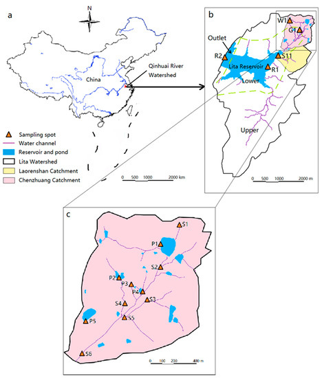
Figure 1.
(a) Geographical location of study area, (b) spatial distribution of sampling sites in Lita Watershed, and (c) the enlarged figure represents the sampling sites in the Chenzhuang Catchment.
The outlet of Lita Watershed, Lita Reservoir (capacity 5.9 million m3), is one of the drinking water sources of Jurong City. Lita Reservoir also provides irrigation supply for surrounding villages scattering in an area of 8.1 km2. Furthermore, Lita Watershed is the Water Conservation Zone of Qinhuai River Watershed (Figure 1a), which flows through Nanjing City, the provincial capital with a population over 8.4 million.
As a mountainous rural watershed of Maoshan Mountain, main land-use types in Lita Watershed are forest, plantation, paddy, construction, and water body. The study area is divided into three regions, the upper, the lower, and the outlet (Figure 1b). In the upper regions, forest occupies the area of around half, and in the lower parts, the percentage of forest, plantation, and paddy are 25%, 28%, and 22%, separately. The area of water bodies is around 12% in whole watershed, and for construction, the percentage is less than 8%. Also, paddies are distributed near the stream to take advantage of the irrigation, and close to ponds, construction and poultry culture are common. Forest and plantation are often located in the sites which are far away from water. In Lita Watershed, the main species in plantation is beeches, which are less than five years, but the beech trees need fertilization.
Inside Lita Watershed, two subcatchments (Laorenshan and Chenzhuang) were chosen for comparison as they had different landscape and human activities. Two subcatchments were chosen for detailed and compared study, the Laorenshan Catchment (Figure 1b) and the Chenzhang Catchment (Figure 1b and enlarged in Figure 1c). Laorenshan Catchment has low development intensity, since less than 15% of lands are plantations and only about 5% are constructions. In contrast, in the Chenzhuang Catchment, the proportions of paddies, plantations, waters, and constructions are 22%, 21%, 13%, and 12%, separately. Meanwhile, the water bodies are various in Chenzhuang Catchment, including streams, ponds, and well waters, while in Laorenshan Catchment, only stream water was studied.
2.2. Water Sampling
Surface water and ground water were sampled in Lita Watershed with the following array: Thus, for water body types, there are pond (P1–P5), stream (S1–S6 and S11), reservoir (R1–R2), wetland (W1), and well (G1). The configurations of these water bodies are presented in Table 1, including the depth, width, and flow for streams, and the area and capacity for ponds, wetland, and reservoir.

Table 1.
Configurations of main water bodies in Lita Watershed.
Taking locations into concern, there are upper (S1–S4), outlet (R2) and the rest are lower ones, as shown in Figure 1b,c. Water samples were collected every month from 2015 to 2016 by sampling bottles. Taking the pollution sources and conditions, 18 water quality indices are measured including discharge (Dis), temperature (TEM), dissolved oxygen (DO), total nitrogen (TN), nitrate nitrogen (NO3), nitrite nitrogen (NO2), ammonia nitrogen (NH4), total phosphorus (TP), phosphate phosphorus (PO4), chemical oxygen demand (COD), arsenic (As), cadmium (Cd), chromium (Cr), copper (Cu), mercury (Hg), manganese (Mn), nickel (Ni), lead (Pb), and Zinc (Zn). The standard methods [51] are introduced in the laboratory work of testing. All the water quality variables, units, analytical methods, and lowest detected limit are displayed in Table 2.
Table 2.
Water quality variables, units, analytical methods, and lowest detected limit of Lita Watershed from 2015 to 2016.
The GIS data, including DEM and land-use types, are derived from Remote Sense Images and other materials. The DEM data are obtained from the ASTER GDEM database with the resolution of 30 m, 2009, and the land-use data are obtained from the LANDSAT 8 database with the resolution of 30 m, 2015. The stream ways and catchment divisions in the study area are firstly generated through ArcSWAT on ArcGIS 10.4.1 basing on the DEM, and then amended manually basing on the remote sensing data from the LANDSAT 8 database with the resolution of 30 m, 2015. Field work has taken place during 2015–2017 to test the real land-use patterns and correct the hydrological catchment division [52]. The meteorological data, including daily average temperature and precipitation, were gained from an automatic observation system located inside the watershed. In addition, the automatic observation tools were also used in recording the flow of outlet section data hourly by Infrared Detectors.
2.3. Statistical Analysis Methods
Spatial and temporal analyses took place in order to figure out the general characteristics of water body types and seasonality. To specify, the spatial analyses include the variation analysis and spatial cluster analysis, and the temporal analyses are mainly based on seasonal analysis. Afterwards, multivariate analyses of the water quality parameters were processed by hierarchical cluster analysis (HCA), Pearson’s Linear Correlation (PLC), principal component analysis (PCA) and Canonical correlation analysis (CCA).
HCA was employed to describe the relationship through groups basing on the similarities within a class and dissimilarities among different classes. In HCA, clusters are formed stepwise by means of the Ward’s method; using squared Euclidean distances cluster significance of 16 sampling sites was determined, the results of which can help explain the data and indicate patterns.
PLC was used and the matrix of correlation efficient was generated. In the system of PCA, firstly, discriminate analysis (DA) was introduced, which is based on discriminant functions (DF) for each group as in Equation (1) [53]):
where i is the number of groups (G); Ki is the constant inherent to each group; n is the number of parameter sets in the certain group; and Wij is the weight coefficient assigned by DF to a given selected parameter Pij.
To standardize, forward stepwise and backward stepwise modes were employed to assess both the spatial and temporal variations of water quality through seasons and water body types. Then, varifactors were generated by principal component through Equation (2) [53]:
where Z is the component score; i is the component number; j is the sample number; A is the component loading; X is the measured value of a variable; and n is the total number of variables. Finally, the most influential factors were found and the component scores were added, the basic concept of which is described in Equation (3) [53]:
where Z is the component score; i is the component number; j is the sample number; A is the component loading; f is the factor score; X is the measured value of a variable; n is the total number of variables; and E is the residual term accounting for errors or other sources of variation.
Canonical correlation analysis (CCA) was also applied in this study as a comparison and a deeper analysis. CCA is a cross-covariance matrix using the correlation between the comprehensive variables to reflect the overall correlation between the two groups of indicators. Its basic principle is: in order to grasp the correlation between the two groups of indicators in general, two representative comprehensive variables, U1 and V1, are extracted from the two groups of variables, which means that the linear combination of each variable in the two groups, respectively, and the correlation between the two comprehensive variables, is used to reflect the overall correlation between the two groups of indicators [54,55,56]. In this study, CCA was introduced to identify the impact power of land-use patterns on water quality parameters. Thus, the land-use patterns were viewed as environment factors, and the sampling sites were viewed as samples.
The usage of software is listed below. ArcGIS 10.4.1 is used for spatial data processing and mapmaking of Figure 1, and the figures, from Figure 2 to Figure 5, were made by R for Windows 3.6.1, Origin 2017 SR2, IBM SPSS Statistics 20 and Canoco for Windows 4.54, namely.
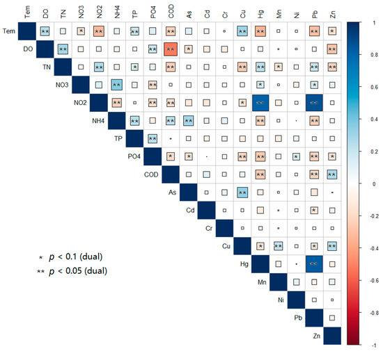
Figure 2.
Matrix of Pearson correlation coefficients among water quality parameters.
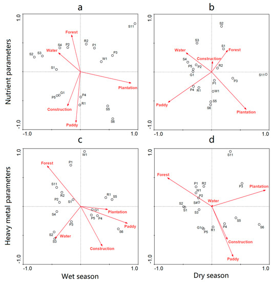
Figure 5.
Canonical correlation analysis (CCA) between seasons and parameter groups basing on land-use patterns (red arrows) and sampling sites (open circles). (a) Nutrient parameters in wet season; (b) Nutrient parameters in day season; (c) Heavy metal parameters in wet season; and (d) heavy metal parameters in dry season.
3. Results
3.1. Spatial and Temporal Variations of Water Quality
The concentration of water quality parameters were tested and are shown in Table 3 and Table 4. The character of temporal variation can be simply described as the values are lower in the wet season for major parameters, but there are exceptions since, for TN, TP, PO4, and NH4, they are higher in the wet season than in the dry season. Interesting, the concentration of Hg and Pb are extremely high in November when compared with other months, and spatially, the outlet and upper regions have a lower index than lower regions. However, TN and COD are higher in the upper region and outlet. While heavy metals usually have alternative character to nutrients, thus, the values of the outlet ones and lower ones are close. The concentrations of Hg and Pb are extremely high in November when compared with other months.
Table 3.
Spatial and temporal variation of aquatic nutrient concentration in Lita Watershed.
Table 4.
Spatial and temporal variation of aquatic heavy metal concentration in Lita Watershed.
3.2. Sensitivity of Water Quality Parameters
Sensitivity of water quality parameters were analyzed through Pearson’s correlation analysis and the principle component analysis Matrix of Pearson correlation coefficients were displayed with the marked significance range (Figure 2). The coefficients with the absolute values larger than 0.6 are significant (p < 0.05), and the values between 0.3 and 0.6 are slightly significant (p < 0.1). Some parameters tend to be more sensitive and have several correlation linkages with other parameters, which are TEM, DO, TN, NO2, NH4, PO4, Cu, Hg, Pb, and Zn, namely, and the rest are insensitive. The most robust correlation pairs exist in both inside and inter groups, the robust correlation pairs exist such as PbHg and HgNO2. Meanwhile, the numbers of positive and negative coefficients are almost the same, but the most robust linear relationships are the positive ones.
Basing on the correlation analysis and the analysis of PCA, the most changeable parameters were found and compared (Figure 3). For the sensitive parameters, Cr, NO3, NO2, and COD, namely, shared the absolute values of over 0.75 in PC1 and PC2 through PCA, while the absolute values of others are less than 0.60. Temporally, the values of all the four parameters are higher in the dry season in the boxplots and the simulated normal distribution curves (Figure 3). The real difference between is diminished due to the using of logarithmic scales. However, the spatial variations are unlikely to be obviously different, which are more scattering distributed. Additionally, COD and NO2 are widely distributed in certain sites, and Cr and NO3 are narrowed, and phenomenon is similar through seasons.
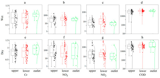
Figure 3.
Distributions of the most significant parameters during wet and dry seasons. The bars indicate the upper and lower quarter of distributions; the horizontal lines, from upper to lower, indicate the extreme large values, median values, and small values; and the points inside the bars represent the mean values. (a) Cr in wet season; (b) NO3 in wet season; (c) NO2 in wet season; (d) COD in wet season; (e) Cr in dry season; (f) NO3 in dry season; (g) NO2 in dry season; and (h) COD in dry season.
3.3. Spatial Similarity of Sampling Sites
Effect of landscapes on water quality can be studied in several aspects, including the location and types of water bodies, and land-use patterns. Therefore, hierarchical clustering method was used to assess the similarity of sampling sites, and the dendograms were yielded and displayed in Figure 4. In Figure 4, the clusters indicate the similarity of sampling sites, and the distances are computed by Ward’s method, using squared Euclidean distances processes, and the scales illustrate the differences of the coherence among sampling sites.
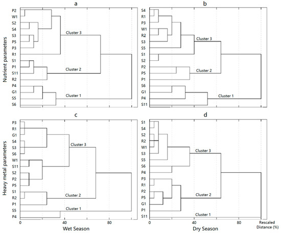
Figure 4.
Spatial hierarchical cluster of sampling sites in Lita Watershed. (a) Nutrient parameters in wet season; (b) Nutrient parameters in dry season; (c) Heavy metal parameters in wet season; and (d) heavy metal parameters in dry season.
It is clear that distributions of nutrient parameters are more various than heavy metals. The reason lies in that there are clusters of only one or two members (Cluster 1 in Figure 4c,d) in the graphs of heavy metal parameters, but this phenomenon disappears in the graphs of nutrient parameters (Figure 4a,b). Also inside the clusters of nutrients, the elements are close to each other, but for heavy metal, the distances are usually far. Temporally, nutrients are steadier between wet and dry seasons than heavy metals, which means that the latter ones are more sensitive to seasonal changes.
3.4. Influence of Land-Use Patterns on Water Quality
Canonical correlation analysis (CCA) was introduced here to detect the interaction between land-use types and sampling sites and the biplots are presented in Figure 5. The red arrows represent the land-use patterns and the open circles represent sampling sites. The intersection angles between arrows indicate the relationships. To clarify, the acute angle represents positive correlation, and the smaller angle represents the greater positive correlation coefficient; the obtuse angle represents negative correlation, and the larger angle represents the greater absolute value of negative correlation coefficient; the right angle represents uncorrelation, and the angle close to right angle represents the weak correlation. Also, for points, the distance between the point and the arrow line means the relationship between them; thus, a short distance for a strong relationship. Generally, the graph patterns are more similar from seasons than from parameter groups. In detail, the patterns of nutrients, heavy metals, and sampling sites are illustrated separately. For nutrients, the plantation has different characters from other land-use sorts (Figure 5a,b), and the arrow of water body is close to the opposite direction of plantation. For heavy metal, forest is the opposite one to others, which is obviously different to the distributions of arrows (Figure 5a,b). The distribution of points means the similarity among sampling sites. In the wet season, the points are more scattered, and in the dry season, they are concentrated (Figure 5a,b). This pattern is the same for both nutrients and heavy metals.
4. Discussion
4.1. Source Identification of Aquatic Heavy Metals and Nutrients
The spatial distribution of heavy metals in Lita Watershed showed the mix patterns through wet and dry seasons (Table 4 and Figure 2). For instance, the temporal distribution patterns of heavy metal have the opposite characters to the nitrogen and phosphorus. Also, the seasonal difference is significant, as the peak of pollution often occurred in November and December in 2015 and 2016, while during this period of dry season, the concentration of nutrients remained in the low level. Furthermore, an interesting finding is that, in Figure 4a,c, the upper site S2 and the lower site P5 share the same cluster with short distance. However, the upper regions less affected by anthropogenic aspects are unlikely to have the similar characters of the lower regions. So, there should be some sources of pollutants with slight linkages with locations.
In order to compare the results and identify the sources of heavy metals, the results of similar studies were presented in Table 5.
Table 5.
Concentration of heavy metals from this study and comparable researches.
The aquatic heavy metal is mainly caused by point pollution, such as energy production, manufacturing, and transport [64,65,66]. Other than the industrial area, there were no obvious industrial activities in Lita Watershed during 2015 and 2016. Some studies demonstrated that the fertilization, fecal discharge, and the incineration and burial of waste can also be the drivers of heavy metal, the process of pollution can be conveyed through soil, not directly [58,67]. However, the amount of these tracing elements by nonpoint sources is at the low level [68] (pp. 657–678), [69]; for instance, the concentration of Hg and Pb in water are unlikely to surpass 2.0 μg·L−1 in surface water samples when the amount of water is ample [57,59]. Therefore, nonpoint source is unlikely to be the main source of heavy metal.
As a result, the wet and dry depositions are the major source of heavy metal in this study, especially for Hg and Pb. Our study area is located in an industrialized region, Yangtze River Delta and surrounded by several large cities, including Shanghai, Suzhou, and Nanjing [67,70]. Moreover, during autumn and winter, the strong monsoon can carry the pollution from Northern China, and several recent studies indicated the linkage between industry and heavy metal pollution in water [50,60]. By consulting similar areas, the concentrations of Hg and Pb are close to those in Lita Watershed [61].
The source identifying and moving mechanism of nutrients among water bodies and land-use patterns can also be introduced to explain the parameters of heavy metals according to the correlation coefficient matrix (Figure 2). The pairs of most significant linear relationships can be grouped by three clues, the inherent properties, seasonality, and sources. For inherent properties, the negative relationship between DO and COD is obvious. For seasonality, in the wet season, the temperature is high, and the concentration of TN and TP is usually relatively high, while in the dry season, the concentration of NO2 is high in this study, as well as some heavy metals, including Hg and Pb. Thus, the negative correlation pairs (Tem-Hg, Tem-Pb, and Tem-NO2) and positive correlation pairs (Hg-NO2 and Pb-NO2) can be explained [46,50]. For sources, the NO3 and NH4 are different forms of nitrogen element, and can be transformed to each other. In the countryside of China, both fertilization and fecal discharge are contributed to NO3 and NH4, and this phenomenon is also being studied in recent researches [8,9,46]. Another pair with similar sources is Pb and Hg, mainly in power plants [71,72], so the positive correlation is apparent.
4.2. Water Body Configurations, Land-Use Patterns and Their Driving Effects on Water Quality
In this study area, Lita Watershed, and many other similar watersheds in the Southern China, the type of water bodies is various, as well as their effects on water quality. For example, differing to lakes and reservoirs, pond water is well mixed, and less protected, and the quality of water is strongly determined by the environment and condition in vicinity, not the whole watershed. Generally, the water quality is degraded gradually from S1 to S6 and from P1 to P5, but for reservoirs, the outlet water is much better than the inlet one, which indicates the effect of purifying, and the clue is revealed by the fact that the outlet is included in the same cluster with the upper sites. Other than locations, this article attempts to trace the linkage between the configurations of water bodies (Table 1) and their influence on water quality.
The scale of water bodies is an important factor to influence water quality. For ponds in the similar region, the larger ones tend to have cleaner water, taking P1 and P2 for instance. However, this phenomenon is not obvious in stream water. The reason can be that the amount of stream water is changeable during seasons, so the downstream water can be less than the upper one in several times. Two special water bodies, the wetland water and ground water, are extremely different; thus, the former is one of the best and the latter is the worse. The plants in wetland can clean up water [73], and the paddies have the similar function. In this study, the site W1 is the upper region perennial wild wetland, so the water quality can be higher. When taking groups of water quality variables into concern, pond water, reservoir water, and ground water are more likely to be affected by heavy metal pollutions than river water. The solution can be found in two aspects, the interaction between air and the soil, pond water, and reservoir water tend to be dominated by the first factor, and the second factor for ground water [74,75,76].
The land-use types and the activities on the certain types (fertilization, irrigation, aquaculture, and heaviest) have the indirect influence on water quality [41,77,78]. The plantation is opposite to the others due to the large amount of fertilizer and less water (Figure 5a,b); as in the study area, the amounts of fertilizer in plantations are large [9]. Paddies are also heavily fertilized, but the effect of water dilution and the quick absorption of rice plant decreases the accumulation of nutrients greatly [27,79]. Also, Figure 5a,b imply that the arrow of water body is close to the opposite direction of plantation, which means that the dilution effect of water body is important, and for sampling sites, the ones with the best water quality are located in the first quadrant. Additionally, after our study period, thus, during 2017 and 2018, there were extreme land-use changes within Chenzhuang Watershed. As a result, influence of certain land-use patterns on water quality needs an alternative focus on the land-use changes.
Several researches demonstrated that the forest can reduce the air deposition of heavy metals [80,81], which is similar to this study, as the forest has the opposite effect to the others (Figure 5c,d). Then for plantation, the leaf area index (LAI) is low, which means that the beech trees are too small to absorb enough heavy metal, and the differences of the ecological functions between plantation and forests are concerned by other studies [27,82]. Additionally, the scattered distribution of points in Figure 5c,d may be evidence to support that the source of heavy metals is mainly from air, not water [83].
4.3. Management Implications
Water quality in headwater area is fundamental for drinking water and food safety. In densely populated and rapid industrialized areas of China, systematic assessment and management of headwater catchment is urgent. According to the results and analysis of this study, policy of headwater protection can be attributed into three steps. First, reservoir plays the key role in water conservation, and the purifying effect is significant (Figure 4). Therefore, the activities upon the reservoir should be forbidden, including poultry culturing and tourist industry. Also, maintaining the water level and capability of the reservoir can help fulfill its function [16].
Second, upstream protection is the effective way to reduce the pollutant discharging. Many studies demonstrated that the construction of forest-soil buffer zones and other engineering actions taken on soils can bring benefits to reducing pollution [27,84]. However, this study points out that making good use of water body systems is also important (Table 3 and Table 4). For illustration, the pond systems are used for interception, reservation, and sediment, and the streams systems are used for water supply. In Southeastern China, the paddies and other seasonal water bodies have similar functions as the ponds. Two main factors decide the functions of water bodies, the scales, and the land-use patterns in the subcatchment. So, taking the scales of paddies into concern, in the wet season, the paddies dominate the function of water purifying while, in the dry season, ponds take the role. For land-use patterns, forest, grass, and paddies, having good water capacities themselves, are less reliant on the water bodies for pollution reducing, but construction is opposite. The large subcatchments with big amounts of pollutant need to match the water bodies with high proportions and various types (Figure 1 and Figure 4). Other researches also demonstrated that the upper regions with forest mainly usually can cut off 30% of nitrogen and phosphorus leaking than the lower regions with croplands and urban areas mainly [9,27,78]. Experiences in Lita Watershed can be applied in two situations, the areas where the water body types and shapes are adjustable and where the soil management is hard to realize.
Third, tracing the temporal and spatial variation of water quality parameters can help in finding the shortcut to improve water quality. The management can be described from two aspects. Clues between seasonal distribution of nutrients and heavy metals reveal their sources and movements. Moreover, the relationships among different parameters also contribute to the targeted solutions based on pollution reduction. Also, studies and practices provide evidence that the optimal watershed plan can reduce the risk of flood and other disasters, and benefit the economy and society [85,86].
5. Conclusions
Basing on the multistatistics analysis on Lita Reservoir, landscapes have strong influence on headwater quality in both groups of nutrient parameters and heavy metal parameters. Results show that the most sensitive water quality parameters are Cr, NO3, NO2, and COD. The configurations of water bodies (location, types, and scales) are the direct factors to determine the effect of reducing the water pollution, while land-use patterns in the surrounding area have the indirect effect on the movement of pollutants. The influence of landscape on water quality is more sensitive in the aspect of season rather than parameters. This finding means that adjusting the water body configurations and land-use patterns can reduce the loads of contaminants from fertilization and poultry farming significantly, but remain to be useless for heavy metals. These findings and regulations are useful for making the targeted plans on headwater protections in three aspects: source identifying and controlling, water body tracing and adjusting, and predicting and early warning of water pollution events. Additional studies and practical water quality models in monsoon controlled small watersheds are needed to quantify the relationship among water quality parameters in order to make refinement managements.
Author Contributions
Funding acquisition, W.D. and W.C. (Wenjun Chen); investigation, W.C. (Wen Chen), H.Z., and B.H.; project administration, H.W., W.S., H.Z., and B.H.; writing—original draft, K.Z.; writing—review & editing, H.W., W.S., and B.H. All authors have read and agreed to the published version of the manuscript.
Funding
This research was funded by “One-Three-Five” Strategic Planning of Nanjing Institute of Geography and Limnology, Chinese Academy of Sciences, grant number NIGLAS2017GH06 and NIGLAS2017GH07; the Strategic Priority Research Program of the Chinese Academy of Sciences, grant number XDA23020102; the GDAS’ Project of Constructing Domestic First Class Institution, grant number 2020GDASYL-20200102013, 2020GDASYL-20200301003 and 2019GDASYL-0102002 and the National Natural Science Foundation of China, grant number 41871119.
Acknowledgments
We would like to thank Meng Huifang, Yang Chaojie, Wu Yanjuan, and Liu Xiangnan for their field work.
Conflicts of Interest
The authors declare no conflict of interest.
References
- Ahuja, S.S.; Larsen, M.C.; Eimers, J.L. Comprehensive Water Quality and Purification, Chapter: Volume 1: Status and Trends of Water Quality Worldwide; Elsevier: Calabash, NC, USA, 2014. [Google Scholar]
- Ferrier, R.C.; Edwards, A.C.; Hirst, D.; Littlewood, I.G.; Watts, C.D.; Morris, R. Water quality of Scottish rivers: Spatial and temporal trends. Sci. Total. Environ. 2001, 265, 327–342. [Google Scholar] [CrossRef]
- Panagoulia, D. Impacts of GISS-modelled climate changes on catchment hydrology. Hydrol. Sci. J. 1992, 37, 141–163. [Google Scholar] [CrossRef]
- Panagoulia, D.; Dimou, G. Sensitivities of groundwater-streamflow interaction to global climate change. Hydrol. Sci. J. 1996, 41, 781–796. [Google Scholar] [CrossRef]
- Vörösmarty, C.J.; Green, P.; Salisbury, J.; Lammers, R.B. Global Water Resources: Vulnerability from Climate Change and Population Growth. Science 2000, 289, 284–288. [Google Scholar] [CrossRef]
- Han, D.; Currell, M.J.; Cao, G. Deep challenges for China’s war on water pollution. Environ. Pollut. 2016, 218, 1222–1233. [Google Scholar] [CrossRef]
- Wang, Q.; Yang, Z. Industrial water pollution, water environment treatment, and health risks in China. Environ. Pollut. 2016, 218, 358–365. [Google Scholar] [CrossRef]
- Carpenter, S.R.; Caraco, N.F.; Correll, D.L.; Howarth, R.W.; Sharpley, A.N.; Smith, V.H. Nonpoint Pollution of Surface Waters with Phosphorus and Nitrogen. Ecol. Appl. 1998, 8, 559–568. [Google Scholar] [CrossRef]
- Chen, W.; He, B.; Nover, D.; Duan, W.; Luo, C.; Zhao, K.; Chen, W. Spatiotemporal patterns and source attribution of nitrogen pollution in a typical headwater agricultural watershed in Southeastern China. Environ. Sci. Pollut. Res. 2018, 25, 2756–2773. [Google Scholar] [CrossRef]
- European Environmental Agency. Appendix A: Definitions of Water Resources. 2016. Available online: https://www.eea.europa.eu/publications/92-9167-056-1/page017.html (accessed on 14 January 2020).
- Khan, S.; Shahnaz, M.; Jehan, N.; Rehman, S.; Shah, M.T.; Din, I. Drinking water quality and human health risk in Charsadda district, Pakistan. J. Clean. Prod. 2013, 60, 93–101. [Google Scholar] [CrossRef]
- Wu, C.; Maurer, C.; Wang, Y.; Xue, S.; Davis, D.L. Water pollution and human health in China. Environ. Heal. Perspect. 1999, 107, 251–256. [Google Scholar] [CrossRef]
- Bartram, J.; Cotruvo, J.; Exner, M.; Fricker, C.; Glasmacher, A. Heterotrophic Plate Counts and Drinking-Water Safety: The Significance of HPCs for Water Quality and Human Health; World Health Organization: Denver, CO, USA, 2003; Volume 12. [Google Scholar] [CrossRef]
- Dechesne, M.; Soyeux, E. Assessment of Source Water Pathogen Contamination. J. Water Heal. 2007, 5, 39–50. [Google Scholar] [CrossRef]
- Müller, B.; Berg, M.; Yao, Z.P.; Zhang, X.F.; Wang, D.; Pfluger, A. How polluted is the Yangtze river? Water quality downstream from the Three Gorges Dam. Sci. Total. Environ. 2008, 402, 232–247. [Google Scholar] [CrossRef] [PubMed]
- Wei, G.; Yang, Z.; Cui, B.; Li, B.; Chen, H.; Bai, J.; Dong, S. Impact of Dam Construction on Water Quality and Water Self-Purification Capacity of the Lancang River, China. Water Resour. Manag. 2009, 23, 1763–1780. [Google Scholar] [CrossRef]
- Delpla, I.; Jung, A.-V.; Baures, E.; Clement, M.; Thomas, O. Impacts of climate change on surface water quality in relation to drinking water production. Environ. Int. 2009, 35, 1225–1233. [Google Scholar] [CrossRef] [PubMed]
- Immerzeel, W.W.; van Beek, L.P.H.; Bierkens, M.F.P. Climate Change Will Affect the Asian Water Towers. Science 2010, 328, 1382–1385. [Google Scholar] [CrossRef]
- McMillan, H.; Krueger, T.; Freer, J. Benchmarking observational uncertainties for hydrology: Rainfall, River discharge and water quality. Hydrol. Process. 2012, 26, 4078–4111. [Google Scholar] [CrossRef]
- Yaziz, M.I.; Gunting, H.; Sapari, N.; Ghazali, A.W. Variations in rainwater quality from roof catchments. Water Res. 1989, 23, 761–765. [Google Scholar] [CrossRef]
- Issaka, S.; Ashraf, M.A. Impact of soil erosion and degradation on water quality: A review. Geol. Ecol. Landscapes 2017, 1, 1–11. [Google Scholar] [CrossRef]
- Pimentel, D.; Harvey, C.; Resosudarmo, P.; Sinclair, K.; Kurz, D.; McNair, M.; Crist, S.; Shpritz, L.; Fitton, L.; Saffouri, R.; et al. Environmental and Economic Costs of Soil Erosion and Conservation Benefits. Science 1995, 267, 1117. [Google Scholar] [CrossRef]
- Zarris, D.; Vlastara, M.; Panagoulia, D. Sediment delivery assessment for a transboundary Mediterranean catchment: The example of Nestos River Catchment. Water Resour. Manag. 2011, 25, 3785–3803. [Google Scholar] [CrossRef]
- Chang, M.; McBroom, M.W.; Scott Beasley, R. Roofing as a source of nonpoint water pollution. J. Environ. Manag. 2004, 73, 307–315. [Google Scholar] [CrossRef] [PubMed]
- Jabbar, F.K.; Grote, K. Statistical assessment of nonpoint source pollution in agricultural watersheds in the Lower Grand River watershed, MO, USA. Environ. Sci. Pollut. Res. 2019, 26, 1487–1506. [Google Scholar] [CrossRef] [PubMed]
- Polyakov, V.; Fares, A.; Ryder, M.H. Precision riparian buffers for the control of nonpoint source pollutant loading into surface water: A review. Environ. Rev. 2005, 13, 129–144. [Google Scholar] [CrossRef]
- Ding, J.; Jiang, Y.; Liu, Q.; Hou, Z.; Liao, J.; Fu, L.; Peng, Q. Influences of the land use pattern on water quality in low-order streams of the Dongjiang River basin, China: A multi-scale analysis. Sci. Total. Environ. 2016, 551, 205–216. [Google Scholar] [CrossRef] [PubMed]
- Lee, S.-W.; Hwang, S.-J.; Lee, S.-B.; Hwang, H.-S.; Sung, H.-C. Landscape ecological approach to the relationships of land use patterns in watersheds to water quality characteristics. Landsc. Urban. Plan. 2009, 92, 80–89. [Google Scholar] [CrossRef]
- Lewis, W.M., Jr.; Saunders, J.F., III. Concentration and Transport of Dissolved and Suspended Substances in the Orinoco River. Biogeochemistry 1989, 7, 203–240. [Google Scholar] [CrossRef]
- Alberti, M.M.; Booth, D.D.; Hill, K.K.; Coburn, B.B.; Avolio, C.C.; Coe, S.; Spirandelli, D. The impact of urban patterns on aquatic ecosystems: An empirical analysis in Puget lowland sub-basins. Landsc. Urban Plan. 2007, 80, 345–361. [Google Scholar] [CrossRef]
- Donohue, I.; McGarrigle, M.L.; Mills, P. Linking catchment characteristics and water chemistry with the ecological status of Irish rivers. Water Res. 2006, 40, 91–98. [Google Scholar] [CrossRef]
- Johnson, L.; Richards, C.; Host, G.; Arthur, J. Landscape influences on water chemistry in Midwestern stream ecosystems. Freshw. Boil. 1997, 37, 193–208. [Google Scholar] [CrossRef]
- Ding, J.; Jiang, Y.; Fu, L.; Liu, Q.; Peng, Q.; Kang, M. Impacts of Land Use on Surface Water Quality in a Subtropical River Basin: A Case Study of the Dongjiang River Basin, Southeastern China. Water 2015, 7, 4427–4445. [Google Scholar] [CrossRef]
- Bu, H.; Meng, W.; Zhang, Y.; Wan, J. Relationships between land use patterns and water quality in the Taizi River basin, China. Ecol. Indic. 2014, 41, 187–197. [Google Scholar] [CrossRef]
- Gémesi, Z.; Downing, J.A.; Cruse, R.M.; Anderson, P.F. Effects of Watershed Configuration and Composition on Downstream Lake Water Quality. J. Environ. Qual. 2011, 40, 517–527. [Google Scholar] [CrossRef] [PubMed]
- Dodds, W.K.; Oakes, R.M. Headwater Influences on Downstream Water Quality. Environ. Manag. 2008, 41, 367–377. [Google Scholar] [CrossRef] [PubMed]
- Sun, R.; Chen, L.; Chen, W.; Ji, Y. Effect of Land-Use Patterns on Total Nitrogen Concentration in the Upstream Regions of the Haihe River Basin, China. Environ. Manag. 2013, 51, 45–58. [Google Scholar] [CrossRef]
- Solanki, V.R.; Hussain, M.M.; Raja, S.S. Water quality assessment of Lake Pandu Bodhan, Andhra Pradesh State, India. Environ. Monit. Assess. 2010, 163, 411–419. [Google Scholar] [CrossRef] [PubMed]
- Lu, Y.; Song, S.; Wang, R.; Liu, Z.; Meng, J.; Sweetman, A.J.; Jenkins, A.; Ferrier, R.C.; Li, H.; Luo, W.; et al. Impacts of soil and water pollution on food safety and health risks in China. Environ. Int. 2015, 77, 5–15. [Google Scholar] [CrossRef]
- Reza, R.; Singh, G. Heavy metal contamination and its indexing approach for river water. Int. J. Environ. Sci. Technol. 2010, 7, 785–792. [Google Scholar] [CrossRef]
- Arora, M.; Kiran, B.; Rani, S.; Rani, A.; Kaur, B.; Mittal, N. Heavy metal accumulation in vegetables irrigated with water from different sources. Food Chem. 2008, 111, 811–815. [Google Scholar] [CrossRef]
- Singh, A.; Sharma, R.K.; Agrawal, M.; Marshall, F.M. Health risk assessment of heavy metals via dietary intake of foodstuffs from the wastewater irrigated site of a dry tropical area of India. Food Chem. Toxicol. 2010, 48, 611–619. [Google Scholar] [CrossRef]
- Almeida, C.A.A.; Quintar, S.; Gonzalez, P.; Mallea, M.A. Influence of Urbanization and Tourist Activities on the Water Quality of the Potrero de Los Funes River (San Luis-Argentina). Environ. Monit. Assess. 2007, 133, 459–465. [Google Scholar] [CrossRef]
- Sanchez, E.; Colmenarejo, M.F.; Vicente, J.; Rubio, A.; García, M.G.; Travieso, L.; Borja, R. Use of the Water Quality Index and Dissolved Oxygen Deficit as Simple Indicators of Watersheds Pollution. Ecol. Indic. 2007, 7, 315–328. [Google Scholar] [CrossRef]
- Lumb, A.; Halliwell, D.; Sharma, T. Application of CCME Water Quality Index to Monitor Water Quality: A Case Study of the Mackenzie River Basin, Canada. Environ. Monit. Assess. 2006, 113, 411–429. [Google Scholar] [CrossRef] [PubMed]
- Wu, Z.; Wang, X.; Chen, Y.; Cai, Y.; Deng, J. Assessing river water quality using water quality index in Lake Taihu Basin, China. Sci. Total. Environ. 2018, 612, 914–922. [Google Scholar] [CrossRef]
- Leung, A.O.W.; Duzgoren-Aydin, N.S.; Cheung, K.C.; Wong, M.H. Heavy Metals Concentrations of Surface Dust from e-Waste Recycling and Its Human Health Implications in Southeast China. Environ. Sci. Technol. 2008, 42, 2674–2680. [Google Scholar] [CrossRef] [PubMed]
- Xing, Y.; Lu, Y.; Dawson, R.W.; Shi, Y.; Zhang, H.; Wang, T.; Liu, W.; Ren, H. A spatial temporal assessment of pollution from PCBs in China. Chemosphere 2005, 60, 731–739. [Google Scholar] [CrossRef] [PubMed]
- Zhang, Z.L.; Hong, H.S.; Zhou, J.L.; Huang, J.; Yu, G. Fate and assessment of persistent organic pollutants in water and sediment from Minjiang River Estuary, Southeast China. Chemosphere 2003, 52, 1423–1430. [Google Scholar] [CrossRef]
- Duan, W.; He, B.; Nover, D.; Yang, G.; Chen, W.; Meng, H.; Zou, S.; Liu, C. Water Quality Assessment and Pollution Source Identification of the Eastern Poyang Lake Basin Using Multivariate Statistical Methods. Sustainability 2016, 8, 133. [Google Scholar] [CrossRef]
- GB5749-2006. P. R. China Standards for Drinking Water Quality; Department of Health, P.R. China: Beijing, China, 2006. [Google Scholar]
- Karikari, A.Y.; Ansa-Asare, O.D. Physico-Chemical and Microbial Water Quality Assessment of Densu River of Ghana. West. Afr. J. Appl. Ecol. 2009, 10. [Google Scholar] [CrossRef]
- Khattree, R.; Naik, D.N. Applied Multivariate Statistics with SAS Software, 2nd ed.; SAS Institute Inc.: Cary, NC, USA, 2018. [Google Scholar]
- Hejcmanovā-Nežerková, P.; Hejcman, M. A canonical correspondence analysis (CCA) of the vegetation–environment relationships in Sudanese savannah, Senegal. South. Afr. J. Bot. 2006, 72, 256–262. [Google Scholar] [CrossRef]
- Khalil, B.; Ouarda, T.B.M.J.; St-Hilaire, A. Estimation of water quality characteristics at ungauged sites using artificial neural networks and canonical correlation analysis. J. Hydrol. 2011, 405, 277–287. [Google Scholar] [CrossRef]
- Noori, R.; Sabahi, M.S.; Karbassi, A.R.; Baghvand, A.; Taati Zadeh, H. Multivariate statistical analysis of surface water quality based on correlations and variations in the data set. Desalination 2010, 260, 129–136. [Google Scholar] [CrossRef]
- Qu, B.; Zhang, Y.; Kang, S.; Sillanpää, M. Water quality in the Tibetan Plateau: Major ions and trace elements in rivers of the “Water Tower of Asia”. Sci. Total. Environ. 2019, 649, 571–581. [Google Scholar] [CrossRef] [PubMed]
- Yin, S.; Feng, C.; Li, Y.; Yin, L.; Shen, Z. Heavy metal pollution in the surface water of the Yangtze Estuary: A 5-year follow-up study. Chemosphere 2015, 138, 718–725. [Google Scholar] [CrossRef] [PubMed]
- Yang, Z.; Wang, Y.; Shen, Z.; Niu, J.; Tang, Z. Distribution and speciation of heavy metals in sediments from the mainstream, tributaries, and lakes of the Yangtze River catchment of Wuhan, China. J. Hazard. Mater. 2009, 166, 1186–1194. [Google Scholar] [CrossRef]
- Wan, D.; Han, Z.; Yang, J.; Yang, G.; Liu, X. Heavy Metal Pollution in Settled Dust Associated with Different Urban Functional Areas in a Heavily Air-Polluted City in North China. Int. J. Environ. Res. Public Heal. 2016, 13, 1119. [Google Scholar] [CrossRef]
- Huang, S.S.; Liao, Q.L.; Hua, M.; Wu, X.M.; Bi, K.S.; Yan, C.Y.; Chen, B.; Zhang, X.Y. Survey of heavy metal pollution and assessment of agricultural soil in Yangzhong district, Jiangsu Province, China. Chemosphere 2007, 67, 2148–2155. [Google Scholar] [CrossRef]
- Rajkumar, H.; Naik, P.K.; Rishi, M.S. Evaluation of heavy metal contamination in soil using geochemical indexing approaches and chemometric techniques. Int. J. Environ. Sci. Technol. 2018, 16, 7467–7486. [Google Scholar] [CrossRef]
- Gaillardet, J.; Dupré, B.; Louvat, P.; Allègre, C.J. Global silicate weathering and CO2 consumption rates deduced from the chemistry of large rivers. Chem. Geol. 1999, 159, 3–30. [Google Scholar] [CrossRef]
- Ali, H.H.; Khan, E.; Sajad, M.A. Phytoremediation of heavy metals—Concepts and applications. Chemosphere 2013, 91, 869–881. [Google Scholar] [CrossRef]
- Bhutiani, R.; Kulkarni, D.B.; Khanna, D.R.; Gautam, A. Water Quality, Pollution Source Apportionment and Health Risk Assessment of Heavy Metals in Groundwater of an Industrial Area in North India. Expo. Health 2016, 8, 3–18. [Google Scholar] [CrossRef]
- Toppi, L.S.; Gabbrielli, R. Response to cadmium in higher plants. Environ. Exp. Bot. 1999, 41, 105–130. [Google Scholar] [CrossRef]
- Chen, H.; Teng, Y.; Lu, S.; Wang, Y.; Wang, J. Contamination features and health risk of soil heavy metals in China. Sci. Total. Environ. 2015, 512, 143–153. [Google Scholar] [CrossRef] [PubMed]
- Feng, X. Dynamics of Mercury Pollution on Regional and Global Scales: Atmospheric Processes and Human Exposures Around the World; Pirrone, N., Mahaffey, K.R., Eds.; Springer: Boston, MA, USA, 2005; pp. 657–678. [Google Scholar]
- Spiegel, S.J. New mercury pollution threats: A global health caution. Lancet 2017, 390, 226–227. [Google Scholar] [CrossRef]
- Yin, S.; Wu, Y.; Xu, W.; Li, Y.; Shen, Z.; Feng, C. Contribution of the upper river, the estuarine region, and the adjacent sea to the heavy metal pollution in the Yangtze Estuary. Chemosphere 2016, 155, 564–572. [Google Scholar] [CrossRef]
- Feng, X.; Qiu, G. Mercury pollution in Guizhou, Southwestern China—An overview. Sci. Total. Environ. 2008, 400, 227–237. [Google Scholar] [CrossRef]
- Li, P.; Feng, X.B.; Qiu, G.L.; Shang, L.H.; Li, Z.G. Mercury pollution in Asia: A review of the contaminated sites. J. Hazard. Mater. 2009, 168, 591–601. [Google Scholar] [CrossRef]
- Liu, Y.; Bralts, V.F.; Engel, B.A. Evaluating the effectiveness of management practices on hydrology and water quality at watershed scale with a rainfall-runoff model. Sci. Total. Environ. 2015, 511, 298–308. [Google Scholar] [CrossRef]
- Boyle, J.F.; Birks, H.J.B. Predicting Heavy Metal Concentrations in the Surface Sediments of Norwegian Headwater Lakes from Atmospheric Deposition: An Application of a Simple Sediment-Water Partitioning Model. Water Air Soil Pollut. 1999, 114, 27–51. [Google Scholar] [CrossRef]
- Ismail, A.; Toriman, M.E.; Juahir, H.; Zain, S.M.; Habir, N.L.A.; Retnam, A.; Kamaruddin, M.K.A.; Umar, R.; Azid, A. Spatial assessment and source identification of heavy metals pollution in surface water using several chemometric techniques. Mar. Pollut. Bull. 2016, 106, 292–300. [Google Scholar] [CrossRef]
- Ukonmaanaho, L.; Starr, M.; Mannio, J.; Ruoho-Airola, T. Heavy metal budgets for two headwater forested catchments in background areas of Finland. Environ. Pollut. 2001, 114, 63–75. [Google Scholar] [CrossRef]
- Zeinalzadeh, K.; Rezaei, E. Determining spatial and temporal changes of surface water quality using principal component analysis. J. Hydrol. Reg. Stud. 2017, 13, 1–10. [Google Scholar] [CrossRef]
- Stefanidis, K.; Papaioannou, G.; Markogianni, V.; Dimitriou, E. Water Quality and Hydromorphological Variability in Greek Rivers: A Nationwide Assessment with Implications for Management. Water 2019, 11, 1680. [Google Scholar] [CrossRef]
- Bordalo, A.A.; Nilsumranchit, W.; Chalermwat, K. Water quality and uses of the Bangpakong River (Eastern Thailand). Water Res. 2001, 35, 3635–3642. [Google Scholar] [CrossRef]
- Hernández, L.; Probst, A.; Probst, J.L.; Ulrich, E. Heavy metal distribution in some French forest soils: Evidence for atmospheric contamination. Sci. Total. Environ. 2003, 312, 195–219. [Google Scholar] [CrossRef]
- Pouyat, R.V.; McDonnell, M.J. Heavy metal accumulations in forest soils along an urban- rural gradient in Southeastern New York, USA. Water Air Soil Pollut. 1991, 57, 797–807. [Google Scholar] [CrossRef]
- Shrestha, S.; Kazama, F. Assessment of surface water quality using multivariate statistical techniques: A case study of the Fuji river basin, Japan. Environ. Model. Softw. 2007, 22, 464–475. [Google Scholar] [CrossRef]
- Wongsasuluk, P.; Chotpantarat, S.; Siriwong, W.; Robson, M. Heavy metal contamination and human health risk assessment in drinking water from shallow groundwater wells in an agricultural area in Ubon Ratchathani province, Thailand. Environ. Geochem. Health 2014, 36, 169–182. [Google Scholar] [CrossRef]
- Altenburger, R.; Ait-Aissa, S.; Antczak, P.; Backhaus, T.; Barceló, D.; Seiler, T.-B.; Brion, F.; Busch, W.; Chipman, K.; de Alda, M.L.; et al. Future water quality monitoring—Adapting tools to deal with mixtures of pollutants in water resource management. Sci. Total Environ. 2015, 512–513, 540–551. [Google Scholar] [CrossRef]
- Tong, S.T.Y.; Chen, W. Modeling the relationship between land use and surface water quality. J. Environ. Manag. 2002, 66, 377–393. [Google Scholar] [CrossRef]
- Wheater, H.; Evans, E. Land use, water management and future flood risk. Land Use Policy 2009, 26, S251–S264. [Google Scholar] [CrossRef]
© 2020 by the authors. Licensee MDPI, Basel, Switzerland. This article is an open access article distributed under the terms and conditions of the Creative Commons Attribution (CC BY) license (http://creativecommons.org/licenses/by/4.0/).