Abstract
In this paper, we investigate price and order strategies for innovative green products using demand forecasting and sharing. We formulate the problem using a Stackelberg game and propose a dynamic contract that specifies an initial wholesale price, a minimum order quantity, a demand sharing agreement, and a decisions adjustment agreement. We arrived at the following main findings and implications. First, the manufacturer offers a higher or lower wholesale price than the initial one depending on the variation in the market status. Also, the retailer’s ordering decisions will increase with the wholesale price, which contradicts the common assumption that ordering decisions decrease with the wholesale price. Interestingly, if the market improves, the manufacturer obtains a higher profit margin than the retailer; if the market worsens, the manufacturer suffers more loss of profit margin than the retailer. Second, when the cost of information sharing is smaller than an upper bound, demand forecasting and sharing are always beneficial to the manufacturer. However, the value of demand forecasting and sharing for the retailer is significantly affected by the market status variation. Third, high information accuracy will not necessarily increase the profits of the manufacturer and the retailer, even if the market status is better than expected. Finally, numerical examples show the parameters’ effects. We have several main managerial insights. When the shared demand information is received from the retailer, the manufacturer can determine wholesale price strategies according to the retailer’s demand forecast. Moreover, if the manufacturer wants to ensure profitability, they should not choose retailers with a higher capability of demand forecasting.
1. Introduction
Sustainable supply chain management (SSCM) has received a lot of attention in recent years [1,2]. SSCM is defined as the management of material, information, and capital flows, as well as cooperation among companies along the supply chain; it takes into account the goals of all three dimensions of sustainable development, i.e., economic, environmental, and social, which are derived from customer and stakeholder requirements [3]. Fashion companies, such as Nike, Marks and Spencer, H&M, and Uniqlo, have all established environmental sustainability programs [4]. Procter & Gamble (P & G) sells eco-friendly skincare products, razor blades, and laundry detergent that use natural and environmentally sensitive raw materials [5,6]. An outdoor product company, North Face, launched a sustainability program in 2011, and established an innovation center to produce greener products (e.g., outdoor jackets) [7]. While doing good for society and the environment, a truly sustainable supply chain must also maintain economic returns [8]. Innovating sustainable products, processes, or business modes between focal companies and specific suppliers is a key proactive SSCM strategy [9]. Also, taking action towards innovation and transparency provides new opportunities for development and increases a company’s competitiveness and attractiveness in the market [10]. Although it is generally acknowledged that product innovation is critical for firms to sustain a competitive advantage, firms sometimes fail to obtain the expected economic returns from product innovation [11]. The main reason is lacking the necessary drive for green products and marketing strategies [7]. Therefore, making appropriate pricing/order strategies and market demand forecasting are the keys to achieving profitability for supply chain firms.
Green product innovation depends on an understanding of market demand, as well as sustainable business operations [12]. Although consumer preferences are changing towards more environmentally friendly products [13], this does not mean that sales will automatically be good because innovative green products are often sold at higher prices. Thus, learning more about market demand is crucial to green product design. Because of the market demand uncertainty, requiring an advance order from the retailer to set capacity is a general strategy for a manufacturer (e.g., [14]). For the retailer, demand forecasting is essential to marketing strategies such as making appropriate orders and pricing. Also, when doing the demand forecasting, the retailer’s skill at demand forecasting affects the quality of the demand information. Since the retailer has the demand information advantage, the manufacturer offers her wholesale price by acquiring costly the retailer’s demand information.
The aim of this work is to investigate the pricing of innovative green products and marketing strategies (order/price) based on the retailer’s demand forecast to benefit supply chain firms. In this article, the following questions will be addressed: (1) How does the manufacturer decide on a price strategy, and how will the retailer set marketing strategies (order/price)? (2) Are the values of demand forecast and sharing always positive? How much should the manufacturer pay for information sharing to ensure economic returns that will contribute to sustainable innovation? (3) How does the accuracy of the market demand affect the decisions and performance of the supply chain parties?
To answer these questions, we consider a supply chain in which the manufacturer and the retailer make an agreement on decisions adjustment and information sharing. First, we formulate this problem as a Stackelberg game and address the optimal decisions of pricing and orders under demand forecasting. Our analytical results show that only when the market is thriving will the manufacturer increase the wholesale price. Interestingly, when the market’s status is average or bad, the manufacturer offers a lower wholesale price than the initial one. As a response to the wholesale price, the retailer’s order quantity then increases. This is in contrast to common knowledge, which states that the order quantity will decrease following an increase in wholesale price in the context of a Stackelberg game. The main reason is that the market variation affects the order strategy more than the wholesale price. Second, we propose a dynamic contract that specifies an initial wholesale price, minimum order quantity, demand sharing agreement, and decisions adjustment agreement. The contracts combine the idea of an advance purchase contract and a quantity commitment contract. We show that whether the parties benefit from more accurate demand forecasts is dependent on market variation and the cost of information sharing. The manufacturer benefits if the cost of information sharing is lower than an upper bound. The retailer’s benefit is not affected by the cost of information sharing, but only by the market status variation. When the market is bad, the retailer suffers under a dynamic contract. Third, we analyze the impact of the accuracy of demand forecasting on optimal decisions and profits. We find that a retailer who is more skilled at demand forecasting is more beneficial to the manufacturer and supply chain only when the market outlook is good; otherwise, the supply chain parties suffer losses when the market outlook is bad.
Our findings provide some important managerial insights for supply chain parties. The manufacturer can offer flexible wholesale prices according to the market status (good, average, or bad). The manufacturer should evaluate the upper bound of the cost of information sharing and come to an agreement on its value. Moreover, the manufacturer can use a dynamic contract that allows for adjustments to the wholesale price and the order quantity. The retailer should be more concerned about market status variation, because their profit does not depend only on the wholesale price.
Our paper contributes to the literature in three aspects. First, we explore the equilibrium pricing and order quantity of green products under demand forecasting through a consideration of the advance purchasing and minimum committed order. To the best of our knowledge, none of the existing research simultaneously addresses the effects of initial decisions (advance purchases) and the retailer’s market research. Second, we focus on the value of demand forecasting and information sharing. Demand forecasting and information sharing can enable firms to better understand the market, consumers, and the cost of information sharing, which in turn allows them to make more appropriate decisions. Previous work on green product pricing has seldom considered demand sharing and market demand variation simultaneously. Third, we investigate the effect of the capability of demand forecasting in a green supply chain. This complements the research on the effect of information accuracy and gives new managerial insights for manufacturers to improve innovative green product design and production.
The rest of this paper is organized as follows. In Section 2, relevant literature is reviewed, and in Section 3, model assumptions are stated and the initial wholesale price and minimum order quantity are presented. In Section 4, an equilibrium analysis based on the demand forecast is presented, including the optimal strategies of pricing and ordering, the value of demand forecasting and sharing, and the effect of demand forecast accuracy. In Section 5, some numerical examples are provided to illustrate the impact of parameter sensitivity on decision-making and profit variations. In Section 6, a discussion of main managerial insights and one possible application are presented. In Section 7, the paper is concluded and directions for future research are presented. Proofs are presented in the Appendix A.
2. Literature Review
Our paper focuses on green product pricing and ordering policy under demand forecast updating, and the impact of the demand forecast on profits. We review three relevant streams of the literature and summarize the most relevant research in Table 1.

Table 1.
Papers that are most relevant to our research.
Decision-making about green products mainly concerns wholesale pricing (e.g., [15,16,17]), production (e.g., [15,18,19]), and ordering (e.g., [16]). The pricing strategy for green products is generally related to the green degree and the input level of targeted advertising (e.g., [15]), market demand (e.g., [12,18]), consumer environmental awareness (e.g., [16,20,21]). Liu & Yi [16] studied the pricing policies of a green supplier, considering targeted advertising input and product greening costs in a Big Data environment. They show that the optimal retail price and the wholesale price had a negative correlation with the green degree and the level of targeted advertising. Zhang et al. [19] studied a supply chain model in which the manufacturer is a Stackelberg leader who decides the wholesale price and product sustainability level, and the retailer is a follower who reacts by setting the retail price. They show that supply chain structure and information sharing significantly affect the supply chain’s sustainability goals. Hong et al. [16] studied green product pricing issues, considering consumer environmental awareness and non-green products as references. They show that differential pricing strategies should be adopted to deal with consumers with differential purchasing behaviors. Moreover, some scholars have focused on the market demand impact. Lin et al. [12] examined how market demand affects green product innovation and firm performance in the context of the Vietnamese motorcycle industry by using a case study. They show that market demand is positively correlated to both green product innovation and firm performance; green product innovation performance is also positively correlated to firm performance. Rahmani and Yavari [18] investigated pricing, greening, and production decisions by considering the effect of the demand disruption using a Stackelberg game. They show that the increased market scale caused by disruption, lower greening costs, and a lower level of customer loyalty to the retail channel is not only beneficial to the supply chain, but also brings about enhancements to the greening level of green products.
Our work has a different focus. First, we focus on the effects of market demand variation, demand forecasting, and the retailer’s skill at demand forecasting on the pricing and ordering of green products. While Lin et al. [12] show that market demand is positively correlated to firm performance, we show that market demand can have positive and negative effects on firms’ performance. We also prove that the manufacturer obtains more profit margin than the retailer when the market status improves. While Rahmani and Yavari [18] investigated the value of knowing demand distribution, we focus on the value of demand forecasting and its accuracy. Rahmani and Yavari [18] show that an increased market scale is beneficial for the supply chain. We show that demand forecasting and sharing are always beneficial to the manufacturer, but not always beneficial to the retailer and supply chain. Second, we formulate pricing and order problems for green products using a Stackelberg game and consider the effects of initial pricing and minimum order quantity, which is in contrast to Zhang et al. [19] and Rahmani and Yavari [18], who formulate their pricing problems without an initial decisions consideration under a Stackelberg game. While Zhang et al. [19] show that the retail price is positively related to the wholesale price, we show that the optimal order quantity, based on the demand forecast, increases with the wholesale price, so the retail price decreases with the wholesale price. Third, we investigate the cost of the demand sharing effect, but Zhang et al. [21] and Rahmani and Yavari [18] do not consider this effect. Zhang et al. [19] assume that both supply chain parties undertake the cost of information, and show that sharing the fixed cost works as a mechanism to reallocate the profit. Different from their work, we assume that the cost of information sharing is paid by the manufacturer and we find that when the cost of demand sharing is lower than an upper bound, neither the manufacturer nor the retailer is affected. Their profits are more dependent on the market variation.
The second stream of literature involves supply chain contracts, such as capacity reservation contracts [12], advance purchase contracts ([12,21]), and dual purchase contracts [22]. Ozer et al. [22] consider an advance purchase contract and show that, under symmetric forecasting, the manufacturer orders nothing in advance if the initial purchase cost is not smaller than the new purchase cost. Unlike Ozer et al. [23], Ozer and Wei [14] consider an advance purchase contract under a demand forecast. They show that under symmetric forecasting, the manufacturer orders nothing in advance if the initial wholesale price is higher than the adjusted wholesale price. However, under asymmetric forecasting, the manufacturer orders a quantity in advance, even if the initial wholesale price is higher than the adjusted wholesale price. Taylor [24] considers the contract menu under information asymmetry. He shows that if the market conditions turn out to be strong, the retailer will be able to set a high retail price and sell a large quantity. However, if the market conditions are weak, then the price the late-selling manufacturer will be able to charge the retailer will be relatively low. Chintapalli et al. [22] propose an advance-order discount contract, under which the manufacturer is required to give a pre-specified minimum order quantity. They show that the supplier’s production costs are reduced if the manufacturer can place an order in advance.
Our work also considers the advance purchase and minimum order under demand information updating, but we have a different focus. First, we consider the pricing and ordering of green products, while the abovementioned studies focus on regular products. Second, our contracts combine the idea of the advance purchase contract and quantity commitment contract, but we have different focuses. We give an initial wholesale price and minimum order and advise on demand forecasting and information sharing costs in a dynamic contract. The contract is dynamic based on the demand forecast, which is different from a static contract menu like Taylor [24]. While Chintapalli et al. [22] consider the contract under demand uncertainty, we consider the contract under demand updating. While Chintapalli et al. [22] show that the retailer can obtain a price discount on advance purchases, we show that the optimal wholesale price may be higher or lower than the advance purchase price. Third, unlike in Ozer and Wei [14] and Ozer et al. [23], we investigate the decisions of demand updating under an environment of demand forecast sharing. We show that the additional order quantity after demand forecasting increases to respond to market variation; the manufacturer also offers a higher or lower wholesale price depending on the market variation.
Our work also relates to the literature involving the effect of demand forecasting on the supply chain, supplier, and retailer (or buyer) profits. While it is intuitive that the supplier and buyer should benefit from better forecasts ([24,25,26], Amornpetchkul et al. [27] show that more accurate forecasts are not always beneficial to the supplier and the retailer. Taylor [24] shows that the manufacturer benefits (does not benefit) from information updating when the market condition is strong (weak). Miyaoka and Hausman [26] present scenarios where the improved forecasts are beneficial or harmful to the supplier and the retailer. Taylor and Xiao [25] show that the manufacturer benefits from selling to a better-forecasting retailer if and only if the retailer is already a good forecaster (if the retailer has poor forecasting capabilities, then the manufacturer is hurt as the retailer’s forecasting capability improves). Amornpetchkul et al. [27] find that a supplier who knows that a buyer is capable and will obtain more accurate forecasts can always benefit from the buyer’s improved demand information by offering a dynamic contract. These studies show that the effect of information accuracy on supply chain parties’ profit is dependent on the contract structure and the accuracy of the demand forecast.
Our work focuses on the effect of demand forecasting on green products. In particular, we define a measure to evaluate the market variation and give a lower bound of market variation to limit the extent. While Amornpetchkul et al. [27] show that whether the parties benefit from more accurate demand forecasts is dependent on the contract structure, we show that whether the parties benefit from more accurate demand forecasts is dependent on market variation and demand forecast accuracy. As Taylor [24] shows that only the manufacturer’s benefit (or not) depends on market conditions, we show that both the manufacturer’s and the retailer’s benefit (or not) depends on market variation. Hence, our results complement the existing literature on the effects of market demand information on the supply chain from the perspective of the market variation.
3. Model and Methodology
3.1. Model Setup
We consider a supply chain consisting of a manufacturer and a retailer. Both the manufacturer and the retailer are risk-neutral. The manufacturer produces an innovative green product and sells it to the retailer. The manufacturer and the retailer first make an agreement on the initial wholesale price , the minimum order quantity , and the corresponding transfer payment , including the cost of information sharing () before demand forecasting. The retailer faces a stochastic demand that satisfies . The relationship between and is common in the literature of economics (e.g., [28]) and operations management (e.g., [25,29,30,31,32]). In this expression, represents the market potential and is positive; represents demand uncertainty and is a continuous random variable with a mean of and a variance of . The retailer subsequently obtains an updated demand signal (e.g., consumer preference for innovative green products), which is an unbiased estimator of . We assume that there is a linear expectation information structure: the expectation of conditional on the signal is a linear function of the signal (as commonly assumed in the literature, e.g., [29,30,31,32]) and includes well-known conjugate pairs like normal–normal, beta–binomial, and gamma–Poisson. The manufacturer offers a payment to the retailer for the demand signal (e.g., [31,32]), then changes the wholesale price to . The retailer then places an order of , where is the total quantity of products sold to the market at price . The timeline is shown in Figure 1.
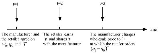
Figure 1.
Sequence of events.
Defining the information precision or quality as in Ha et al. [31,32], we can reflect the retailer’s skill at demand forecasting. After demand forecasting, the retailer obtains the posterior expectation of the market condition , which is the weighted average of and signal ([31,32,33]), . We see that when , , which means that the market demand is not improved.
3.2. Methodology
Under a Stackelberg game, by offering a wholesale price, the retailer decides the order quantity, which, in turn, determines the retail price. The optimal order quantity is the best response to the wholesale price. Hence, the subgame perfect equilibrium of this game can be found by backward induction.
Before demand forecasting, given any wholesale price set by the manufacturer, the retailer determines the order quantity to maximize the profit . Since , the first-order condition for , the optimal order quantity can be found to be . Also, the manufacturer determines to maximize the profit . Substituting the best response into yields the optimal initial wholesale price . Thus, the optimal order quantity is .
After demand forecasting, the manufacturer changes the wholesale price, and the retailer changes the prior order quantity. The transfer payment made by the retailer to the manufacturer is . Under such a transfer payment, the retailer purchases the committed order quantity at the initial wholesale price and the additional order quantity at the new wholesale price. This implies that the manufacturer provides the retailer with protection at the wholesale price: the retailer purchases the committed order quantity at the lowest price. For the manufacturer, the committed order quantity of the retailer is conducive to the production arrangements. The profits of the manufacturer and the retailer are as follows:
We also use the approach of backward induction to solve the optimal wholesale price and order quantity. (Lemma 1).
Lemma 1.
The optimal wholesale price and order quantity after information updating are
It is clear that the optimal wholesale price and order quantity are relevant to the posterior expectation of the market demand and the minimum order quantity before demand forecasting.
4. Analytical Results
In this section, we analyze the relationship between the optimal decisions (wholesale price, order quantity) and the market measure, the value of demand forecasting. Also, we investigate the effect of the retailer’s accuracy on the demand forecast.
4.1. Equilibrium Decisions
To show the effect of market variation on the optimal decisions of the manufacturer and the retailer, we define to measure the market variation. means that the market demand after the information updating is the same as before; () means that the retailer predicts that the demand is higher (lower) than previously expected, which represents a good (bad) market outlook.
In order to avoid trivial cases, we only consider the case that market status is not very bad, i.e., . Under such a condition, the wholesale price is no less than the production cost, and the minimum order quantity before demand forecasting can be ensured.
We next show the optimal wholesale price and order quantity under the market variation.
Proposition 1.
The optimal wholesale price under demand information updating is
Considering the retailer’s order decisions, the manufacturer offers a flexible wholesale price based on the market variation, which is shown in Figure 2. We make the following observations.
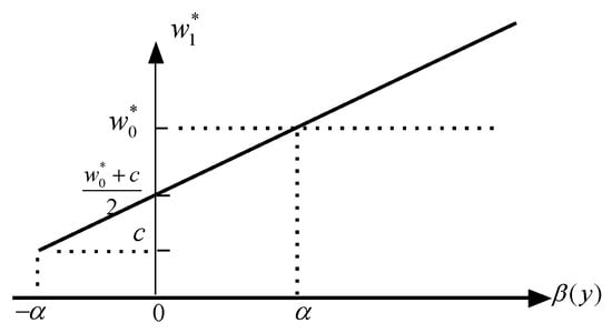
Figure 2.
Optimal wholesale price.
- (1)
- The wholesale price is increasing in the market variation measure. This means that as the market status improves, the manufacturer offers a higher wholesale price to the retailer, who can obtain a higher profit margin. Note that, at the lower bound of the measure of market variation, the wholesale price equals the production cost. This implies that if the market status is particularly bad, the manufacturer makes no profit.
- (2)
- The wholesale price may be higher or lower than the initial wholesale price. That is to say, depending on market demand variation, the manufacturer may offer a flexible wholesale price to ensure profit. Interestingly, only when the market status is good will the manufacturer increases the wholesale price. When the market status is average () or bad (), the manufacturer offers a wholesale price that is lower than the initial wholesale price to incentivize the retailer’s order. For a given production cost, the manufacturer’s profit margin decreases because of the average or bad market status. In order to ensure a higher profit margin, the manufacturer should pay more attention to the market status variation. Especially, when the market performance is average, the manufacturer should reconsider the popularization of innovative green products with consumers.
Proposition 2.
For a given wholesale price, the retailer’s optimal order and retail price after information updating are as follows for , where .
Proposition 2 shows that the optimal order after information updating is relevant to the minimum order and the variation of market status (see Figure 3). The main observations are as follows.
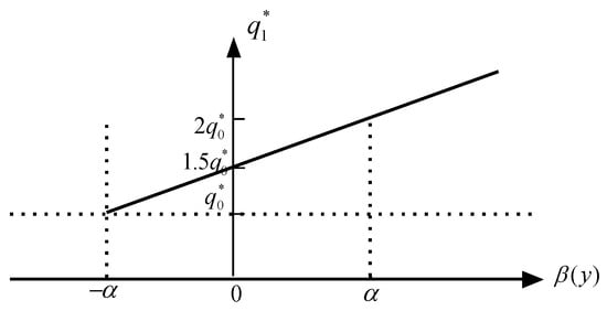
Figure 3.
Optimal order quantity.
- (1)
- As shown in Figure 3, the optimal order increases to match the market variation. As a response to the wholesale price, the retailer makes ordering decisions based on the market status. Considering the wholesale price based on the market variation, an interesting result is that the order quantity increases with the wholesale price. This is in contrast to the common assumption that the order quantity will decreases with the wholesale price under a Stackelberg game. The main reason is that the retailer is more sensitive to market variations than the manufacturer.
- (2)
- The additional order quantity increases to match the market variation . This implies that, as the market status improves, the retailer orders more. Moreover, the relationship between the ordering policy and the market variation shows an important managerial insight. Generally, the initial production quantity is typically 65–70% of the sales volume [34]. This mostly occurs when the market status is relatively good (), which is a special case in our analysis. Our results also include the cases and , which take place when the market status is average () and very good (), respectively. The results enrich the knowledge of initial production volume before demand updating and provide guidance for manufacturers to prepare order quantities that correspond to different market statuses.
- (3)
- The minimum order quantity can be ensured if the market status is larger than a lower bound. This implies that, if an innovative green product is not welcomed by consumers, the lower bound will be broken. Thus, the capacity reservation cannot be ensured if it would damage the manufacturer’s profit. Recall that the lower bound is also a condition that ensures that the wholesale price is not less than the production cost. Thus, only when the market status is not very bad can the dynamic contract be implemented.
Proposition 3.
(1) ; (2) .
Proposition 3 part (1) shows that the increasing rate of the retail price is larger than the wholesale price when the market status is better than expected. Part (2) means that the manufacturer obtains more profit margin than the retailer when the market status improves. As the market status improves, the retailer increases the order quantity, so the manufacturer makes more profit than the retailer. If the market status declines, the retailer decreases the order quantity and retail price, while the manufacturer decreases the wholesale price. However, the decreasing rate of the retail price is larger than that of the wholesale price when the market status is worse than expected. Thus, the profit margin decrease of the retailer is less than that of the manufacturer. Therefore, a flexible wholesale price strategy provides incentives for retailers. The better the market’s status, the more orders the retailer will make. Thus, the manufacturer can gain more to ensure sustainable profitability.
4.2. Value of Demand Forecasting and Sharing
In this subsection, we calculate the profits for the manufacturer and the retailer when there is or is not information updating. In order to avoid trivial cases, we still address the value of demand forecasting under the condition , i.e., the market status is not significantly worse than expected. The reason is that under our setting for the green product supply chain, there is no value to the green product if a few or no consumers purchase it.
Proposition 4.
(1) When,holds for.
(2) When,; when,.
(3) There exists, wheresuch thatwhen;when.
Proposition 4 describes the value of the demand forecast for the supply chain parties and supply chain. We come to the following conclusions.
- (1)
- When the cost of information sharing is less than an upper bound, demand forecasting and sharing are always beneficial for the manufacturer. As shown in Figure 4, when the cost of information sharing is not larger than the upper bound, the manufacturer always profits from demand forecast and sharing, even if the market outlook is worse than expected. The reasoning behind this is as follows. When the market status is better than expected, the manufacturer has a higher profit margin (Proposition 3). Combining this with a higher order, the manufacturer has a higher profit. When the market status is worse than expected, the manufacturer has a lower profit margin. With a lower order quantity, the manufacturer has a lower profit. Even in such a case, demand forecasting is still beneficial to the manufacturer. This is because the manufacturer, as a Stackelberg game leader who has the first-move advantage, can adjust the wholesale price to ensure profitability from shared demand information. Moreover, as the market demand increases, the manufacturer will gain more (Figure 4).
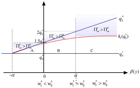 Figure 4. The manufacturer’s profit variation.
 - (2)
- The value of the demand forecast for the retailer is only affected by the market status. When the market demand is better than expected, the retailer benefits from the demand forecast; conversely, the retailer suffers a loss. The reasoning behind this is that when the market status is good, the retailer increases the order quantity and retail price. Since the increase rate of the retail price is larger than the increase rate of the wholesale price (Proposition 3), the retailer obtains a higher profit margin when the market status improves. Combining this with the increased quantity, the retailer can obtain more profit because of the demand forecast when the market status is good. Otherwise, the retailer lowers the order quantity and retail price. Since the decrease rate of the retail price is larger than the decrease of the wholesale price rate (Proposition 3), the retailer obtains a lower profit margin. With a decreasing order quantity, the retailer suffers a loss because of the demand forecast when the market status is bad. This implies that the retailer is more sensitive to the market variation than the manufacturer. Thus, it is necessary for the retailer to adopt some strategies to improve consumers’ awareness of the innovative green product.
- (3)
- As shown in Figure 5, by offering a flexible wholesale price, the retailer does not always benefit from the demand forecast, especially when the market status is worse than expected. The tuition behind is that a lower purchased volume of the green product leads to the retailer’s loss. Conversely, if the market status is better than expected, the retailer benefits from the demand forecast even if there is a higher wholesale price. The reasoning is that, when there is a higher wholesale price, the retailer increases the retail price. Thus, the joint effects of a higher profit margin and a higher selling volume ensure the retailer’s profit. Furthermore, as the market status improves (), the retailer will benefit more (Figure 5).
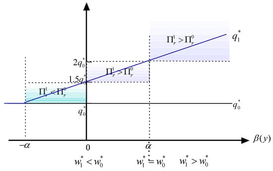 Figure 5. The retailer’s profit variation.
 - (4)
- Figure 6 illustrates that when the market outlook is worse than expected, the supply chain performance may improve. There is a threshold for market variation, below which the manufacturer and retailer both suffer losses because of the bad market outlook. Since the manufacturer benefits when the market status is bad, this may alleviate the supply chain profit loss arising from the retailer’s profit loss. Interestingly, when the market status is worse than expected but not very bad, the information updating contributes to supply chain profit increasing. That is to say, the gains of the manufacturer from information updating are larger than the losses of the retailer from the information updating when the market status is worse than expected.
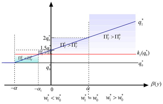 Figure 6. The supply chain profit variation.
4.3. The Effect of Forecast Accuracy
In this section, we analyze the effect of accuracy on the profits of the manufacturer, the retailer, and the supply chain. We consider the case where the market parameter is a normally distributed random variable with mean and variance , and the signal , where is independent of and . We make the following propositions.
Proposition 5.
(1) When,andhold.
(2) When,andhold.
Proposition 5 states that the demand forecast affects the wholesale price and the order quantity. Because of information sharing, the manufacturer knows not only the market status but also the accuracy of the demand forecast. Facing a good market outlook, the manufacturer sets a higher wholesale price when they know that the retailer has an accurate demand forecast. This means that more accurate demand information and a good market status help the manufacturer gain more profit margin. Conversely, when the market status is worse than expected, a retailer who is more skilled at demand forecasting decreases the manufacturer’s profit margin.
Since the retailer is clear about the demand forecast and the market status, they adjust the order quantity based on the market status. When facing a good (bad) market status, a higher accuracy of the demand forecast will increase (decrease) the order quantity. Therefore, the market status and the accuracy of the demand forecast jointly affect the wholesale price and order quantity adjustment. Next, we show how variations of the market status and the accuracy of the demand forecast affect the profits of the manufacturer, the retailer, and the supply chain.
Proposition 6.
(1) When,,,;
(2) When,,,.
Proposition 6 illustrates the impact of the market status and the accuracy of the demand forecast on the profits of firms and the entire supply chain. The results show that a higher accuracy of the demand forecast is not always beneficial for firms and the entire supply chain. The effects of the accuracy of the demand forecast are dependent on the market status. Facing a good market outlook, a higher accuracy of the demand forecast increases the profits of the manufacturer, the retailer, and the supply chain. The main reason is that higher information accuracy has more value when the market status is good. Since the manufacturer offers a higher wholesale price and the retailer makes more orders when the demand forecast is more accurate, the higher profit margin and higher number of orders contribute to higher firm and supply chain profit. However, when facing a bad market outlook, higher demand accuracy decreases the profits of the manufacturer, the retailer, and the supply chain. This indicates that manufacturers should not choose retailers with a higher capacity for demand forecasting. The market signal is a key issue for manufacturers when pricing innovative green products.
5. Numerical Examples
In this section, we provide numerical examples to show the impact of information accuracy. We first address the market variation under different cases, then address the impact of information accuracy on the decisions and profits. We finally address the cost of information sharing and the value of information forecasting and sharing for supply chain parties.
5.1. Measure of Market Variation
We consider the case where the market parameter is a normally distributed random variable with mean and variance , and the signal , where is independent of and . Since , can be expressed as , . For a realized signal , the measure of market variation can be written as . We fix and vary parameters , , and . The three cases are as follows: , and .
- (1)
- When , we have , , , , . Given , there exists a threshold such that holds for and for (see Figure 7a).
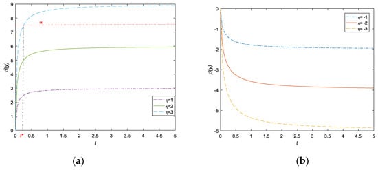 Figure 7. (a) varies in (); (b) varies in ().
Figure 7a shows the measure of market variation when the market is better than expected. In this case, the measure of market variation increases with the accuracy of the demand forecast. Also, means that the retailer has received a good signal from the market. This means that the relatively higher accuracy of the demand forecast () and a good signal contribute to the good market status. Otherwise, the lower accuracy of the demand forecast () and a good signal contribute to an average market status. With a realized signal , the accuracy of the demand forecast is a reference for the wholesale price adjustment.
- (1)
- When , we have , , , , . Given , we can see that (Figure 7b). Figure 7b shows the measure of the market variation when the market is worse than expected. means that the retailer has received a bad signal from the market. In this case, as the realized value decreases and the information accuracy increases, the market declines.
5.2. Effect of the Demand Forecast Accuracy
We next analyze the impact of the demand forecast accuracy on the decisions and profits in the abovementioned cases.
Figure 8a–d show the impacts of the accuracy of the demand forecast on the wholesale price and order quantity as well as the profits of the manufacturer and the retailer when the market is good. Our main observations are as follows.
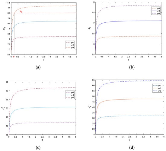
Figure 8.
(a) Wholesale price varies in (); (b) order quantity varies in (); (c) manufacturer’s profit varies in (, ); (d) retailer’s profit varies in (, ).
- (1)
- There exists a threshold of the accuracy of the demand forecast such that the manufacturer adjusts the wholesale price. For a given realized signal , whether the market status is good or average depends on whether the forecast accuracy is higher or lower than the threshold of forecast accuracy. Hence, when the accuracy of the demand forecast is lower (higher) than the threshold, the manufacturer offers a lower (higher) wholesale price than the initial wholesale price after information updating. Moreover, when the accuracy of the demand forecast is higher than the threshold, the impact of information accuracy on the wholesale price is smaller than when the accuracy of the demand forecast is lower than the threshold. As shown in Figure 8a, the wholesale price tends to be stable as the information accuracy increases. Also, as the positive market signal () increases, the wholesale price becomes higher. Interestingly, for the manufacturer, higher information accuracy and a good market signal do not increase the wholesale price by much, but a lower information accuracy together with a good market signal increase the wholesale price by a lot. Thus, for a given market signal, the manufacturer can determine to increase or decrease the wholesale price according to the demand forecast.
- (2)
- The retailer always achieves an order quantity that is larger than the minimum order quantity. Similar observations can be seen in Figure 8b. The order quantity tends to be stable as the information accuracy increases. Also, as the positive market signal () increases, the order quantity becomes larger. Interestingly, higher information accuracy and a good market signal do not increase the order quantity by much, but lower information accuracy together with a good market signal increases the order quantity by a lot.
- (3)
- The profits of the manufacturer and the retailer are higher after demand forecasting and sharing than before. This implies that the effect of demand forecasting and sharing is positive when the market is better than expected. Furthermore, the profits of the manufacturer and retailer increase with the accuracy of the demand forecast. Both the manufacturer and the retailer benefit from having a more accurate idea of the market demand. However, the high accuracy of the demand forecast does not always increase the profits of the supplier and the retailer. Thus, when the market status is good, a higher information accuracy does not increase profits by much, but a lower information accuracy does. This indicates that manufacturers need to seek out more accurate demand information.
Figure 9a,b show the impacts of the accuracy of the demand forecast on the wholesale price, order quantity, and profits of the manufacturer and the retailer when the market is bad. Some main observations are as follows.
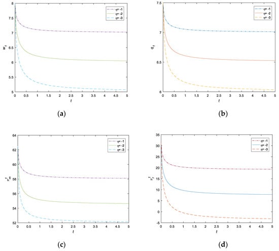
Figure 9.
(a) Wholesale price varies in (); (b) order quantity varies in (); (c) manufacturer’s profit in (, ); (d) retailer’s profit in (, ).
- (1)
- Both the wholesale price and the retailer decrease with the accuracy of the demand forecast. As the situation deteriorates, the manufacturer and the retailer reduce their wholesale price and order quantity, respectively. That is to say, as the market signal becomes worse, the manufacturer lowers the wholesale price further. In other words, the manufacturer incentivizes the retailer to increase the order quantity to ensure profit. Unfortunately, the retailer wants to order less due to the bad market signal. Moreover, the positive effect of the lower wholesale price incentive outweighs the negative effect of a lower order, so the retailer always makes an order that is larger than the minimum order quantity.
The manufacturer’s profit is higher after the demand forecasting and sharing than before, and increases with the accuracy of the demand forecast. When the accuracy of the demand forecast is relatively low, the manufacturer’s profit is negatively affected. In contrast, high accuracy of the demand forecast does not always damage the manufacturer. Additionally, as the market demand signal becomes worse, the manufacturer’s profit decreases.
The retailer’s profit decreases sharply when the information accuracy is relatively low. This implies that when the market status is bad, the manufacturer prefers that the retailer does not forecast demand. Thus, the retailer can make an order based on the expectation of the market demand. In return, the manufacturer offers a wholesale price based on the expectation of the market demand.
5.3. The Value of Demand Forecasting and Sharing
Figure 10 shows that the upper bound of the information sharing cost increases (decreases) in accuracy when the market status is better (worse) than expected. When the market status is better than expected, higher information accuracy implies higher information quality. The manufacturer is likely to pay more to acquire the demand information from the retailer. Thus, the upper bound of the information-sharing cost is increasing. If the cost of information sharing is lower than the minimum, the manufacturer always benefits from demand forecasting and sharing. Conversely, when the market is worse than expected, higher information accuracy does not mean higher information quality. The manufacturer benefits only when the cost of information sharing is sufficiently low. For example, when , the highest cost of information sharing is about 7. Next, we show the value of demand forecasting and sharing for the manufacturer and retailer, respectively, with different costs of information sharing.
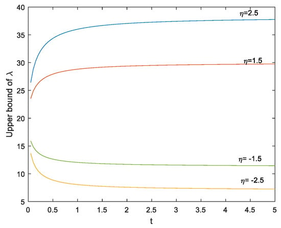
Figure 10.
The upper bound of information-sharing cost ().
Figure 11a,b shows the value of the demand forecast for the manufacturer and the retailer when the market status is better than expected. We make two main observations.
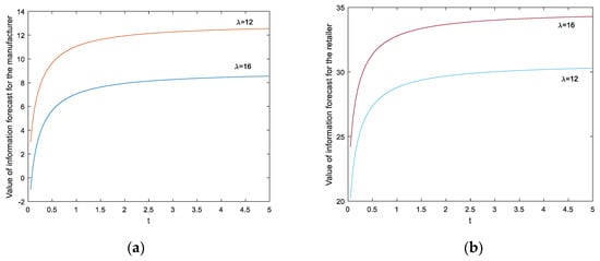
Figure 11.
(a) Value of demand forecast for the manufacturer (); (b) value of demand forecast for the retailer ().
- (1)
- The value of the demand forecast increases with the information accuracy. This implies that high information accuracy does not help the manufacturer or retailer very much.
- (2)
- Reducing the cost of information sharing is beneficial to the manufacturer. Thus, the manufacturer should evaluate the upper bound of the information-sharing cost and make an agreement on the cost so as to ensure benefit.
Figure 12a,b shows the value of the demand forecast for the manufacturer and the retailer when the market status is worse than expected. We make two main observations.
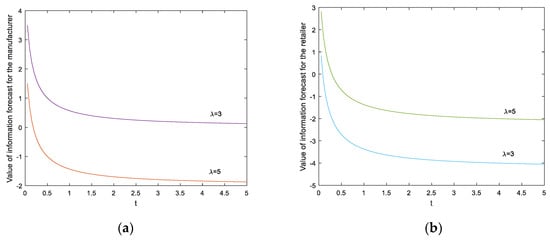
Figure 12.
(a) Value of demand forecast for the manufacturer (); (b) value of demand forecast for the retailer ().
- (1)
- The value of the demand forecast increases with the information accuracy. In contrast to the previous situation, high information accuracy decreases the value of information sharing for the manufacturer and the retailer. The retailer, especially, may suffer from demand forecasting; a higher information accuracy incurs a higher loss. This result complements the theoretical results in Proposition 4. Meanwhile, the manufacturer should be careful about agreeing to the cost of information sharing. A lower cost of information may decrease the value of demand forecasting and sharing for the manufacturer.
- (2)
- Reducing the cost of information sharing is also beneficial to the manufacturer when the market status is worse than expected. However, the manufacturer should be careful about agreeing to the cost of information sharing. A lower cost of information may decrease the value of demand forecasting and sharing for the manufacturer.
In summary, the numerical examples provide additional managerial insights to supplement the theoretical results. When the information accuracy is lower, the wholesale price and order quantity vary widely; the profits of the manufacturer and the retailer vary widely as well. Specifically, when the market status is good (bad), the wholesale price and the order quantity increase (decrease) sharply with the information accuracy; the profits of the manufacturer and the retailer increase (decrease) sharply with the information accuracy. The manufacturer and retailer do not need to prioritize high information accuracy, no matter if the market status is good or bad. Additionally, launching demand forecasting and sharing is not necessary when the retailer has received a bad market signal. The right pricing strategy for innovative green products for the manufacturer is to match the price of regular products, and the right ordering strategy for the retailer is to purchase the minimum order quantity as the final order quantity. Furthermore, the manufacturer should evaluate the upper bound of the information-sharing cost and make an agreement with the retailer on a cost of information sharing that is not higher than the upper bound to ensure benefit.
6. Discussion
In this section, we discuss our main findings and consider a possible application in the green supply chain.
6.1. Decisions and Profits
In Section 4, Propositions 1 and 2 gave the optimal wholesale price and order quantity in the dynamic contract under demand forecasting and sharing. The flexible wholesale price of the innovative green product based on demand variation provides sufficient incentives for the retailer to adopt an optimal order strategy. Interestingly, the retailer’s order quantity increases with the wholesale price. The main reason is that the market variation affects the order strategy more than the wholesale price and a good market status increases the retailer’s order. Also, Proposition 3 shows that the manufacturer obtains a greater profit margin than the retailer when the market status improves. When the market status worsens, the retailer decreases the order quantity and retail price, while the manufacturer decreases the wholesale price. Thus, the profit margin decrease of the retailer is less than that of the manufacturer. With a lower order quantity, the retailer suffers a lower loss than the manufacturer.
Therefore, a dynamic contract can incentivize a retailer to sell innovative green products to consumers. The better the market status, the more orders the retailer will make. Thus, the manufacturer can gain more and ensure sustainable profits.
6.2. Value of Demand Forecasting
Since the retailer is closer to the market, information sharing incurs a cost that will be paid by the manufacturer. Thus, the value of demand forecasting and sharing may be affected by the cost of information sharing. Surprisingly, when the cost of information sharing is no more than an upper bound, the value of demand forecasting and sharing is always beneficial to the manufacturer no matter if the market demand status is good or bad. In practice, a manufacturer who launches an innovative green product can generally afford the cost of information sharing. However, the value of demand forecasting for the retailer is only affected by the market status. When the market demand is better than expected, the retailer benefits from the demand forecast; conversely, the retailer suffers a loss.
6.3. Forecast Accuracy and Capability
Higher (lower) information accuracy implies the higher (lower) capability of the demand forecast (e.g., [25]). Previous literature on the green supply chain has seldom investigated the forecasting ability’s impact on the decision-making and profits of the parties and supply chain. Our results show that a more accurate demand forecast can help with making better decisions. Combining the market status impact and information accuracy, decision makers can understand how their profits vary in two dimensions. Our numerical analysis shows that a higher information accuracy may not increase profits for either the manufacturer or the retailer, even if the market status is better than expected.
6.4. Managerial Insights and a Possible Application
Our analytical and numerical results provide some insights into supply chain sustainability for managers.
For an innovative green product manufacturer, maintaining economic returns while doing good for society and the environment is very important. Thus, knowing the market demand and setting an appropriate price for innovative products are main tasks for the manufacturer. (1) Analytical results provide decision support for wholesale pricing when the market demand varies. For example, when the market is good, offering a higher wholesale price is a good strategy for a manufacturer. However, when the market demand is worse than expected, a lower wholesale price is a good strategy. Numerical examples show different wholesale price strategies under three different market statuses (good, average, bad). This might lead to some implications for innovative green product firms. (2) Since the retailer has the advantage of market demand, the manufacturer should consider the cost of information sharing with a retailer. Demand forecast sharing is beneficial to the manufacturer if the cost of information sharing is lower than the upper bound (as shown in Proposition 4). The manufacturer should evaluate the upper bound of the information-sharing cost and make an agreement with the retailer about the cost. (3) In order to ensure economic returns for developing an innovative green product, the manufacturer can adopt a dynamic contract. The contract specifies an initial wholesale price, a minimum order quantity, a demand sharing agreement, and a decisions adjustment agreement. The committed minimum order quantity helps the green product firm (manufacturer) build a reserve capacity, which reduces the manufacturer’s risk of a mismatch between production and demand.
For the retailer, knowing more about the market demand variation helps with making better marketing strategies (order and price). The value of demand forecasting is largely affected by the market status. If the market demand is worse than expected, the retailer will not benefit from demand forecasting. Thus, one important managerial insight for the retailer is that the retailer can make some efforts to help consumers improve their awareness of green products and change their consumption patterns.
For both the manufacturer and the retailer, the accuracy of the demand forecast is also important. However, the manufacturer should not prefer high accuracy of demand because this does not improve the profits of the manufacturer and retailer when the market demand is better than expected, and high accuracy of demand lowers the manufacturer’s profit when the market demand is worse than expected.
In summary, a system for understanding market demand forecasting and sharing can lead to better solutions, allowing supply chain parties to implement foundational practices for sustainable supply chain development.
The findings and managerial implications discussed above can be applied to the innovative green product supply chain. For example, in the fashion industry, a firm plans to launch a program to produce innovative green products (e.g., [7]). Before knowing more accurate market demand, the manufacturer offers an initial wholesale price (e.g., the price of the regular product) and requires a minimum order quantity to ensure the reserve capacity. Also, the manufacturer and the retailer make an agreement on the cost of information sharing and price/order adjustment based on shared demand information. When demand signals are acquired, the manufacturer adopts a pricing strategy according to the shared information and market status, so as to make operations sustainable. The retailer also adopts order strategies in response to the market variation and wholesale price variation, thus ensuring profitability.
7. Conclusions
Sustainable supply chain management has become a growing concern in the face of limited environmental resources and a growing population [2]. In order to obtain economic returns for sustainable innovation of green products while considering the social and environmental impacts, making appropriate pricing/order strategies and forecasting the market demand are key issues. This paper investigates pricing and ordering strategies for innovative green product under demand forecasting and sharing. We formulate this problem using a Stackelberg game and propose a dynamic contract.
By analyzing the equilibrium strategies of the two parties, we show that the manufacturer offers a flexible wholesale price for the green product that is largely dependent on the market status variation. Also, the retailer’s order quantity increases with the wholesale price, which seems to contradict common knowledge. As the market improves, the manufacturer obtains more profit margin than the retailer; as the market status worsens, the manufacturer suffers a greater loss of profit margin than the retailer. The theoretical results and numerical results provide different wholesale pricing and ordering strategies under different market statuses (good, average, bad). Previous work has not investigated the effect of market variation on decision-making. By investigating the impact of demand forecasting and sharing, we show that when the cost of information sharing is smaller than an upper bound, demand forecasting and sharing are always beneficial for the manufacturer. However, the value of demand forecasting and sharing for the retailer is significantly affected by variations in the market status. The upper bound of the information-sharing cost gives a reference for the manufacturer to make an agreement on the cost of information sharing. Thus, the manufacturer always knows the value of demand forecasting and sharing. Previous work has seldom considered the cost of information sharing between supply chain parties. By addressing the impact of information accuracy, we show that high information accuracy may not increase the profits of either the manufacturer or the retailer, even if the market status is better than expected. Thus, one important managerial insight for the manufacturer and the retailer to consider is that they should not prioritize high information accuracy. Previous work has not considered the impact of information accuracy on decisions and profits. Our interesting and important findings shed light on how a manufacturer can set the right price for innovative green products under different market demand. Also, these findings will help retailers to set better marketing strategies under different market statuses.
Our study complements previous work on the pricing of green products and on demand forecasting and information sharing in a green supply chain. Moreover, it gives managerial insights for manufacturers and retailers to put in practice, especially when the market demand varies. Finally, a dynamic contract that allows for adjustments of the wholesale price and the order quantity for the supply chain parties is proposed to achieve the sustainable development of the supply chain.
Future research can extend the analysis of this paper in several directions. First, a direct extension of the present findings involves assuming that the retailer is risk-averse. Attitude to risk affects the demand forecast, which, in turn, affects the pricing strategies and ordering policy. Second, future research should take into consideration the public signal’s effect on market demand. Public signals of the market, such as media buzz and green innovation policy, have a major effect on consumers’ awareness of green products, which in turn influence consumer’s behavior.
Author Contributions
All of the authors contributed significantly to the completion of this manuscript. Y.F. and J.Y. developed the overall idea and models, and performed the investigation. X.W. contributed to the theoretical verifications, discussion of results, and numerical studies. Y.F. and X.W. wrote the manuscript; X.W. and J.Y. revised the manuscript. All authors have read and agreed to the published version of the manuscript.
Funding
This work was supported by the National Natural Science Foundation of China (grant number 71501161), the Ministry of Education, Humanities and Social Science Planning Funds (grant number 16YJC630026), the Fundamental Research Funds for the Central University (grant number skqy201768), the Young Teachers Fund for the Central University (grant number 2018NQN29), and Science and Technology Development of Sichuan Province of China (grant numbers 2019JDR0169, 2019JDR0210).
Conflicts of Interest
The authors declare no conflict of interest.
Appendix A
Proof of Lemma 1.
Since , . It is noted that . Thus, given a wholesale price, the retailer’s optimal response solves , i.e., . Substituting into the equation of , we obtain . It is noted that and . Let and we get the optimal wholesale price . Substituting into , we obtain . □
Proof of Proposition 1.
From Lemma 1 and Equation (2), we have . Thus can be written as . □
Proof of Proposition 2.
From Lemma 1 and Equation (3), we have . Then we can obtain . □
Lemma 2.
,;,.
Proof of Lemma 2.
With the initial agreement, the manufacturer’s profit function is
□
After information updating, the manufacturer’s profit functions are:
Proof of Proposition 3.
Since and , the optimal retailer price is . Thus, we have , and since , we have . Thus, we have . We also have . Thus, it holds that . □
Proof of Proposition 4.
(1)
From Lemma 2, we have
By Proposition 1, we have . Thus, . Let , and be the solution of the equation . We have . This implies that, if , holds.
We then prove that always holds when . Since , we have . Since we know that when , holds. Letting , we find that when , holds for .
(2)
Combining with Lemma 2, we discover that
If , ; If , .
If , holds, it holds that
This implies that , . The upper bound of the information-sharing cost can be written as . From Proposition 1, we know that for . Thus, , which does not satisfy the condition () for , holds. Therefore, when .
(3)
Using the formulas , , we have . Letting , and be the solution of the equation , we can obtain . Thus, when , ; , . Since , let ; we then have . There exists that satisfies the equation . Because is increasing in , we know that when , holds, and when , holds. □
Lemma 3.
holds for;holds for.
Lemma 3 shows the monotonicity of the measure of the market status variation. With a good market outlook, higher information accuracy increases the value of information updating. Conversely, with a good market outlook, higher information accuracy decreases the value of information updating.
Proof of Lemma 3.
Since , can be expressed as , . We have . For a realized signal , we have . is equivalent to , so we know that holds for ; holds for . □
Proof of Proposition 5.
Since (Proposition 1), it holds that . From Lemma 3, we know that for , and for . Since , it holds that . Combining with Lemma 3, we can obtain , for , and for . □
Proof of Proposition 6.
When , , and hold. Combining and , we have . When , , and hold. Combining and , we have
Therefore, when , , , . When , , , . □
References
- Zhu, W.; He, Y. Green product design in supply chains under competition. Eur. J. Oper. Res. 2017, 258, 165–180. [Google Scholar] [CrossRef]
- Rebs, T.; Brandenburg, M.; Seuring, S. System dynamics modeling for sustainable supply chain management: A literature review and systems thinking approach. J. Clean. Prod. 2019, 208, 1265–1280. [Google Scholar] [CrossRef]
- Seuring, S.; Müller, M. From a literature review to a conceptual framework for sustainable supply chain management. J. Clean. Prod. 2008, 16, 1699–1710. [Google Scholar] [CrossRef]
- Choi, T.M. Pricing and branding for remanufactured fashion products. J. Clean. Prod. 2017, 165, 1385–1394. [Google Scholar] [CrossRef]
- Clancy, H. How She Leads: Letitia Webster. 2004. Available online: https://www.greenbiz.com/blog/2014/08/14/how-she-leads-letitia-webster-vf (accessed on 14 August 2014).
- Very, S. The Rise of Eco-friendly Consumer Products Puts Pressure on P&G. Bloomberg. Available online: https://www.bloomberg.com/news/articles/2016-10-04/p-g-under-pressure-to-make-a-deal-as-eco-friendly-products-surge (accessed on 4 October 2016).
- Shen, B.; Choi, T.M.; Chan, H.L. Selling green first or not? A Bayesian analysis with service levels and environmental impact considerations in the Big Data Era. Technol. Forecast. Soc. Chang. 2017, 144, 412–420. [Google Scholar] [CrossRef]
- Pagell, M.; Shevchenko, A. Why research in sustainable supply chain management should have no future. J. Supply Chain Manag. 2014, 50, 44–55. [Google Scholar] [CrossRef]
- Gosling, J.; Jia, F.; Gong, Y.; Brown, S. The role of supply chain leadership in the learning of sustainable practice: Toward an integrated framework. J. Clean. Prod. 2017, 140, 239–250. [Google Scholar] [CrossRef]
- Zimon, D.; Tyan, J.; Sroufe, R. Implementing Sustainable Supply Chain Management: Reactive, Cooperative, and Dynamic Models. Sustainability 2019, 11, 7227. [Google Scholar] [CrossRef]
- Li, Y.; Su, Z.; Liu, Y. Can strategic flexibility help firms profit from product innovation? Technovation 2010, 30, 300–309. [Google Scholar]
- Lin, R.J.; Tan, K.H.; Geng, Y. Market demand, green product innovation, and firm performance: Evidence from Vietnam motorcycle industry. J. Clean. Prod. 2013, 40, 101–107. [Google Scholar] [CrossRef]
- Fonseca, L.; Domingues, J.; Pereira, M.; Martins, F.; Zimon, D. Assessment of circular economy within Portuguese organizations. Sustainability 2018, 10, 2521. [Google Scholar] [CrossRef]
- Özer, Ö.; Wei, W. Strategic commitments for an optimal capacity decision under asymmetric forecast information. Manag. Sci. 2006, 52, 1238–1257. [Google Scholar] [CrossRef]
- Liu, P.; Yi, S.P. Pricing policies of green supply chain considering targeted advertising and product green degree in the big data environment. J. Clean. Prod. 2017, 164, 1614–1622. [Google Scholar] [CrossRef]
- Hong, Z.; Wang, H.; Yu, Y. Green product pricing with non-green product reference. Transp. Res. Part E Logist. Transp. Rev. 2018, 115, 1–15. [Google Scholar] [CrossRef]
- Hong, Z.; Guo, X. Green product supply chain contracts considering environmental responsibilities. Omega 2019, 83, 155–166. [Google Scholar] [CrossRef]
- Rahmani, K.; Yavari, M. Pricing policies for a dual-channel green supply chain under demand disruptions. Comput. Ind. Eng. 2019, 127, 493–510. [Google Scholar] [CrossRef]
- Zhang, T.; Choi, T.M.; Zhu, X. Optimal green product’s pricing and level of sustainability in supply chains: Effects of information and coordination. Ann. Oper. Res. 2018, 1–26. [Google Scholar] [CrossRef]
- Shu, Y.; Dai, Y.; Ma, Z. Pricing decisions in closed-loop supply chains with peer-induced fairness concerns. Sustainability 2019, 11, 5071. [Google Scholar] [CrossRef]
- Zhang, H.; Zhang, Z.; Pu, X.; Li, Y. Green manufacturing strategy considering Retailers’ fairness concerns. Sustainability 2019, 11, 4646. [Google Scholar] [CrossRef]
- Chintapalli, P.; Disney, S.M.; Tang, C.S. Coordinating supply chains via advance-order discounts, minimum order quantities, and delegations. Prod. Oper. Manag. 2017, 26, 2175–2186. [Google Scholar] [CrossRef]
- Özer, Ö.; Uncu, O.; Wei, W. Selling to the “newsvendor” with a forecast update: Analysis of a dual purchase contract. Eur. J. Oper. Res. 2007, 182, 1150–1176. [Google Scholar] [CrossRef]
- Taylor, T.A. Sale timing in a supply chain: When to sell to the retailer. Manuf. Serv. Oper. Manag. 2006, 8, 23–42. [Google Scholar] [CrossRef]
- Taylor, T.A.; Xiao, W. Does a manufacturer benefit from selling to a better-forecasting retailer? Manag. Sci. 2010, 56, 1584–1598. [Google Scholar] [CrossRef]
- Miyaoka, J.; Hausman, W.H. How improved forecasts can degrade decentralized supply chains. Manuf. Serv. Oper. Manag. 2008, 10, 547–562. [Google Scholar] [CrossRef]
- Amornpetchkul, T.; Duenyas, I.; Şahin, Ö. Mechanisms to induce buyer forecasting: Do suppliers always benefit from better forecasting? Prod. Oper. Manag. 2015, 24, 1724–1749. [Google Scholar] [CrossRef]
- Vives, X. Oligopoly Pricing; MIT Press: Cambridge, MA, USA, 1999. [Google Scholar]
- Shang, W.; Ha, A.Y.; Tong, S. Information sharing in a supply chain with a common retailer. Manag. Sci. 2015, 62, 245–263. [Google Scholar] [CrossRef]
- Chen, F.; Lai, G.; Xiao, W. Provision of incentives for information acquisition: Forecast-based contracts vs. menus of linear contracts. Manag. Sci. 2016, 62, 1899–1914. [Google Scholar] [CrossRef]
- Ha, A.Y.; Tong, S.; Zhang, H. Sharing demand information in competing supply chains with production diseconomies. Manag. Sci. 2011, 57, 566–581. [Google Scholar] [CrossRef]
- Ha, A.Y.; Tian, Q.; Tong, S. Information sharing in competing supply chains with production cost reduction. Manuf. Serv. Oper. Manag. 2017, 19, 246–262. [Google Scholar] [CrossRef]
- Ericson, W.A. A note on the posterior mean of a population mean. J. R. Stat. Soc. 1969, 31, 332–334. [Google Scholar] [CrossRef]
- Hellen, O.Y. How to Forecast Demand for New Products. Available online: https://blog.arkieva.com/demand-forecasting-new-products/ (accessed on 23 January 2019).
© 2020 by the authors. Licensee MDPI, Basel, Switzerland. This article is an open access article distributed under the terms and conditions of the Creative Commons Attribution (CC BY) license (http://creativecommons.org/licenses/by/4.0/).