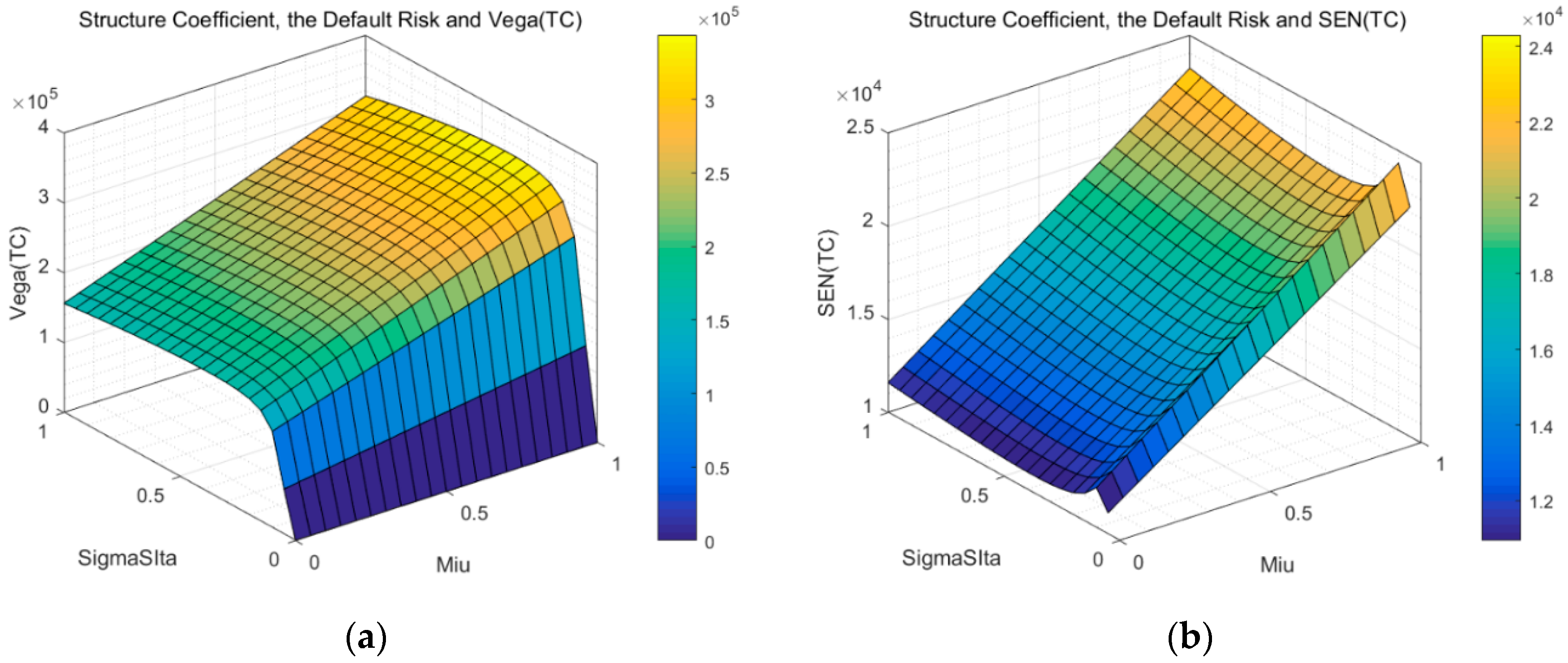
Article

Cash Salary, Inside Equity, or Inside Debt?—The Determinants and Optimal Value of Compensation Structure in a Long-term Incentive Model of Banks

1
School of Management, Harbin Institute of Technology, Harbin City 150000, China
2
School of Business, Singapore University of Social Sciences, Singapore 599494, Singapore
*
Author to whom correspondence should be addressed.
Sustainability 2020, 12(2), 666; https://doi.org/10.3390/su12020666
Submission received: 24 December 2019 / Revised: 15 January 2020 / Accepted: 16 January 2020 / Published: 16 January 2020
(This article belongs to the Section Economic and Business Aspects of Sustainability)

Abstract

:
The design and optimization of executive compensation structure to reduce the risk-taking of banks is one of the core topics of corporate governance theory. Especially after the 2008 global financial crisis, due to the characteristics of banks, such as systemic risk, this issue has become more important. However, though widely concerned, the determinants and design principles of compensation are not thoroughly understood. Based on our previous work, the setup of a banker’s long-term total compensation model, we continue our research by setting up a theoretical model between total compensation, bank default risk, and the structure coefficient by simulating the result using data from Wells Fargo and Co. to draw the function image. We are the first to find out the determinants of structure, that is, the working time, current age, and tenure. What is more important is that we find that increasing the weight inside debt in the total compensation is not only helpful for the reduction of the bank’s default risk, but also an increase of the banker’s total compensation. We also illustrate the influence of a number of periods. We expect our findings to offer help regarding the formulation of policies for pay contracts.

1. Introduction

In 1976, Jensen and Meckling [1] first published their article about executive compensation. Since then, elucidating how to design the pay contract and optimize the structure of banker’s compensation is becoming more and more prevalent in corporate governance theory. Particularly, since the occurrence of the 2007–2009 financial depression, the relation between compensation and bank risk-taking due to the systematic risk of a bank is increasingly significant. However, though widely focused, the determinants and design principles of pay contracts are not thoroughly understood.
Figure 1 summarizes the schematic diagram of the research framework of our study. We define the total compensation as the sum of cash salary, inside equity, and inside debt. At the same time, the structure coefficient in our paper stands for the weight of inside debt in total compensation, where “inside equity” is the equity-based compensation paid in the form of restricted stock, stock options, and other instruments, of which the value lies in the equity returns in the future. Per Jensen and Meckling [1], “inside debt” is defined as benefit pensions and deferred compensation. The determinants of the structure coefficient contain the working time, current age, and tenure of the banker. The object of our research is to find out the optimal level of the structure coefficient to decreased the bank’s default risk and to increase the banker’s total compensation.
Many researchers have studied structure design in various aspects. Agnieszka and Anna (2019) [2] concluded that the model of a credit cooperative movement, such as the one adopted in Poland, requires the implementation of a couple of basic changes. Tang (2016) [3] shows that option-like pay is more likely to maintain incentive effects. Shan and Walter (2016) [4] offer the fundamental building blocks for designing executive remuneration systems in public firms. Kline et al. (2017) [5] have found an inverse relationship between stock ownership and risk-adjusted performance. Fried (2011) [6] also puts forward a mechanism that ties executive pay to aggregate shareholder value. Dutcher (2018) [7] and Conyon (2006) [8] have shown that boards and compensation committees have become more independent over time. Canyon (2009) [9] has found out that the amount of inside equity is greater in firms that use consultants. Burak (2018) [10] suggests that those who are discontent with extremely high pay may be reconciled with support for pay for performance. Bebchuk et al. (2002) [11] highlight the significance of the design of executive compensation generally. Banghoj et al. (2010) [12] have examined what determines executive compensation in privately held firms.
Other aspects of compensation structure influence a bank’s situation. For instance, Milidonis et al. [13] have identified a significant and negative relationship between chief executive officer (CEO) inside debt holdings and risk-taking behavior. Deng et al. [14] showed that deferring CEO compensation significantly reduces bank risk-taking in an emerging market. Chen and Fan [15] investigated the effects of a borrowing firm’s CEO inside debt holdings on the structure of the firm’s syndicated loans. Bhandari et al. [16] linked debt-like compensation to financial analyst behavior. The results reported by Sheikh [16] suggest that market competition significantly influences the effect of CEO inside debt and corporate risk-taking. Li et al. [17] provided an inside debt metric that is conceptually superior to previously used metrics. Li and Zhang [18] stated that firms with a higher ratio of female directors tend to have a larger proportion of short-maturity debt. Li et al. [19] found that when a CEO holds a large amount of inside debt, a firm is less likely to issue convertibles than straight debt. Merton (1974) [20] used a framework to describe pay. Boyle and Scott (2006) [21] found sufficient conditions about option functions.
When it comes to bank risk, the measure and distinction of different kinds of risk is crucial in the following summary. First, the last financial crisis highlighted the problem of liquidity management and credit risk. Indeed, Galletta and Mazzù (2019) [22] made a liquidity mismatch index based on the loan-to-deposit ratio of a European sample. Moreover, Pelizzon et al. (2016) [23] and Diamond (1991) [24] investigated the dynamic relation between credit risk and liquidity, finding that the long-term refinancing operations weakened the sensitivity of market makers’ liquidity provision to credit risk, highlighting the importance of funding liquidity measures as determinants of market liquidity. Furthermore, Imbierowicz and Rauch (2014) [25] investigated the relationship between the two major sources of bank default risk, namely, liquidity risk and credit risk, and how this relationship influences banks’ probabilities of default (PD).
Overall, our study is important for understanding financial stability. Specifically, Abad-Segura et al. [26] raised the obligation of companies to corporate social responsibility from a sustainability approach. We initiated this research by modeling a structure coefficient with respect to the bank default risk, basing our findings on our previous work (Ma et al., 2020 [27]), where we investigated a banker’s long-term compensation. We demonstrated the relationship of the structure coefficient of total compensation with the bank’s default risk by formulating a particular formula. After setting the model of structure coefficient and the default risk, we simulated the result using data from Wells Fargo and Co. to draw the function image to identify additional features. We used CEO compensation and U.S. bank accounting data from the ExecuComp and BvD Orbis databases.
Firstly, we find an optimal situation about the structure coefficient to reduce a bank’s default risk, that is, increasing the weight of inside debt in total compensation is not only helpful for the reduction of the bank’s default risk, but also the increase of banker’s total compensation. At the same time, we are the first to find out the determinants of structure, that is, the working time, current age, and tenure. Last but not the least, we also illustrate the influence of a number of periods. We expect our findings to offer help regarding the formulation of policies for pay contracts.
The remainder of this paper is organized as follows. We create a model of structure coefficient with respect to bank default risk, basing our model on the long-term total compensation presented in Section 2. We characterize the function of structure function and bank default risk and then we analyze the determinants and other natures of functions and related indicators, such as the total compensation vega, V e g a T C , the sensitivity of total compensation, S E N T C and the number of periods, λ , in Section 3 (also shown in Figure 1). Then, we draw a fitting graph using the Wells Fargo and Co. data in Section 4. The last section concludes the paper.

2. Materials and Methods

Firstly, Table 1 summarizes the notations and definitions in our model.

2.1. Model Assumptions

To develop the banker’s compensation model, we assumed the following:
Assumptions 1–7 are the corresponding assumptions of (a)–(g) of Black and Scholes (1973) [28].
Assumption 8 is the total compensation, T C , during the executives’ tenure, which consists of three parts, namely, cash salary, C S , inside equity, I E , and inside debt, I D :
T C = C S + I E + I D
Assumption 9: Executives of banks die at exactly the age of 120 years.
Assumption 10: The inside equity frequency is the same as that of the inside debt.
Assumption 11: The interval at which each executive receives their inside equity is the same.
Assumption 12: Liquidation is costless and absolute priority holds.
Assumption 13: The banker’s compensation is so small relative to the net assets that its effect on the net asset dynamics can be ignored.
Assumption 14 is that the bank is operating normally, and that no bankruptcy occurs during the banker’s tenure.

2.2. The Long-Term Incentive Model of Banks

In our previous work, a long-term incentive model for compensation has been established. We will first briefly list the formulae used in this article and further explore the nature of the compensation structure based on this. See Ma et al. for further information in this regard (2020) [27].

2.2.1. Call Option and Total Compensation Value

If C ( ,   K C ) is the current value of a call option on the bank with strike price K C , then we obtain the following:
C ( ,   K C ) = E [ e x p ( r ) m a x ( E q ( ) E q ( 0 ) K C , 0 ) ] = N x ( d 1 ( ) ) K C e x p ( r ) N x ( d 2 ( ) )
where N x ( x ) = x n x ( t ) d t is the standard cumulative normal distribution and n x ( x ) = 1 2 π e x p ( x 2 2 ) is the standard normal density:
d 1 ( ) = 1 σ θ [ I n ( 1 K C ) + ( 1 2 σ θ 2 + r ) ]
d 2 ( ) = d 1 ( ) σ θ
Thus, C ( ,   K C ) is -maturity European call option on E q ( ) E q ( 0 ) with strike price K C , and r is the risk-free rate.
The value of total compensation with λ payout periods on [ K A ,   S ] is as follows:
T C = ( 1 + μ ) ( λ ω E q ( 0 ) C ( Δ , 1 ) + C S )
where μ = M S κ n = m a x ( 0 , R A ) K A p ( n ) ( 1 + d ) n , κ = S K + A = λ Δ , C ( Δ , 1 ) is the call option price from Equation (15), ω is the fraction of profits paid out as compensation, and E q ( 0 ) is the initial net asset value.

2.2.2. The Vega and Sensitivity of Total Compensation

We denote V e g a T C and S E N T C as the vega and sensitivity of total compensation, respectively. From Corollaries 2 and 3 and Proposition 1 (outlined further below), we also have the following:
V e g a T C = ( 1 + μ ) λ ω E q ( 0 ) e x p ( r Δ ) Δ N x ( d 2 ( Δ ) )
S E N T C = ( 1 + μ ) ω E q ( 0 ) 8 σ θ 2 ( 4 r 2 Δ + 4 σ θ 2 + 4 r Δ σ θ 2 + Δ σ θ 4 ) N x ( d 1 ( Δ ) )

2.2.3. The Structure Coefficient of Pay Contract

The structure coefficient of pay contract μ satisfies
I D = μ × ( C S + I E ) ,
where μ is the structure coefficient of the pay contract and represents the proportion of inside debt to total compensation using Equation (1) the formula below:
μ = M S κ n = m a x ( 0 , R A ) K A p ( n ) ( 1 + d ) n
where M is a multiplier index that is most likely to range from 0.015 to 0.020, and S is the number of working years as a banker. R is the minimum age when the banker can choose to retire. A is the current age of the executive, which is a benchmark for use of the survival function [29] to estimate p ( n ) . p ( n ) illustrates the probability of how many years the CEO will live in the future. d is the bank’s long-term debt cost, and K is the last year of the pension, that is, the final year in their tenure. Since the Social Security Mortality statistical table only shows the mortality rate of people under the age of 120, based on Assumption 9, K = 120 and p ( 120 A ) = 0 .

2.3. Compensation Structure

As is shown in Equation (9), the most difficult part to be calculated is p ( n ) , that is, the probability of how many years the CEO will live in the future. In this section, we will derivate the specific expression of p ( n ) and the corresponding formula for the structure coefficient μ .

2.3.1. Derivation of p ( n ) Using Survival Function

Lemma 1.
The probability of how many years the CEO will live in the future p ( n ) satisfies the following formula:
p ( n ) = { 1 ,   i f   n = 0 , 1 , 2 , , 65 A p ^ ( n ) ,   i f   n = 66 A , , 119 A 0 , i f   n = 120 A
where p ^ ( n ) is the survival function with respect to n :
p ^ ( n ) = n + A = A + 1 n + A p ( S n + A )
p ( S n + A ) is the survival probability in the period life table [30].
For instance, A = 49 , p ^ ( n ) = n = 1 n p ( S n + 49 ) , n = 77 A = 77 49 = 28 , p ^ ( 28 ) = n = 1 n p ( S n + 49 ) = p ( S 50 ) × p ( S 51 ) × × p ( S 77 ) where a = n + A .
Proof. 
Table 2 illustrates the derivation process of the survival function p ^ ( n ) = a = A + 1 a p ( S a ) = n + A = A + 1 n + A p ( S n + A ) , i f   i f   n = 66 A , , 119 A , A = 49 . Values in the table which are shaded grey stand for the corresponding p ^ ( n ) , and the light blue ones are for p ( n ) . Based on the survival function (Kaplan et al., 1958) [29],
P j ^ = j = 1 k ( n j / n j )
where n j = n j δ j , n j is the number under observation just after the δ j deaths.
Then, from Table 2, we have
p ^ ( n ) = a = A + 1 a p ( S a )
On the basis of Equation (37) and a = n + A , Lemma 1 is established. □

2.3.2. The Expression of Compensation Structure

Proposition 1.
The coefficient of compensation structure satisfies the following formula:
μ = { 0.0175 S κ ( 1 1.0547 60 A + + 1 1.0547 65 A + p ( 66 A ) 1.0547 66 A + + p ( 119 A ) 1.0547 119 A ) , i f   A < 60 0.0175 S κ ( 1 1.0547 0 + + 1 1.0547 65 A + p ( 66 A ) 1.0547 66 A + + p ( 119 A ) 1.0547 119 A ) , i f   A > 60
where R = 60 , n = { 60 A , i f   A < 60 0 , i f   A > 60 , K = 120, CEO’s tenure κ = [ A S , 120 ] , d = 0.0547 , and M = 0.0175 .
Proof. 
According to Equation (9) and Lemma 1,
n = m a x ( 0 , R A ) = { R A , i f   A < R 0 , i f   A > R
If A < R ,
μ = M S κ n = R A K A p ( n ) ( 1 + d ) n
μ = M S κ ( p ( 60 A ) ( 1 + d ) 60 A + + p ( 119 A ) ( 1 + d ) 119 A )
When R = 60 , n = 60 A , K = 120 , CEO’s tenure T ^ = [ A S , 120 ] , d = 0.0547 , and M = 0.0175 ,
μ = 0.0175 S κ ( 1 1.0547 60 A + + 1 1.0547 65 A + p ( 66 A ) 1.0547 66 A + + p ( 119 A ) 1.0547 119 A )
If A < R ,
μ = M S κ n = 0 K A p ( n ) ( 1 + d ) n  
μ = M S κ ( p ( 0 ) ( 1 + d ) 0 + + p ( 119 A ) ( 1 + d ) 119 A )
When R = 60 , n = 0 , K = 120 , CEO’s tenure T ^ = [ A S , 120 ] , d = 0.0547 , and M = 0.0175 ,
μ = 0.0175 S κ ( 1 1.0547 0 + + 1 1.0547 65 A + p ( 66 A ) 1.0547 66 A + + p ( 119 A ) 1.0547 119 A )
Note that the number of items in the polynomial M × S ( 1 + d ) 0 + M × S ( 1 + d ) 1 + + M × S ( 1 + d ) 65 A is different under the circumstance of 65 > A > 60 from A > 65 . □

2.3.3. Case for the Value of p ( n )

When A = 49 , R = 60 , n = m a x ( 0 , R A ) = 11 , S = 22 , K = 120 , tenure κ = [ A S , K ] = [ 27 , 120 ] , K A = 71 , d = 0.0547 , M = 0.0175 , p ( 0 ) = p ( 1 ) = p ( 2 ) = = p ( 16 ) = 1 ; p ( 71 ) = 0 , we have
μ = n = 11 71 p ( n ) × 0.0175 × 22 ( 1 + 0.0547 ) n × 93 = p ( 11 ) × 0.0175 × 22 ( 1 + 0.0547 ) 11 × 93 + + p ( 71 ) × 0.0175 × 22 ( 1 + 0.0547 ) 71 × 93 6.3482 × 22 × 0.0175 / 93 2.44406 / 93
The values of p ( 11 )   to   p ( 71 ) are shaded light blue in Table 2. Similarly, we can calculate the value of p ( n ) using this kind of table once the value of A and n are given.

3. Results

3.1. Total Compensation and the Structure Coefficient

Corollary 1.
The total compensation ( T C ) is increased by μ :
T C μ + 1 > T C μ
Proof. 
On the basis of Equation (5), we have
T C μ = λ ω E q ( 0 ) C ( Δ , 1 ) + C S > 0
On the basis of Corollary 1, the value of total compensation ( T C ) is positively associated with the structure coefficient ( μ ), where μ is the structure coefficient of the pay contract and represents the proportion of inside debt to total compensation, which is similar to what was found by Freund et al. (2018) [31], who found positive relationships between CEO inside debt holdings and the firm’s likelihood to issue debt. □

3.2. Total Compensation Vega and the Structure Coefficient

Corollary 2.
The total compensation vega ( V e g a T C ) is increased by μ :
V e g a T C ( μ + 1 ) > V e g a T C ( μ )
Proof. 
On the basis of Equation (6), we have
V e g a T C μ = λ ω E q ( 0 ) Δ 1 2 π e x p ( Δ 8 σ θ 2 ( σ θ 2 + 2 r ) 2 ) > 0
On the basis of Corollary 2, the value of the risk-taking incentive ( V e g a T C ) is positively associated with the structure coefficient ( μ ). This finding is consistent with that of Hagendorff and Vallascas (2011) [32], who found that high-vega banks pursue acquisitions that result in increasing default risk. □

3.3. Sensitivity of Total Compensation and the Number of Periods

Corollary 3.
The sensitivity of total compensation value ( S E N T C ) with respect to default risk σ θ increases in the number of periods λ :
S E N T C ( μ + 1 ) > S E N T C ( μ )
Proof. 
Based on Equation (7), we obtain
S E N T C μ = ω E q ( 0 ) Δ 8 σ θ 2 ( 4 r 2 Δ + 4 σ θ 2 + 4 r Δ σ θ 2 + Δ σ θ 4 ) 1 2 π e x p ( Δ 8 σ θ 2 ( σ θ 2 + 2 r ) 2 ) > 0
On the basis of Corollary 3, the value of the sensitivity of total compensation ( S E N T C ) is positively associated with the structure coefficient ( μ ), which shows that the sensitivity of total compensation arrives at its maximum with an increase of the structure coefficient. □

3.4. Optimal Value of the Structure Coefficient with Respect to the Default Risk

Corollary 4.
The structure coefficient μ κ decreases in σ θ , that is,
μ σ θ < 0
Proof. 
Set T C = C S + I E + I D as fixed value F , according to Equation (5):
μ = F ( λ ω A ( 0 ) C ( Δ , 1 ) + C S ) 1 1
Thus, we have
μ σ θ = F ( λ ω A ( 0 ) C ( Δ , 1 ) + C S ) 2 × λ ω A ( 0 ) C ( Δ , 1 ) σ θ
μ σ θ = F × λ ω A ( 0 ) C ( Δ , 1 ) ( λ ω A ( 0 ) C ( Δ , 1 ) + C S ) 2 < 0
On the basis of Corollary 4, the default risk ( σ θ ) is negatively associated with the structure coefficient ( μ ), where μ is the structure coefficient of the pay contract and represents the proportion of inside debt to total compensation. As a consequence, to accomplish the objective of minimizing the bank’s default risk, we should increase the value of μ , that is, increase the weight of inside debt in the total compensation. This finding is consistent with that reported by the IMF (International Monetary Fund, 2014), who concluded that inside debt may reduce bank risk-taking [33]. □

3.5. Optimal Value of the Structure Coefficient with Respect to the Number of Periods

Corollary 5.
The structure coefficient μ κ decreases in σ θ , that is,
μ λ < 0
Proof. 
Set T C = C S + I E + I D as fixed value F , where, according to Equation (30), we have
μ λ = F × ω A ( 0 ) C ( Δ , 1 ) ( λ ω A ( 0 ) C ( Δ , 1 ) + C S ) 2 < 0
On the basis of Corollary 5, the number of periods ( λ ) is negatively associated with the structure coefficient ( μ ). This finding is consistent with that reported by Gopalan et al. (2012) (see prediction 2), who concluded that the shorter the pay duration of a firm, the more volatile the cash flow [34]. □

3.6. The Determinants of The Structure Coefficient

Basing on Equation (9) and Proposition 1, there is a total of three determinants of the structure coefficient ( μ ) . These are the working time ( S ) , the current age ( A ) , and the length of the banker’s tenure ( κ ) .

3.6.1. Working Time and the Corresponding Structure Coefficient

Corollary 6.
The structure coefficient μ S rises in S , that is,
μ S + 1 > μ S
Proof. 
If A < 60 ,
μ S = 0.0175 93 ( 1 1.0547 60 A + + 1 1.0547 65 A + p ( 66 A ) 1.0547 66 A + + p ( 119 A ) 1.0547 119 A ) > 0
If A > 60 ,
μ S = 0.0175 93 ( 1 1.0547 0 + + 1 1.0547 65 A + p ( 66 A ) 1.0547 66 A + + p ( 119 A ) 1.0547 119 A ) > 0
Overall, we have
μ S > 0
then μ S rises in S , that is, μ S + 1 > μ S . □
On the basis of Corollary 6, an executive who works longer will have a higher proportion of debt-based compensation.
This demonstrates that bankers with shorter tenure have a stronger incentive to take more risks for more return. This finding is consistent with that reported by Sundaram and Yermack (2007) (see prediction 2), who elucidated the influence of working time on the value of inside debt and compensation structure [35].

3.6.2. Current Age and the Corresponding Structure Coefficient

Corollary 7.
The structure coefficient μ A rises in A when   A < 60 and decreases in A when   A > 60 , that is,
μ A + 1 { > μ A , i f   A < 60 < μ A ,   i f   A > 60
Proof. 
If A < 60 ,
μ A + 1 μ A = 0.0175 S κ [ ( 1 1.0547 59 A + + 1 1.0547 64 A + p ( 66 A ) 1.0547 65 A + + p ( 119 A ) 1.0547 118 A ) ( 1 1.0547 60 A + + 1 1.0547 65 A + p ( 66 A ) 1.0547 66 A + + p ( 119 A ) 1.0547 119 A ) ]
μ A + 1 μ A = 0.0175 S κ × 1.0547 65 A ( 0.7033 + p ( 66 A ) 0.0007 p ( 119 A ) )
Based on the concept of the survival function, p ( 66 A ) = p ^ ( 66 A ) , p ^ ( 66 A ) > p ^ ( 119 A ) ,
p ^ ( 66 A ) > p ^ ( 119 A )
μ A + 1 μ A > 0.0175 S κ 1 1.0547 65 A ( 0.7033 + p ( 66 A ) ( 1 0.0007 ) ) > 0
If A > 60 ,
μ A + 1 μ A = 0.0175 S κ [ ( 1 1.0547 0 + + 1 1.0547 64 A + p ( 66 A ) 1.0547 65 A + + p ( 119 A ) 1.0547 118 A ) ( 1 1.0547 0 + + 1 1.0547 65 A + p ( 66 A ) 1.0547 66 A + + p ( 119 A ) 1.0547 119 A ) ]
μ A + 1 μ A = 0.0175 S κ 1 1.0547 65 A ( 1 + p ( 66 A ) 1.0547 134 p ( 119 A ) ) < 0
Overall, we have μ S + 1 > μ S when A < 60 and μ S + 1 < μ S when A > 60 . As a consequence, A = 60 ,   μ A reaches its maximum value. □
On the basis of Corollary 7, when executives are less than 60 years old, the proportion of debt-based compensation gets larger with age, and the situation is reversed after 60. This is a very interesting result and we believe it will shed light on the incentives of the choice of retirement age. This finding is consistent with that reported by Sundaram and Yermack (2007) [35] and Laeven and Levine (2009) [36], who concluded that age influences pay design.

3.6.3. Tenure and the Corresponding Structure Coefficient

Corollary 8.
The structure coefficient μ κ decreases in κ , that is,
μ κ + 1 < μ κ
Proof. 
If A < 60 ,
μ κ = 0.0175 S κ 2 ( 1 1.0547 60 A + + 1 1.0547 65 A + p ( 66 A ) 1.0547 66 A + + p ( 119 A ) 1.0547 119 A ) < 0
If A > 60 ,
μ κ = 0.0175 S κ 2 ( 1 1.0547 0 + + 1 1.0547 65 A + p ( 66 A ) 1.0547 66 A + + p ( 119 A ) 1.0547 119 A ) = μ κ < 0
Overall, if we have
μ κ < 0
then μ κ decreases in κ , that is, μ κ + 1 < μ κ . □
On the basis of Corollary 8, an executive who works longer will have a higher proportion of debt-based compensation. Thus, the tenure of the executive is negatively associated with a higher proportion of debt-based compensation. This finding is consistent with that reported by Jokivuolle et al. (2019), who concluded that the shorter the pay duration of a banker, the more volatile the bank’s earning [37].

4. Discussion

4.1. A Case Study: John G. Stumpf of Wells Fargo and Co.

4.1.1. Data

For calibrating the parameters of the cost functions introduced in Section 3, we used CEO compensation data and U.S. bank accounting data from the ExecuComp and BvD Orbis databases. Table 3 lists the annual compensation and other financial data for perhaps one of the most famous CEOs in American banking business, John G. Stumpf of Wells Fargo and Co. The variables of the first six columns in Table 3 are related to the compensation received by John G. Stumpf, CEO of Wells Fargo and Co, between 26 June, 2007 and 12 October, 2016. All values are reported in dollars as of December 31 of each year. Stumpf retired in October of 2016, thus, his compensation that year was not a full 12 months. The same applies for his starting year in 2007.

4.1.2. Calculation of Variables

The particular value of variables needed in 2015 were measured as follows. The   σ θ value of 2015 was inferred from the volatility of the return on equity ( R O E ) , σ θ = 0.0737 . The total equity value ( E q ( t ) ) is assumed to be the total equity from the last available year, E q ( 0 ) = 171 , 567 , 000 , 000 . The risk-free rate r is the mean of one-month interest rates of national debt during November 2015 in the U.S., where r = 0.07 .
The structure coefficient is as follows:
μ = I D C S + I E = 164842.9 26538.88 + 207031.465 0.7058
For Stumpf’s entire tenure,
κ = D a y   N u m   F r o m   20070626   t o   20161012 365 = 9 + 119 365 9.326
The inside debt frequency used was λ = 9 ,   Δ = κ λ = 1.036 .
The fraction of equity paid as inside equity is as follows:
ω = I E y ( y e a r   2015 ) λ × C ( Δ , 1 ) × A ( 0 ) = 34870.673 9 × C ( 1.036 , 1 ) × 171567000000 0.000000295
Stumpf’s compensation structure is not exceptional. We investigated CEO pensions in the banking industry and found that the above patterns are generally present in the data. The rest of this section elaborates upon this finding.

4.1.3. Function Image and the Fitting Line of Call Option with Respect to the Default Risk

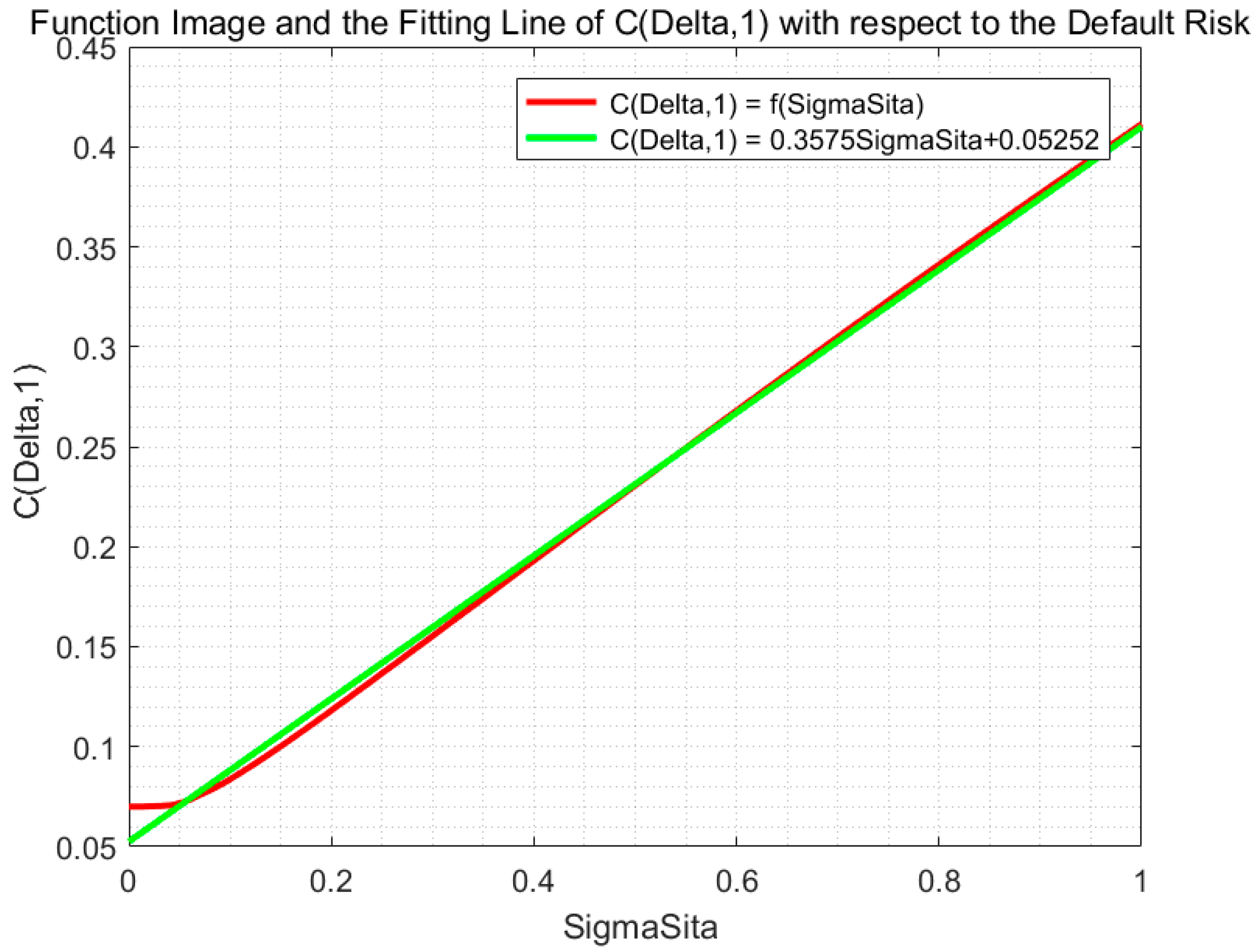
According to Equation (5), the relationship between the total compensation and the default risk is indirectly due to the presence of the call option function. To solve this problem, as is shown in Figure 2, we first drew the fitting map of the function image of call option with respect to the default risk, then, to get the specific function of the fitting line, we used the MATLAB software (Harbin Institute of Technology, Harbin, China).
The result is shown in Equation (53):
C ( Δ , 1 ) = 0.3575 σ θ + 0.05252
The statistic calculated by MATLAB is as follows: Goodness of fit: The sum of squares due to error ( S S E ) was 1.549 e 31 ; the coefficient of determination ( R S q u a r e ) was 1 ; the degree-of-freedom adjusted coefficient of determination ( A d j u s t e d   R S q u a r e ) was 1 ; and the root mean square error ( R M S E ) was 9.278 e 17 . As a consequence, Equation (53) is a very good fit for Equation (2), especially when σ θ > 0.05 , as is shown in Figure 2.
On the basis of Equations (5) and (53), we also have the following:
T C = ( 1 + μ ) [ λ ω E q ( 0 ) ( 0.3575 σ θ + 0.05252 ) + C S ]
σ θ = 1 0.3575 [ ( T C 1 + μ C S ) / λ ω E q ( 0 ) 0.05252 ]
λ = ( T C 1 + μ C S ) / ω E q ( 0 ) ( 0.3575 σ θ + 0.05252 )
In general, to be similar with Equations (53), (54), (55) and (56), we have the following:
C ( Δ , 1 ) = ρ 1 σ θ + ρ 2
T C = ( 1 + μ ) [ λ ω E q ( 0 ) ( ρ 1 σ θ + ρ 2 ) + C S ]
σ θ = 1 ρ 1 [ ( T C 1 + μ C S ) / λ ω E q ( 0 ) ρ 2 ]
λ = ( T C 1 + μ C S ) / ω E q ( 0 ) ( ρ 1 σ θ + ρ 2 )
where ρ 1 is the fit slope and ρ 2 is the fit intercept calculated by MATLAB.
Equations (58)–(60) are the fitting linear model of long-term compensation.

4.2. Simulation Analysis

4.2.1. Significance of Fitting Maps

Figure 3, Figure 4, Figure 5 and Figure 6 verify the conclusion in Section 3. Since the function in the long-term total compensation model contains an option function and the option function is a multivariate implicit function, it is impossible to directly write the expression between the risk and the option price, but it can be drawn using the specific point method and MATLAB software (Harbin Institute of Technology, Harbin, China) to obtain the fitting map related to T C . From the fitting map, we obtained other information not directly determined from the equations.
Overall, the data in Figure 3, Figure 4, Figure 5 and Figure 6 were calculated in Section 4.1. The specific data used in the figure of the function image and the basis of the propositions or corollaries in this paper are introduced in the note below each figure.

4.2.2. Analysis of Simulation Result

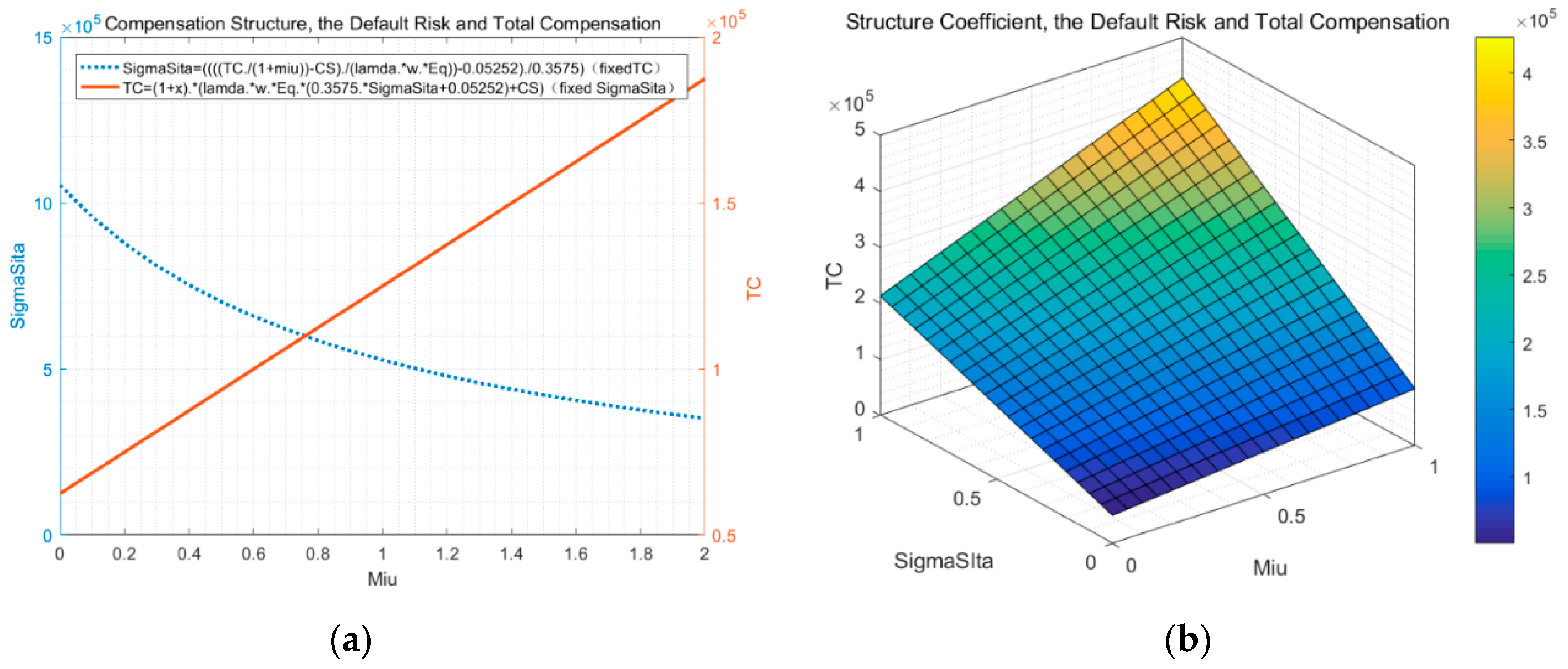
Figure 3a illustrates the total compensation value ( T C ) and the corresponding default risk ( σ θ ) with respect to the structure coefficient ( μ ) , based on Corollary 4, Equation (58), and Equation (59) for Wells Fargo and Co. The image of the total compensation with respect to the structure coefficient was obtained by fitting the μ value to the corresponding T C value when σ θ was fixed by Equation (58) (see Figure 3a, orange-red solid line), and the image of the default risk of total compensation with respect to the structure coefficient was directly drawn when T C was fixed by Equation (59) (see Figure 3a, blue dotted line).
Figure 3b illustrates the total compensation value ( T C ) and the corresponding default risk ( σ θ ) with respect to the structure coefficient ( μ ) , based on Corollary 4 and Equation (58) for the example bank. Similar to Figure 6a, the image of the total compensation was obtained by fitting the μ value to the corresponding T C value and σ θ value from Equation (58). The colored bar in the right side of Figure 3b demonstrates the value of total compensation ( T C ) .
As is shown in Figure 3a, when holding the total compensation unchanged, the structure coefficient is negatively associated with the default risk. As a consequence, to accomplish the object of minimizing the bank’s default risk, we should increase the value of μ , that is, increase the weight of inside debt in the total compensation. Similarly, when holding the default risk unchanged, the structure coefficient is positively associated with the total compensation. As a consequence, to accomplish the object of maximize the banker’s total compensation, we should increase the value of μ , that is, increase the weight of inside debt in the total compensation. In a word, increasing the weight of inside debt in the total compensation is not only helpful for the reduction of the bank’s default risk, but also the increase of the banker’s total compensation.
Figure 3b shows that the total compensation arrives at its maximum when increasing the structure coefficient and the default risk at the same time, and it arrives at its minimum when decreasing both of them. So, the increasing of total compensation in the post time is at price of the bank’s stability. As a result, the total compensation should be controlled properly to not stimulate the over-risking incentive of bankers.
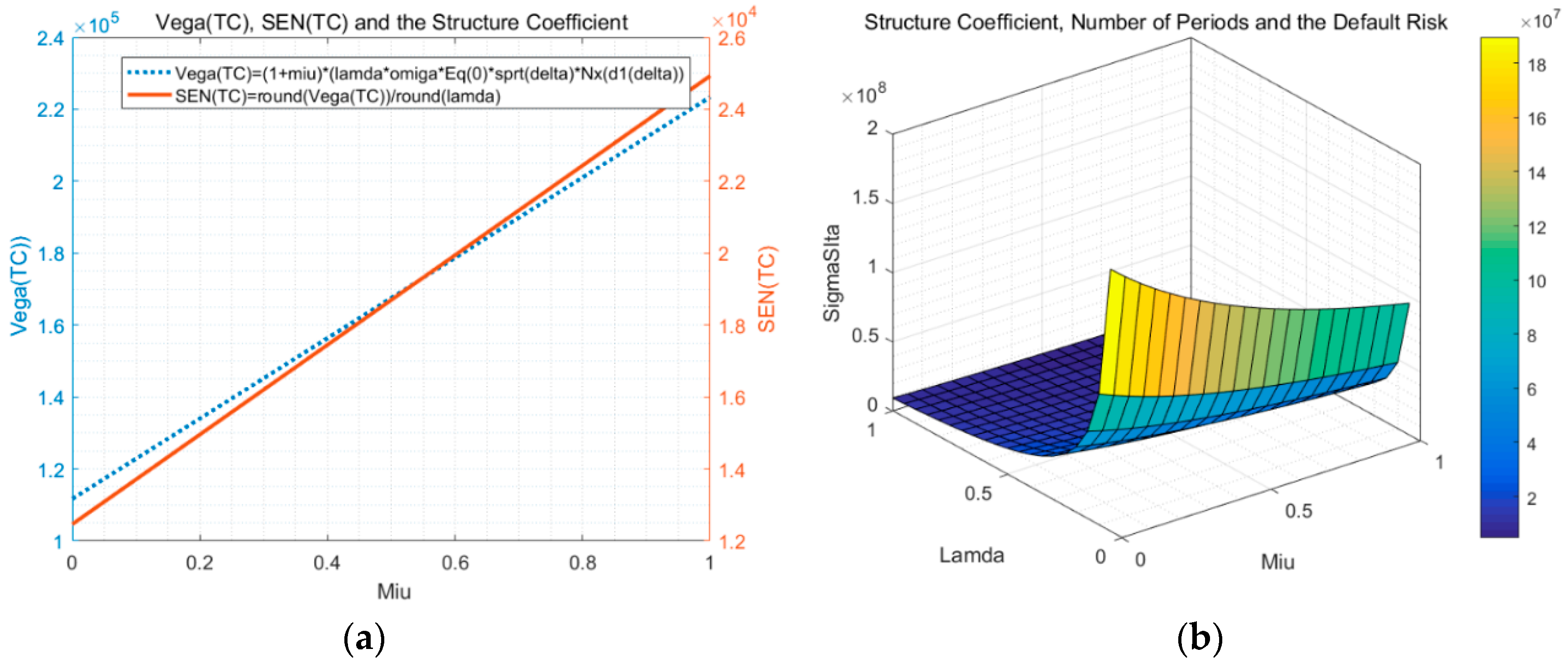
Figure 4a depicts the function image of the risk-taking incentive ( V e g a T C ) and the corresponding sensitivity of total compensation ( S E N T C ) with respect to the structure coefficient ( μ ) , based on Corollaries 2 and 3, Equations (6) and (7) for Wells Fargo and Co. As shown in the figure, the image of V e g a T C with respect to the structure coefficient ( μ )   was directly drawn when the default risk ( σ θ ) was fixed using Equation (6) (blue dotted line), and the image of S E N T C with respect to the structure coefficient ( μ ) was obtained when the default risk ( σ θ ) was fixed using Equation (7) (solid red line).
Figure 4b presents the three-dimensional image of the default risk ( σ θ ) and the corresponding number of periods ( λ ) with respect to the structure coefficient ( μ ) , based on Corollaries 4 and 5, and Equation (60) for Wells Fargo and Co. Similar to Figure 4a, the image of the default risk was obtained by fitting the μ value to the corresponding λ value and σ θ value obtained by Equation (60). The colored bar in the right side of Figure 4b demonstrates the value of the default risk ( σ θ ) .
As is shown in Figure 4a, when holding the default risk unchanged, the structure coefficient is positively associated with the risk-taking incentive. Similarly, when holding the default risk unchanged, the structure coefficient is positively associated with the sensitivity of total compensation. As a consequence, the structure coefficient exerts a positive impact on the risk-taking incentive and the sensitivity of total compensation when holding the default risk unchanged.
Figure 4b shows that the default risk arrives at its maximum when decreasing the structure coefficient and increasing the number of periods at the same time. As a result, decreasing the weight inside debt in the total compensation or increasing the number of periods is harmful for the reduction of the bank’s default risk.
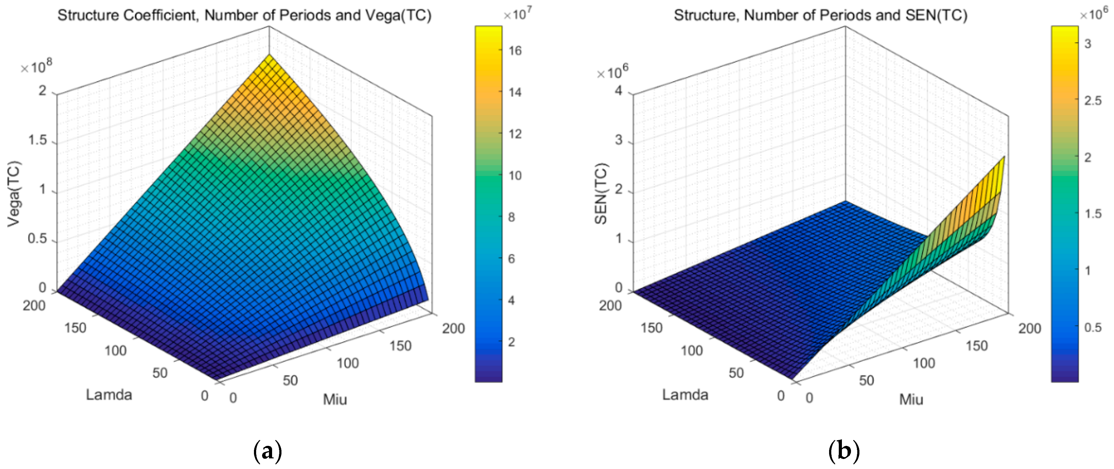
Figure 5a depicts the three-dimensional image of the risk-taking incentive ( V e g a T C ) and the corresponding structure coefficient ( μ ) with respect to the number of periods ( λ ) , based on Corollary 2, Corollary 5, and Equation (6) for Wells Fargo and Co. The image of the risk-taking incentive ( V e g a T C ) was obtained by fitting the μ value to the corresponding λ value and V e g a T C value when σ θ was fixed by Equation (6). The colored bar in the right side of Figure 5a demonstrates the value of the risk-taking incentive ( V e g a T C ) .
Figure 5b presents the three-dimensional image of the sensitivity of total compensation ( S E N T C ) and the corresponding the corresponding structure coefficient ( μ ) with respect to the number of periods ( λ ) , based on Corollaries 3 and 5, and Equation (7) for Wells Fargo and Co. Similar to Figure 5a, the image of the sensitivity of total compensation ( S E N T C ) was obtained by fitting the μ value to the corresponding λ value and S E N T C value when σ θ was fixed by Equation (7). The colored bar in the right side of Figure 5b demonstrates the value of the sensitivity of total compensation ( S E N T C ) .
As shown in Figure 5a, the risk-taking incentive of total compensation arrives at its maximum when increasing the structure coefficient and the number of periods at the same time, and it arrives at its minimum when decreasing both of them. As a result, the risk-taking incentives of total compensation produce a positive impact on the structure coefficient and the number of periods when holding the default risk unchanged.
Figure 5b shows that the sensitivity of total compensation arrives at its maximum when increasing the structure coefficient and the number of periods at the same time, and it arrives at its minimum when decreasing both of them. As a result, the sensitivity of total compensation has a positive impact on the structure coefficient and the number of periods when holding the default risk as unchanged.
Figure 6a shows the three-dimensional image of the risk-taking incentive ( V e g a T C ) and the corresponding default risk ( σ θ ) with respect to the structure coefficient ( μ ) , based on Corollary 2, Corollary 4, and Equation (6) for Wells Fargo and Co. The image of the risk-taking incentive ( V e g a T C ) was obtained by fitting the μ value to the corresponding σ θ value and V e g a T C value when λ was fixed by Equation (6). The colored bar in the right side of Figure 6a demonstrates the value of the risk-taking incentive ( V e g a T C ) .
Figure 6b presents the three-dimensional image of the sensitivity of total compensation ( S E N T C ) and the corresponding structure coefficient ( μ ) with respect to the number of periods ( λ ) , based on Corollary 3, Corollary 5, and Equation (7) for Wells Fargo and Co. Similar to Figure 6a, the image of the sensitivity of total compensation ( S E N T C ) was obtained by fitting the μ value to the corresponding σ θ value and S E N T C value when λ was fixed by Equation (7). The colored bar in the right side of Figure 6b demonstrates the value of the sensitivity of total compensation ( S E N T C ) .
Figure 6a shows that the risk-taking incentives of total compensation arrives at its maximum when increasing the structure coefficient and the default risk at the same time, and it arrives at its minimum when decreasing both of them. As a result, the risk-taking incentive of total compensation has a positive influence on the structure coefficient and default risk when holding the number of periods as unchanged.
A conclusion we drew from Figure 6b is that as the sensitivity of total compensation increases, the change of the default risk ( σ θ ) has a wavy style (positively, negatively, and positively associated) and the number of periods has a linear style (positively related) on the sensitivity of total compensation. To sum up, the sensitivity of total compensation arrives its maximum when increasing the structure coefficient and the default risk at the same time or when increasing the structure coefficient and decreasing the default risk at the same time.
To summarize: (a) Increasing the weight of inside debt in the total compensation is not only helpful for the reduction of the bank’s default risk, but also the increase of the banker’s total compensation; (b) the total compensation should be controlled properly to not stimulate the over-risking incentive of bankers; (c) the structure coefficient exerts a positive impact on the risk-taking incentive and the sensitivity of total compensation when holding the default risk as unchanged; (d) decreasing the weight of inside debt in the total compensation or increasing the number of periods is harmful for the reduction of bank default risk; (e) the risk-taking incentives of total compensation produce a positive impact on the structure coefficient and the number of periods when holding the default risk unchanged; (f) the sensitivity of the total compensation yield produces a positive impact on the structure coefficient and the number of periods when holding the default risk as unchanged; (g) the risk-taking incentive of total compensation has a positive influence on the structure coefficient and the default risk when holding the number of periods fixed; (h) the sensitivity of total compensation arrives at its maximum when increasing the structure coefficient and the default risk at the same time or when increasing the structure coefficient and decreasing the default risk at the same time.

4.3. Robustness

We used the data for Richard M. Adams Sr. of United Bankshares to perform the robustness test. He has been the chairman and CEO of United Bankshares since 1 January, 1984. His salary in 2006 was 641,667 USD. The results showed that our conclusion is robust and effective. The structure coefficient is negatively associated with the default risk when holding the total compensation unchanged, which is the same as the other conclusions. For instance, Δ = 10 10 = 1 :
C ( Δ , 1 ) = 0.3621 σ θ + 0.03771

5. Conclusions

In this study, we modeled a structure coefficient with respect to bank default risk, basing our findings on our previous work (Ma et al., 2020 [23]) regarding a banker’s long-term compensation, which has a linear relationship with a series of sequential call options on the bank’s return on equity, as determined by a practical calculation ( please see the summary of conclusions in this paper in Table A1, Appendix A). We demonstrated the relationship of the structure coefficient of total compensation with the bank’s default risk by formulating a particular formula. After setting the model of structure coefficient and default risk, we simulated the result using data from Wells Fargo and Co. to draw the function image in order to identify additional features. Firstly, we found an optimal situation about the structure coefficient for reducing a bank’s default risk, that is, that increasing the weight of inside debt in the total compensation is not only helpful for the reduction of a bank’s default risk, but also the increase of a banker’s total compensation. We are the first to calculate the expression of a structure coefficient which is irrelevant with other factors, except for the working time, current age, and tenure, and it is the simplest expression elucidated so far. At the same time, we are the first to find out the determinants of structure, that is, the working time, current age, and tenure. Last but not the least, we also have illustrated the influence of the number of periods. We expect our findings to offer help regarding the formulation of policies for pay contracts. This structure coefficient of a long-term total compensation model lays the foundation for further theoretical analysis, where, in prior studies, most researchers have only analyzed the compensation structure at a principle or statistic level, or from intuition, let alone via the determinants of it. Though limited theoretical analysis has been made, no specific model about the structure coefficient has been made which closes theoretical gap about the structure of pay contract in a way like us (using an expression which is irrelevant with risk). The economic explanation of this paper is that, from the perspective of corporate governance theory, executive compensation is one of the core factors to influence the risk-taking of the bank. Further, total compensation can be divided into three types, that is, inside equity, inside debt, and cash salary. We have found a way to express the proportion of inside debt in inside equity and cash salary and luckily this formula is irrelevant to ban risk. So, we can study the particular kinds of compensation related to bank risk and better design the pay contract of the banker. Besides, the practical significance is that the key of the following empirical analysis may focus on the indicators about compensation for the entire term, that is, the whole tenure of the banker, rather than an annual tenure. The shortcoming of our study is that, although the structure coefficient of compensation model has been theoretically expressed, due to the survival function, the calculating process is still complex and time-consuming. We will focus on the principle of executive decisions, which are the underlying cause of the uncertainty of the default risk, according to the precondition that the relationship between the default risk and the equity (net asset) of the bank is theoretically and statistically positive.

Author Contributions

Conceptualization, T.M. and M.J.; Methodology, T.M.; Software, T.M.; Validation, T.M., M.J., and X.Y.; Formal analysis, T.M.; Investigation, T.M.; Resources, T.M.; Data curation, T.M.; Writing—original draft preparation, T.M.; Writing—review and editing, T.M., M.J., and X.Y; Visualization, T.M.; Supervision, M.J.; Project administration, X.Y.; Funding acquisition, M.J. All authors have read and agreed to the published version of the manuscript.

Funding

This research was funded by the National Natural Science Foundation of China, grant number 71502044, and the China Postdoctoral Science Foundation, grant number 2015M570300.

Acknowledgments

We acknowledge Fu Zhenwu of Harbin Institute of Technology for their given help about the software MATLAB.

Conflicts of Interest

The authors declare no conflict of interest.

Appendix A

Table A1. Main conclusions of this paper.
ClassificationLong-Term Model Relationship   with   Compensation   Structure   ( μ )
From Predecessors or IntuitionFrom Theoretical AnalysisFrom Simulation ResultsCorresponding Figure
Total compensation ( T C ) Equation (5):
T C = ( 1 + μ ) ( λ ω E q ( 0 ) C ( Δ , 1 ) + C S )
Equation (58):
T C = ( 1 + μ ) [ λ ω E q ( 0 ) ( ρ 1 σ θ + ρ 2 ) + C S ]
( ? ) Corollary 1:
T C μ + 1 > T C μ
( + ) Figure 3a,b
Risk incentives of total compensation ( V e g a T C ) Equation (6):
V e g a T C = ( 1 + μ ) λ ω E q ( 0 ) e x p ( r Δ ) Δ N x ( d 2 ( Δ ) )
( ? ) Corollary 2:
V e g a T C ( μ + 1 ) > V e g a T C ( μ )
( + ) Figure 4a, Figure 5a and Figure 6a
Sensitivity of total compensation ( S E N T C ) Equation (7):
S E N T C = ( 1 + μ ) ω E q ( 0 ) 8 σ θ 2 ( 4 r 2 Δ + 4 σ θ 2 + 4 r Δ σ θ 2 + Δ σ θ 4 ) N x ( d 1 ( Δ ) )
( ? ) Corollary 3:
S E N T C ( μ + 1 ) > S E N T C ( μ )
( + ) Figure 4a, Figure 5b and Figure 6b
Bank default risk ( σ θ ) Equation (59):
σ θ = 1 ρ 1 [ ( T C 1 + μ C S ) / λ ω E q ( 0 ) ρ 2 ]
( ) Corollary 4:
μ σ θ < 0
( ) Figure 3a,b, Figure 4b and Figure 6a,b
Number of periods ( λ ) Equation (60):
λ = ( T C 1 + μ C S ) / ω E q ( 0 ) ( ρ 1 σ θ + ρ 2 )
( ? ) Corollary 5:
μ λ < 0
( ) Figure 4b and Figure 5a,b
Determinants of structureWorking time ( S ) ( + ) Corollary 6:
μ S + 1 > μ S
( + ) -
Current age ( A ) ( + ) Corollary 7:
μ A + 1 { > μ A , i f   A < 60 < μ A ,   i f   A > 60
( + ) and ( ) -
Tenure ( κ ) ( + ) Corollary 8:
μ κ + 1 < μ κ
( ) -
Compensation Structure ( μ ) Equation (9):
μ = M S κ n = m a x ( 0 , R A ) K A p ( n ) ( 1 + d ) n
Survival function ( p ^ ( n ) ) Lemma 1:
p ( n ) = { 1 ,   i f   n = 0 , 1 , 2 , , 65 A p ^ ( n ) ,   i f   n = 66 A , , 119 A 0 , i f   n = 120 A p ^ ( n ) = n + A = A + 1 n + A p ( S n + A )
Proposition 1:
μ = { 0.0175 S κ ( 1 1.0547 60 A + + 1 1.0547 65 A + p ( 66 A ) 1.0547 66 A + + p ( 119 A ) 1.0547 119 A ) , i f   A < 60 0.0175 S κ ( 1 1.0547 0 + + 1 1.0547 65 A + p ( 66 A ) 1.0547 66 A + + p ( 119 A ) 1.0547 119 A ) , i f   A > 60
Note: ( + ) stands for a positive relationship between the two variables, ( ) stands for a negative one, and ( ? ) stands for an unknown one.

References

  1. Jensen, M.C.; William, H.M. Theory of the firm: Managerial behavior, agency cost, and ownership structure. J. Financ. Econ. 1976, 3, 305–360. [Google Scholar] [CrossRef]
  2. Agnieszka, A.; Anna, S. Corporate Governance in the cooperative banking sector in Poland. Financ. Credit Act. Theor. Pract. 2019, 1, 4–15. [Google Scholar]
  3. Tang, C.H. Impacts of future compensation on the incentive effects of existing executive stock options. Int. Rev. Econ. Financ. 2016, 45, 273–285. [Google Scholar] [CrossRef]
  4. Shan, Y.; Walter, T. Towards a Set of Design Principles for Executive Compensation Contracts. Abacus 2016, 52, 619–684. [Google Scholar] [CrossRef]
  5. Kline, W. Executive compensation: An examination of the influence of TMT compensation on risk-adjusted performance. J. Strategy Manag. 2017, 10, 187–205. [Google Scholar] [CrossRef]
  6. Fried, J.M. Share Repurchases, Equity Issuances, and the Optimal Design of Executive Pay. Tex. Law Rev. 2011, 89, 1113–1147. [Google Scholar] [CrossRef] [Green Version]
  7. Dutcher, E.G. The Economic Psychology of Incentives: New Design Principles for Executive Pay. J. Econ. Psychol. 2018, 64, 140–142. [Google Scholar] [CrossRef]
  8. Conyon, M.J. Executive compensation and incentives. Acad. Manag. Perspect. 2006, 20, 25–44. [Google Scholar] [CrossRef]
  9. Canyon, M.J. Compensation Consultants and Executive Pay: Evidence from the United States and the United Kingdom. Acad. Manag. Perspect. 2009, 23, 43–55. [Google Scholar] [CrossRef]
  10. Burak, E. Is The Sky the Limit? Fair Executive Pay as Performance Rises. Soc. Probl. 2018, 65, 211–230. [Google Scholar] [CrossRef]
  11. Bebchuk, L.A. Managerial power and rent extraction in the design of executive compensation. Univ. Chic. Law Rev. 2002, 69, 751–846. [Google Scholar] [CrossRef]
  12. Banghoj, J. Determinants of executive compensation in privately held firms. Account. Financ. 2010, 50, 481–510. [Google Scholar] [CrossRef] [Green Version]
  13. Milidonis, A.; Nishikawa, T.; Shim, J. CEO Inside Debt and Risk Taking: Evidence from Property-Liability Insurance Firms. J. Risk Insur. 2019, 86, 451–477. [Google Scholar] [CrossRef]
  14. Deng, K.; He, J.; Kong, D.; Zhang, J. Does inside debt alleviate banks’ risk taking? Evidence from a quasi-natural experiment in the Chinese banking industry. Emerg. Mark. Rev. 2019, 40, 100622. [Google Scholar] [CrossRef]
  15. Chen, L.; Fan, H. CEO inside debt and bank loan syndicate structure. Rev. Financ. Econ. 2017, 34, 74–85. [Google Scholar] [CrossRef]
  16. Bhandari, A.; Mammadov, B.; Thevenot, M. The impact of executive inside debt on sell-side financial analyst forecast characteristics. Rev. Quant. Financ. Account. 2018, 51, 283–315. [Google Scholar] [CrossRef]
  17. Sheikh, S. CEO inside debt, market competition and corporate risk taking. Int. J. Manag. Financ. 2019, 15, 636–657. [Google Scholar] [CrossRef]
  18. Li, Z.F.; Lin, S.; Sun, S.; Tucker, A. Risk-adjusted inside debt. Glob. Financ. J. 2018, 35, 12–42. [Google Scholar] [CrossRef] [Green Version]
  19. Li, Y.; Zhang, X.-Y. Impact of board gender composition on corporate debt maturity structures. Eur. Financ. Manag. 2019, 25, 1286–1320. [Google Scholar] [CrossRef]
  20. Merton, R.C. On the Pricing of Corporate Debt: The Risk Structure of Interests Rates. J. Financ. 1974, 29, 449–470. [Google Scholar]
  21. Boyle, P.P.; Scott, W.R. Executive Stock Options and Concavity of the Option Price. J. Deriv. 2006, 13, 72–84. [Google Scholar] [CrossRef]
  22. Galletta, S.; Mazzù, S. Liquidity Risk Drivers and Bank Business Models. Risks 2019, 7, 89. [Google Scholar] [CrossRef] [Green Version]
  23. Pelizzon, L.; Subrahmanyam, M.G.; Tomio, D.; Uno, J. Sovereign credit risk, liquidity, and European Central Bank intervention: Deus ex machina? J. Financ. Econ. 2016, 122, 86–115. [Google Scholar] [CrossRef] [Green Version]
  24. Douglas, W. Diamond. Debt Maturity Structure and Liquidity Risk. Q. J. Econ. 1991, 106, 709–773. [Google Scholar]
  25. Imbierowicz, B.; Rauch, C. The Relationship between Liquidity Risk and Credit Risk in Banks. J. Bank. Financ. 2014, 40, 242–256. [Google Scholar] [CrossRef]
  26. Abad-Segura, E.; Cortés-García, F.J.; Belmonte-Ureña, L.J. The Sustainable Approach to Corporate Social Responsibility: A Global Analysis and Future Trends. Sustainability 2019, 11, 5382. [Google Scholar] [CrossRef] [Green Version]
  27. Ma, T. Pay Me Later is Not Always Positively Associated with Bank Risk Reduction—From the Perspective of Long-Term Compensation and Black Box Effect. Sustainability 2020, 12, 35. [Google Scholar] [CrossRef] [Green Version]
  28. Black, F.; Scholes, M. The Pricing of Options and Corporate Liabilities. J. Polit. Econ. 1973, 81, 637–654. [Google Scholar] [CrossRef] [Green Version]
  29. Kaplan, E.L.; Meier, P. Nonparametric estimation from incomplete observations. J. Am. Stat. Assoc. 1958, 53, 456–481. [Google Scholar] [CrossRef]
  30. The Period Life Table. Available online: http://www.ssa.gov/OACT/STATS/table4c6.html (accessed on 18 December 2019).
  31. Freund, S.; Latif, S.; Phan, H.V. Executive compensation and corporate financing policies: Evidence from CEO inside debt. J. Corp. Financ. 2018, 50, 484–504. [Google Scholar] [CrossRef]
  32. Hagendorff, J.; Vallascas, F. CEO pay incentives and risk taking: Evidence from bank acquisitions. J. Corp. Financ. 2011, 17, 1078–1095. [Google Scholar] [CrossRef]
  33. International Monetary Fund. Risk-taking by banks: The role of governance and executive pay. In Global Financial Stability Report: Risk-Taking, Liquidity, and Shadow Banking: Curbing Excess While Promoting Growth; IMF: Washington, DC, USA, 2014. [Google Scholar]
  34. Gopalan, R.; Milbourn, T.; Song, F.; Thakor, A.V. The Optimal Duration of Executive Compensation: Theory and Evidence AFA 2012 Chicago Meetings Paper. Available online: http://ssrn.com/abstract=1656603 (accessed on 10 November 2019).
  35. Sundaram, P.K.; Yermack, D.L. Pay me later: Inside debt and its role in managerial compensation. J. Financ. 2007, 62, 1551–1588. [Google Scholar] [CrossRef] [Green Version]
  36. Laeven, L.; Levine, R. Bank governance, regulation and risk taking. J. Financ. Econ. 2009, 93, 259–275. [Google Scholar] [CrossRef] [Green Version]
  37. Jokivuolle, E.; Keppo, J.; Yuan, X. Bonus Caps, Deferrals and Bankers’ Risk-Taking. Manag. Sci. under review.
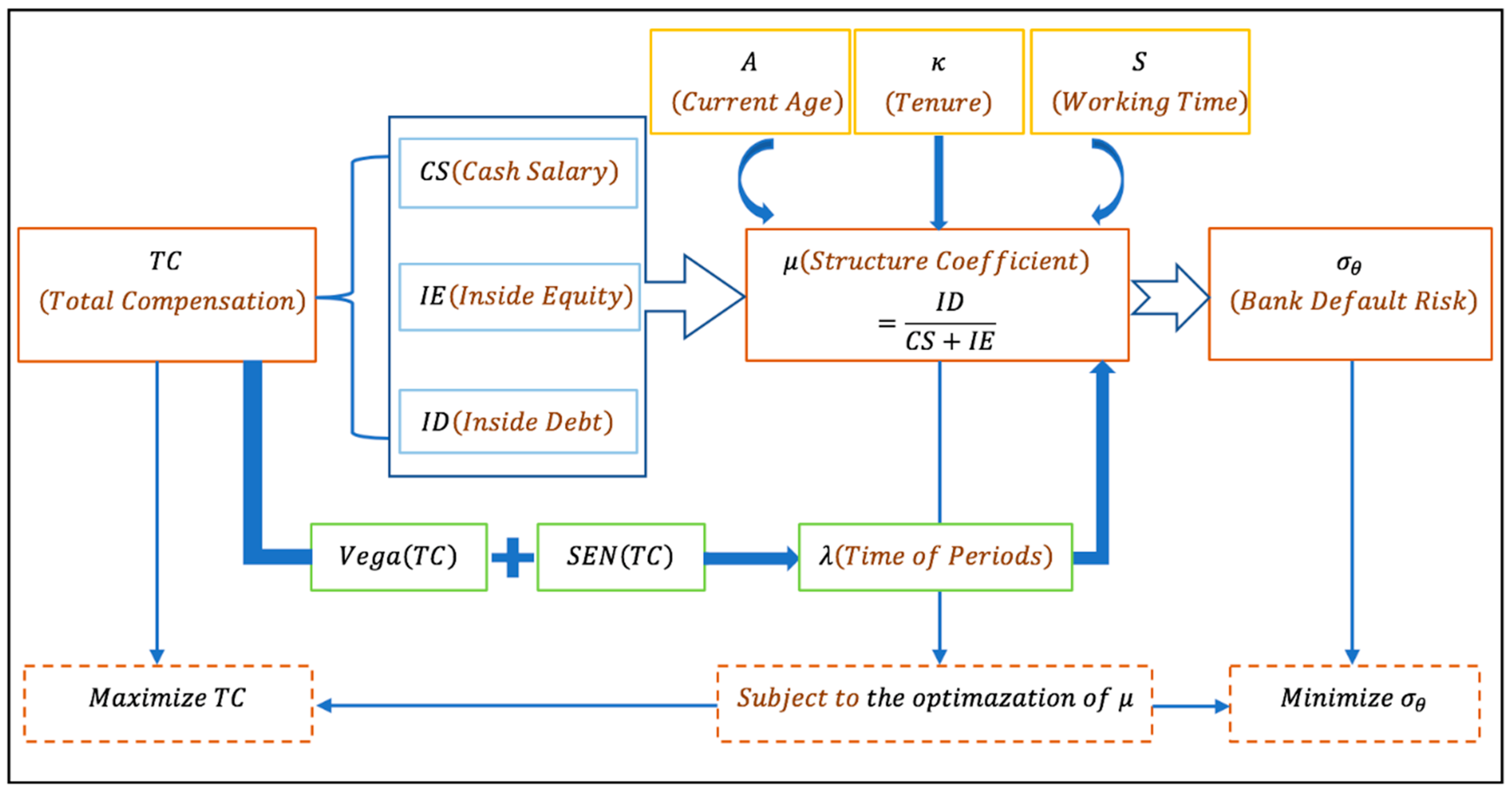
Figure 1. Schematic diagram of our research framework.
Sustainability 12 00666 g001
Figure 2. Function image and the fitting line of the call option ( C ( , 1 ) ) based on the BS model with respect to the default risk ( σ θ ) , based on Equations (2) and (53). Note: The red line is the true function image of the call option ( C ( , 1 ) ) based on BS model with respect to the default risk ( σ θ ) based on Equation (2), and the green one is the line in Equation (53), which was calculated by MATLAB.
Sustainability 12 00666 g002
Figure 3. (a) Function image of the total compensation value ( T C ) and the corresponding default risk ( σ θ ) with respect to the structure coefficient ( μ ) based on Corollary 4, Equation (58), and Equation (59). Note: Parameter values (for example, the bank being Wells Fargo and Co and the year of 2015): T C = 171 , 567 , 000 , 000 , E q ( 0 ) = 171567000 ,   ω = 0.000000295 ,   C S = 26538.88 , C ( , 1 ) = 0.3575 σ θ + 0.05252 ,   a n d   λ = 9 . The risk-free rate r is the mean of the one-month interest rate of national debt during November 2015 in the US. (b) Three-dimensional image of the total compensation value ( T C ) and the corresponding default risk ( σ θ ) with respect to the structure coefficient ( μ ) , based on Corollary 4 and Equation (58). Note: Parameter values (for example, the bank being Wells Fargo and Co and the year of 2015): E q ( 0 ) = 171 , 567 , 000 , 000 ,   ω = 0.000000295 ,   C S = 26538.88 , C ( , 1 ) = 0.3575 σ θ + 0.05252 ,   a n d   λ = 9 . The risk-free rate r is the mean of one-month interest rate of national debt during November 2015 in the US. The colored bar demonstrates the value of total compensation ( T C ) .
Sustainability 12 00666 g003
Figure 4. (a) Function image of the risk-taking incentive ( V e g a T C ) and the corresponding sensitivity of total compensation ( S E N T C ) with respect to the structure coefficient ( μ ) , based on Corollary 2, Corollary 3, Equation (6), and Equation (7). Note: Parameter values (for example, the bank being Wells Fargo and Co and the year of 2015): E q ( 0 ) = 171 , 567 , 000 , 000 ,   σ θ = 0.0737 ,   r = 0.07 , λ = 9 , μ = 0.7058 ,   κ = 9.326 ,   a n d   ω = 0.000000295 . The risk-free rate r is the mean of the one-month interest rate of national debt during November 2015 in the US. (b) Three-dimensional image of the default risk ( σ θ ) and the corresponding number of periods ( λ ) with respect to the structure coefficient ( μ ) , based on Corollaries 4 and 5, and Equation (60). (Note: Parameter values (for example, the bank being Wells Fargo and Co and the year of 2015): T C = 171567000 , E q ( 0 ) = 171 , 567 , 000 , 000 ,   ω = 0.000000295 ,   C S = 26538.88 , C ( , 1 ) = 0.3575 σ θ + 0.05252 ,   a n d   λ = 9 . The colored bar demonstrates the value of the default risk ( σ θ ) ).
Sustainability 12 00666 g004
Figure 5. (a) Three-dimensional image of the risk-taking incentive ( V e g a T C ) and the corresponding structure coefficient ( μ ) with respect to the number of periods ( λ ) , based on Corollary 2, Corollary 5, and Equation (6). Note: Parameter values (for example, the bank being Wells Fargo and Co and the year of 2015): E q ( 0 ) = 171 , 567 , 000 , 000 , , σ θ = 0.0737 ,   r = 0.07 ,   κ = 9.326 ,   a n d   ω = 0.000000295 . The risk-free rate r is the mean of the one-month interest rate of national debt during November 2015 in the US. The colored bar demonstrates the value of the risk-taking incentive ( V e g a T C ) . (b) Three-dimensional image of the sensitivity of total compensation ( S E N T C ) and the corresponding the corresponding structure coefficient ( μ ) with respect to the number of periods ( λ ) , based on Corollaries 3 and 5, and Equation (7). Note: Parameter values (for example, the bank being Wells Fargo and Co and the year of 2015): E q ( 0 ) = 171 , 567 , 000 , 000 ,   r = 0.07 ,   σ θ = 0.0737 , κ = 9.326 ,   a n d   ω = 0.000000295 . The risk-free rate r is the mean of the one-month interest rate of national debt during November 2015 in the US. The colored bar demonstrates the value of the sensitivity of total compensation ( S E N T C ) .
Sustainability 12 00666 g005
Figure 6. (a) Three-dimensional image of risk-taking incentive ( V e g a T C ) and the corresponding default risk ( σ θ ) with respect to the structure coefficient ( μ ) , based on Corollary 2, Corollary 4, and Equation (6). Note: Parameter values (for example, the bank being Wells Fargo and Co and the year of 2015): E q ( 0 ) = 171 , 567 , 000 , 000 , ,   r = 0.07 ,   λ = 9 , κ = 9.326 ,   a n d   ω = 0.000000295 . The risk-free rate r is the mean of the one-month interest rate of national debt during November 2015 in the US. The colored bar demonstrates the value of the risk-taking incentive ( V e g a T C ) . (b) Three-dimensional image of the sensitivity of total compensation ( S E N T C ) and the corresponding default risk ( σ θ ) with respect to the structure coefficient ( μ ) , based on Corollary 3, Corollary 4, and Equation (7). Note: Parameter values (for example, the bank being Wells Fargo and Co and the year of 2015): 171 , 567 , 000 , 000 ,   r = 0.07 ,   κ = 9.326 ,   ω = 0.000000295 ,   a n d   λ = 9 . The risk-free rate r is the mean of the one-month interest rate of national debt during November 2015 in the US. The colored bar demonstrates the sensitivity of total compensation ( S E N T C ) .
Sustainability 12 00666 g006
Table 1. Notation and definitions in our theoretical analysis.
ClassificationNotationDefinitionNotationDefinition
Compensation in long-term model T C Total compensation during banker’s tenure C S Cash salary during banker’s tenure
I E Inside equity during banker’s tenure I D Inside debt during banker’s tenure
λ The inside equity and inside debt frequency ω The fraction of equity
r The risk-free rate C ( ,   K C ) BS call option price
The time interval K C Strike price of the call option
N x ( x ) Standard cumulative normal distribution n x ( x ) Standard normal density
Structure coefficient μ Coefficient of compensation structure R The minimum retirement age
A Chief executive officer’s (CEO’s) current age κ / k a p p a The executive’s tenure
M A multiplier factor S The executive’s number of working years
d The firm’s cost of long-term debt K The terminal year of the pension
Survival function p ( n ) The probability that one is alive n years p ^ ( n ) Survival function in this paper
S a Survival probability D a Death probability
P j ^ Kaplan survival function n j The number under observations just after δ j Kaplan deaths
n j n j = n j + δ j δ j Death rate of Kaplan
Related measure V e g a T C Vega of total compensation S E N T C Sensitivity of total compensation
σ θ Volatility of return on equity (ROE)   E q ( i Δ ) The bank equity
ρ 1 Fit slope ρ 2 Fit intercept
Goodness of fit S S E Sum of squares due to error R S q u a r e Coefficient of determination
A j u s t e d   R S q u a r e Degree-of-freedom adjusted coefficient of determination R M S E Root mean square error
Note: When i Δ in the notation E q ( i Δ ) equals 0 , it ( E q ( 0 ) ) stands for the initial bank equity, i.e., the bank’s net asset value, BS call option price of C ( ,   K C ) is basing on Black and Scholes (1973) [28].
Table 2. The derivation process of the survival function p ^ ( n ) = a = A + 1 a p ( S a ) = n + A = A + 1 n + A p ( S n + A ) , i f   n = 66 A , , 119 A , A = 49 .
n Male   Exact   Age   a = n + A Death   Probability   p ( D a ) Survival   Probability   p ( S a ) = 1 p ( D a ) Survival   Function   p ^ ( n )   Value Formula   Derivation   p ^ ( n ) = a = A + 1 a p ( S a ) Value   of   p ( n ) n Male   Exact   Age   a = n + A Death   Probability   p ( D a ) Survival   Probability   p ( S a ) = 1 p ( D a ) Survival   Function   p ^ ( n )   Value Formula   Derivation   p ^ ( n ) = a = A + 1 a p ( S a ) Value   of   p ( n )
0490.0052080.9947921 1 136850.1124680.8875320.283633746 = a = 50 85 p ( S a ) 0.283633746
1500.0056570.9943430.994343 = a = 50 50 p ( S a ) 137860.1241640.8758360.248416646 = a = 50 86 p ( S a ) 0.248416646
2510.0061340.9938660.9882437 = a = 50 51 p ( S a ) 138870.1369170.8630830.214404184 = a = 50 87 p ( S a ) 0.214404184
3520.0065950.9934050.981726233 = a = 50 52 p ( S a ) 139880.1507540.8492460.182081896 = a = 50 88 p ( S a ) 0.182081896
4530.0070270.9929730.974827643 = a = 50 53 p ( S a ) 140890.1657040.8342960.151910197 = a = 50 89 p ( S a ) 0.151910197
5540.0074570.9925430.967558353 = a = 50 54 p ( S a ) 141900.1817890.8182110.124294594 = a = 50 90 p ( S a ) 0.124294594
6550.0079210.9920790.959894323 = a = 50 55 p ( S a ) 142910.1990190.8009810.099557608 = a = 50 91 p ( S a ) 0.099557608
7560.0084670.9915330.951766898 = a = 50 56 p ( S a ) 143920.2173960.7826040.077914183 = a = 50 92 p ( S a ) 0.077914183
8570.0091210.9908790.943085832 = a = 50 57 p ( S a ) 144930.2369060.7630940.059455845 = a = 50 93 p ( S a ) 0.059455845
9580.0099120.9900880.933737965 = a = 50 58 p ( S a ) 145940.2575250.7424750.044144479 = a = 50 94 p ( S a ) 0.044144479
10590.0108270.9891730.923628384 = a = 50 59 p ( S a ) 146950.2780310.7219690.031870945 = a = 50 95 p ( S a ) 0.031870945
11600.0118580.9881420.912675999 = a = 50 60 p ( S a ) 147960.2981110.7018890.022369866 = a = 50 96 p ( S a ) 0.022369866
12610.0129660.9870340.900842242 = a = 50 61 p ( S a ) 148970.3174320.6825680.015268955 = a = 50 97 p ( S a ) 0.015268955
13620.0141230.9858770.888119647 = a = 50 62 p ( S a ) 149980.3356550.6643450.010143854 = a = 50 98 p ( S a ) 0.010143854
14630.0153120.9846880.874520759 = a = 50 63 p ( S a ) 150990.3524380.6475620.006568774 = a = 50 99 p ( S a ) 0.006568774
15640.0165670.9834330.860032574 = a = 50 64 p ( S a ) 1511000.370060.6299400.004137934 = a = 50 100 p ( S a ) 0.004137934
16650.0179760.9820240.844572628 = a = 50 65 p ( S a ) 1521010.3885630.6114370.002530086 = a = 50 101 p ( S a ) 0.002530086
17660.0195640.9804360.828049409 = a = 50 66 p ( S a ) 0.828049409531020.4079910.5920090.001497834 = a = 50 102 p ( S a ) 0.001497834
18670.0212910.9787090.810419409 = a = 50 67 p ( S a ) 0.810419409541030.428390.5716100.000856177 = a = 50 103 p ( S a ) 0.000856177
19680.0231620.9768380.791648475 = a = 50 68 p ( S a ) 0.791648475551040.449810.5501900.00047106 = a = 50 104 p ( S a ) 0.00047106
20690.0252170.9747830.771685475 = a = 50 69 p ( S a ) 0.771685475561050.47230.5277000.000248578 = a = 50 105 p ( S a ) 0.000248578
21700.0275330.9724670.750438659 = a = 50 70 p ( S a ) 0.750438659571060.4959150.5040850.000125305 = a = 50 106 p ( S a ) 0.000125305
22710.0301310.9698690.727827192 = a = 50 71 p ( S a ) 0.727827192581070.5207110.4792896.00571 × 10−5 = a = 50 107 p ( S a ) 6.00571 × 10⁻⁵
23720.0329780.9670220.703824907 = a = 50 72 p ( S a ) 0.703824907591080.5467470.4532532.72211 × 10−5 = a = 50 108 p ( S a ) 2.72211 × 10⁻⁵
24730.0360860.9639140.678426681 = a = 50 73 p ( S a ) 0.678426681601090.5740840.4259161.15939 × 10−5 = a = 50 109 p ( S a ) 1.15939 × 10⁻⁵
25740.0395060.9604940.651624757 = a = 50 74 p ( S a ) 0.651624757611100.6027880.3972124.60523 × 10−6 = a = 50 110 p ( S a ) 4.60523 × 10⁻⁶
26750.0434150.9565850.623334468 = a = 50 75 p ( S a ) 0.623334468621110.6329280.3670721.69045 × 10−6 = a = 50 111 p ( S a ) 1.69045 × 10⁻⁶
27760.0477890.9522110.593545937 = a = 50 76 p ( S a ) 0.593545937631120.6645740.3354265.67021 × 10−7 = a = 50 112 p ( S a ) 5.67021 × 10⁻⁷
28770.0524640.9475360.562406143 = a = 50 77 p ( S a ) 0.562406143641130.6978030.3021971.71352 × 10−7 = a = 50 113 p ( S a ) 1.71352 × 10⁻⁷
29780.0574130.9425870.530116719 = a = 50 78 p ( S a ) 0.530116719651140.7326930.2673074.58036 × 10−8 = a = 50 114 p ( S a ) 4.58036 × 10⁻⁸
30790.0627890.9372110.49683122 = a = 50 79 p ( S a ) 0.49683122661150.7693270.2306731.05657 × 10−8 = a = 50 115 p ( S a ) 1.05657 × 10⁻⁸
31800.0688360.9311640.462631346 = a = 50 80 p ( S a ) 0.462631346671160.8077940.1922062.03078 × 10−9 = a = 50 116 p ( S a ) 2.03078 × 10⁻⁹
32810.0757240.9242760.42759905 = a = 50 81 p ( S a ) 0.42759905681170.8481830.1518173.08307 × −10 = a = 50 117 p ( S a ) 3.08307 × −10
33820.0834660.9165340.391909068 = a = 50 82 p ( S a ) 0.391909068691180.8905920.1094083.37313 × −11 = a = 50 118 p ( S a ) 3.37313 × −11
34830.0921440.9078560.355796999 = a = 50 83 p ( S a ) 0.355796999701190.9351220.0648782.18842 × −12 = a = 2 119 p ( S a ) 2.18842 × −12
35840.1018030.8981970.319575797 = a = 50 84 p ( S a ) 0.31957579771120----0
Note: See the period life table [30] at http://www.ssa.gov/OACT/STATS/table4c6.html. This table gives the probability of death within 1 year at each age between 0 and 119 for males and females. Death probability represents the probability of dying within one year. Number of lives stands for number of survivors out of 100,000 born alive. Note that the period life expectancy at a given age for 2004 represents the average number of years of life remaining if a group of persons at that age were to experience the mortality rates for 2004 over the course of their remaining life.
Table 3. John G. Stumpf’s compensation as CEO of Wells Fargo and Co ($).
Year Cash   Salary   Per   Year   ( C S y ) Inside   Debt   Value   Per   Year   ( I D y ) Inside   Equity   Value   Per   Year   ( I E y ) Total   Compensation   Value   Per   Year   ( T C y ) Return   on   Equity   ( R O E ) Total   Equity   Value   ( E q ( t ) )
2007749.61510,334.11011,083.720.244347,432,000,000
2008878.9210,061.95010,940.870.032470,949,000,000
2009560012,646.33028,491.730.1574105,846,000,000
20103239.84714,051.6610,245.40441,604.930.1486119,155,000,000
2011280015,979.9624,313.42251,497.130.167130,189,000,000
2012280019,538.0432,717.16864,298.740.1792145,953,000,000
2013280018,744.9341,960.70156,481.340.1908154,646,000,000
2014280020,853.0934,936.41658,523.760.1829166,075,000,000
2015280019,972.5834,870.67350,760.260.1735171,567,000,000
20162070.49822,660.327,987.68124,730.80.1602175,820,000,000
Sum C S = 26,538.88 I D = 164,842.9 I E = 207,031.465 T C = 398,413.3
Note: To simplify the calculation, we chose the value of 2015, which is shaded grey in the table.