Urbanization and the Urban–Rural Income Gap in China: A Continuous Wavelet Coherency Analysis

Abstract

This study applies wavelet analysis to examine the relationship between the urbanization and the urban–rural income gap in 31 provinces in China over the period 1978–2019. We find three patterns of causality between urbanization and the urban–rural income gap. Empirical results show that urbanization does Granger-cause an urban–rural income gap, the urban–rural income gap does Granger-cause urbanization, and there exists a two-way causality between the urban–rural income gap and urbanization. Furthermore, these relationships mainly exist at high frequencies (short term). The results obtained by considering the resident population are more significant than those by the registered population. These results could help local governments develop fair policies for urban and rural income distribution in the process of urbanization of different provinces, promoting the coordinated development between urban and rural areas.

1. Introduction

Urbanization has made a great contribution to China’s economic development in the past 40 years, and has also affected the relationship between urban and rural development. According to the data of China’s National Bureau of Statistics, China’s urbanization rate rose from 17.9 percent in 1978 to 60.6 percent at the end of 2019, and the ratio of per-capita disposable income of urban residents to that of rural residents increased from 2.5 in 1978 to 3.33 in 2009 and then decreased to 2.64 in 2019. Additionally, the ratio of per-capita consumption of urban residents to that of rural residents increased from 2.54 in 1978 to 3.35 in 2003 and then slowly decreased to 2.11 in 2019. This development gap causes an imbalance between urban and rural areas, which becomes the source of many social problems and has led scholars to focus on the relationship between urbanization and the urban–rural income gap.

Cities act as growth poles of regional economic development, which has both polarization and diffusion effects on the surrounding rural areas. In the early stages of urbanization (i.e., an urbanization degree less than 40%), cities primarily exert a polarization effect on their surrounding regions, and the urban–rural development gap tends to widen. In the middle stages of urbanization (i.e., an urbanization degree between 40 and 70%), the effect of cities on their surrounding regions gradually changes from polarization to diffusion, and the urban–rural development gap narrows. In the later stages of urbanization (i.e., an urbanization degree over 70%), there is gradual integration of urban and rural areas, and the urban–rural development gap starts to disappear [1]. Generally speaking, there exists an inverted U-shaped relationship between urbanization and urban–rural economic growth.

The contradiction between theoretical analysis and economic phenomena motivates us to explore whether the inverted U-shaped relationship between urbanization and urban–rural areas can be justified in China. The existing research papers do not have a definite conclusion because of their different research perspectives and methods. In addition, the level of development and urbanization is different in different regions in China. The relationship between urbanization and urban–rural income gap will change over time and region. The traditional measurement method can only grasp the relationship of linear invariance, but it is difficult to grasp the relationship with time and region change.

Given this view, we focus on the provincial level and examine the historical development and present characteristics of the relationship between urbanization and urban–rural development in various regions of China by a continuous wavelet coherency analysis. Wavelet analysis is one of the most efficient approaches for nonstationary time series data to explore time-frequency domain’s volatility. In addition to observing the phases of urbanization integration, our study uses wavelet coherence with a rolling window to evaluate the multihorizon nature of the changing comovement between urbanization and the urban–rural income gap in the short and long term.

2. Literature Review

Previous studies demonstrate that the relationship between urbanization and the urban–rural income gap is similar to a coin with two sides. One side regards the effect of urbanization on the urban–rural income gap, and the other side regards the effect of the urban–rural income gap on urbanization.

2.1. The Impact of Urbanization on the Urban–Rural Income Gap

Based on the literature, the effects of urbanization on the urban–rural income gap can be categorized into four types: negative, positive, variable according to certain factors, and uncertain.

Rauch studied the data for 1950, 1960, 1970, and 1980 from 17 Latin American countries and found urbanization narrows the urban–rural income gap [2]. Many scholars have carried out empirical research on China’s provincial data and found that urbanization has narrowed the gap between urban and rural development in China [3,4,5,6,7,8]. Therefore, Chinese scholars believe that accelerating urbanization is conducive to reducing the rural population, and reducing the urban–rural income gap by promoting the urbanization of population registration [9,10,11]. Why is there a coexistence of urbanization and a widening urban–rural income gap in China? To answer this, scholars have offered three explanations: reduced employment from industrial development, inadequate rural development and urban labor-market discrimination [12].

Migrant workers have become a common phenomenon in Chinese cities, and the decrease of the rural labor force will lead to the decline of rural residents’ income, which is conducive to widening the income gap between urban and rural areas [13,14]. Meanwhile, China’s urbanization strategy is partial to city development. Over the long term, the positive impact of urbanization on widening the urban–rural income gap becomes increasingly apparent [15]. Many empirical papers on China’s data have found that urbanization has widened the gap between urban and rural development [16,17,18].

In a departure from these straightforward research strategies, Chen adopted the Kuznets inverted-U hypothesis and argued that an inverted-U relationship exists between the urban–rural income gap and urbanization [19]. Some theoretical and empirical analysis proved that an inverted-U relationship also exists between urbanization and the urban–rural income gap in China [20,21,22]. Additionally, the effect of urbanization on the urban–rural income gap is regulated by several other factors. For example, the effect has obvious temporal and spatial disparities and varies by region depending on the degree of urbanization and the urban–rural income gap [23]. Ouyang found that there are three patterns of the relationships between urbanization and urban–rural development: widening, narrowing, or no impact. The relationship varies by economic development, urbanization level, agricultural labor resource and arable land resources [24]. The relationship between urbanization and the urban–rural income gap differs in central, western, eastern, and northern China [25]. In addition, the effect of urbanization on the urban–rural income gap was insignificant for many years. Only when the level of urbanization exceeds a threshold can it narrow the income gap between urban and rural areas [26]. There is also an income gap threshold for the effect of urbanization on the urban–rural income gap. When the urban–rural income ratio exceeds 2.54, urbanization widens the urban–rural income gap. In contrast, when the urban–rural income ratio falls below 2.54, urbanization effectively narrows the urban–rural income gap [27]. Urbanization widened the urban–rural income gap in the short term and narrowed the urban–rural income gap in the long term [28,29]. Meanwhile, some papers found an opposite conclusion. Urbanization has an immediate alleviating effect on income inequality, and also has a lagged aggravating effect on income inequality [30,31].

Other scholars have determined that urbanization has both positive and negative effects on reducing the urban–rural income gap in China [32,33]. This also makes the effect of urbanization on the urban–rural income gap to be nonsignificant [34,35].

2.2. The Impact of the Urban–Rural Income Gap on Urbanization

Current research on the effect of the urban–rural gap on urbanization is primarily focused on whether the income gap results in urbanization. Some classical theoretical and empirical analysis proved that urban–rural gap is a main driving force of urbanization in developed countries [36,37,38], such as the US and France [39,40]. In China, in addition to the economic factor of urban–rural income gap, government behavior is also the main factor affecting urbanization [41]. However, income disparity between urban and rural areas hinders labor migration, which, in turn, does harm to the urbanization process [42,43].

To summarize, scholars have been unable to reach a unified conclusion on the relationship between urbanization and the income gap. Views are particularly diverse among scholars who focus on China. This diversity could be a matter of research perspective and measurement method. After all, China is vast and has significant regional differences. In addition, during the urbanization process, the interaction of government and market forces means that spatial and temporal differences may occur in the relationship between urbanization and the urban–rural income gap. However, relying primarily on traditional econometric methods, such as the Granger causality test, Vector autoregression(VAR) model estimation, Structural vector autoregression (SVAR) model estimation, impulse response and variance decomposition, the co-integration test, Error correction model (ECM) estimation, and Vector error correction model(VECM) estimation, the cited studies had difficulty identifying those spatial and temporal differences. In terms of research content, the questions that the cited studies attempted to answer can be categorized into four types: (1) whether there is a correlation between the urban–rural income gap and urbanization; (2) the degree of correlation between the income gap and urbanization; (3) how this correlation evolves dynamically; and (4) whether there is a delay in the response of one factor due to a change in the other. Regrettably, no research has been able to systematically and comprehensively address all these questions simultaneously, and, to a large extent, the findings have been unable to accurately reflect the dynamic correlation between a country’s urbanization process and its urban–rural income gap.

Compared to the relatively traditional measurement methods employed by these domestic and foreign scholars, a current international trend is to employ wavelet coherency analysis, which is an advanced econometric method. Wavelet coherency analysis can not only effectively capture the structural changes between the time series in the time domain but also clearly differentiate the short-, medium-, and long-term relationships between the time series in the frequency domain. Therefore, compared to conventional measurement methods, wavelet coherency analysis can provide a comprehensive survey of both time and frequency problems between time series when examining urbanization and the urban–rural income gap. In addition, the vast majority of time series in economics are nonstationary, and wavelet coherency analysis is highly suitable for processing and analyzing nonstationary economic and financial time series.

This paper systematically and simultaneously examines the correlation between urbanization and the urban–rural income gap in China and the degree as well as dynamic evolution of this correlation over the short, medium, and long term. In this way, the paper provides a comprehensive review, analysis, and assessment of the relationship between urbanization and the urban–rural income gap in China over the last 40 years.

3. Methodology

In many previous studies, the analysis of a time series is exclusively done in the time domain, and the frequency domain is ignored. However, some appealing relations may exist at different frequencies. To stress such problems, a general practice is to utilize Fourier analysis to expose relations at different frequencies between variables of interest. However, the main shortcomings of the use of the Fourier transform for analysis has been argued to be the total loss of time information, thus making it difficult to discriminate ephemeral relations or to identify structural changes that are very important for time series macroeconomic variables for policy purposes. Another strong argument against the use of Fourier transform is the reliability of the results when the time series is nonstationary. As a solution to these aforementioned problems, wavelet transform offers a major advantage in terms of its ability to perform “natural local analysis of a time-series in the sense that the length of wavelets varies endogenously: it stretches into a long wavelet function to measure the low-frequency movements; and it compresses into a short wavelet function to measure the high-frequency movements” [44]. A wavelet possesses interesting features for conducting an analysis of a time series variable in a spectral framework but as function of time. In other words, wavelets show the evolution of change in the time series over time and at different periodic components, that is, frequency bands. In our work, we use continuous wavelet analysis tools, mainly wavelet coherence, to measure the degree of the local correlation between two time series in the time-frequency domain and the wavelet coherence phase differences.

3.1. Wavelet

A wavelet is a real-valued square integrable function, $\psi \in L^2(R)$ (A function x(t) is called a square integral if ${{\displaystyle {\int }_{-\infty }^{\infty }x(t)}}^2< \infty$) defined as:

$${\psi }_{u,s}(t)=\frac{1}{\sqrt{s}}\psi (\frac{t-u}{s}),$$

where the term $1/\sqrt{s}$ denotes a normalization factor ensuring unit variance of the wavelet, ${\Vert {\psi }_{u,s}\Vert }^2=1$. A wavelet has two control parameters, u and s. The location parameter u determines the exact position of the wavelet and the scale parameter s defines how the wavelet is stretched or dilated. Scale has an inverse relation to frequency; thus, a lower (higher) scale means a more (less) compressed wavelet that is able to detect higher (lower) time series frequencies. In addition, a wavelet needs to satisfy several conditions. The most important is the admissibility condition that ensures reconstruction of a time series from its wavelet transform. The admissibility condition is defined as:

$$C_{\psi }={\displaystyle {\int }_{-\infty }^{\infty }\frac{{\left|\psi (f)\right|}^2}{f}}df< \infty ,$$

where $\psi (f)$ is the Fourier transform of a wavelet $\psi (t)$. The admissibility condition implies that the wavelet does not have a zero frequency component; therefore, the wavelet has a zero mean, ${\displaystyle {\int }_{-\infty }^{\infty }\psi (t)}dt=0$. Further, the wavelet is usually normalized to have unit energy, that is, ${{\displaystyle {\int }_{-\infty }^{\infty }\psi (t)}}^{2}dt=1$, implying that the wavelet makes some excursion away from zero.

A large number of different wavelets exist. Each wavelet has its specific characteristics and is used for different purposes [45,46]. In our analysis, we use the Morlet wavelet, defined as:

$${\psi }^M(t)=\frac{1}{{\pi }^{1/4}}{e}^{i{\omega }_{0}t}{e}^{-t^2/2}.$$

Parameter ${\omega }_0$ denotes the central frequency of the wavelet. We set ${\omega }_0$ = 6, which is often used in economic applications [47,48]. The Morlet wavelet belongs to the family of complex or analytic wavelets; hence, this wavelet has both real and imaginary parts, allowing us to study both amplitude and phase.

3.2. The Continuous Wavelet Transform

The continuous wavelet transform $W_x(u,s)$ is obtained by projecting a specific wavelet $\psi (t)$ onto the examined time series $x(t)\in L^2(R)$:

$$W_x(u,s)={\displaystyle {\int }_{-\infty }^{\infty }x(t)}\frac{1}{\sqrt{s}}\psi (\frac{t-u}{s})dt.$$

An important feature of the continuous wavelet transform is the ability to decompose and then subsequently perfectly reconstruct a time series $x(t)\in L^2(R)$:

$$x(t)=\frac{1}{C_{\psi }}{\displaystyle {\int }_0^{\infty }\left[{\displaystyle {\int }_{-\infty }^{\infty }{W}_x(u,s){\psi }_{u,s}(t)du}\right]\frac{ds}{s^2},s}> 0.$$

Furthermore, the continuous wavelet transform preserves the energy of the examined time series:

$${\Vert x\Vert }^2=\frac{1}{C_{\psi }}{\displaystyle {\int }_0^{\infty }\left[{\displaystyle {\int }_{-\infty }^{\infty }{\left|W_x(u,s)\right|}^{2}du}\right]\frac{ds}{s^2}}.$$

We use this property for the definition of wavelet coherence, which measures the size of the local correlation between two time series.

3.3. Wavelet Coherence

To be able to study the interaction between two time series, we need to introduce a bivariate framework called wavelet coherence. For the proper definition of the wavelet coherence, we need to first introduce the cross wavelet transform and cross wavelet power. Torrence (1998) defined the cross wavelet transform of two time series x(t) and y(t) as:

$$W_{xy}(u,s)=W_x(u,s)W_y^{*}(u,s),$$

where $W_x(u,s)$ and $W_y(u,s)$ are continuous wavelet transforms of x(t) and y(t), respectively, u is a position index, s denotes the scale, and the symbol * denotes a complex conjugate. The cross wavelet power can be easily computed using the cross wavelet transform as $\left|W_{xy}(u,s)\right|$. The cross wavelet power reveals areas in the time-frequency space in which the time series shows a high common power; that is, it represents the local covariance between the time series at each scale.

The wavelet coherence can detect regions in the time-frequency space in which the examined time series comove but do not necessarily have a high common power. Following the approach of Torrence [49], we define the squared wavelet coherence coefficient as:

$$R^2(u,s)=\frac{{\left|S(s^{-1}{W}_{xy}(u,s))\right|}^2}{S(s^{-1}{\left|(W_x(u,s)\right|}^2)S(s^{-1}{\left|(W_y(u,s)\right|}^2)},$$

where S is a smoothing operator. The squared wavelet coherence coefficient is in the range $0\le R^2(u,s)\le 1$. Values close to zero indicate a weak correlation, whereas values close to one provide evidence of a strong correlation. Hence, the squared wavelet coherence measures the local linear correlation between two stationary time series at each scale and is analogous to the squared correlation coefficient in a linear regression.

Because the theoretical distribution for wavelet coherence is not known, we test the statistical significance using Monte Carlo methods. During the testing procedure, we follow the approach of Grinsted [50] and Torrence [51].

The use of wavelets brings with it the difficulty of dealing with boundary conditions on a dataset with a finite length. This problem is common to any transformation relying on filters. In our paper, we address this problem by padding the time series with a sufficient number of zeroes. The area, in which the errors caused by discontinuities in the wavelet transform cannot be ignored, where edge effects become important is called the cone of influence [50].

3.4. Phase Difference

To complete our analysis, we also use wavelet coherence phase differences to indicate details about the delays in the oscillation (cycles) between the two time series under study. we define the wavelet coherence phase difference as [49]:

$${\phi }_{xy}(u,s)={\tan }^{-1}\left(\frac{\mathcal{\Im }\left\{S\left(s^{-1}{W}_{xy}(u,s)\right)\right\}}{\mathcal{\Re }\left\{S\left(s^{-1}{W}_{xy}(u,s)\right)\right\}}\right),$$

where $\mathcal{\Im }$ and $\mathcal{\Re }$ are the imaginary and real parts, respectively, of the smooth power spectrum. The phase is indicated by arrows on the wavelet coherence plots. A zero phase difference means that the examined time series move together. The arrows point to the right (left) when the time series are in-phase (antiphase) or are positively (negatively) correlated. A phase difference of zero indicates that the time series move together at the specified frequency. If ${\phi }_{xy}\in (0,\frac{\pi }{2})$, then the series move in phase, but the time series y leads x. If ${\phi }_{xy}\in (-\frac{\pi }{2},0)$, then x is leading. A phase difference of π (or −π) indicates an antiphase relation. If ${\phi }_{xy}\in (\frac{\pi }{2},\pi )$, then x is leading. Time series y is leading if ${\phi }_{xy}\in (-\pi ,-\frac{\pi }{2})$.

4. Empirical Analysis

In consideration of the large differences in economic development between different provinces in China and the two different urbanization patterns of resident population and household registration in the urbanization process, we collected the following types of data for 1978 to 2019 for more than 31 regions in China: incomes of urban and rural residents, the urbanization rate calculated based on resident population, and the urbanization rate calculated based on household registration. The income and resident population data were drawn from the China Statistical Yearbook, while the household registration data were drawn from the China Public Health Statistical Yearbook.

Table 1. Descriptive statistics.

Stats	Urban_Live	Urban_Hukou	Incomegap
mean	0.375662	0.291519	2.556322
N	1110	1110	1104
p25	0.205694	0.164686	2.055642
p50	0.360688	0.242524	2.472794
p75	0.497427	0.378263	2.969523
max	0.896	0.903249	5.158974
min	0.076044	0.080657	0.974082
sd	0.190197	0.164692	0.716995
variance	0.036175	0.027123	0.514082
cv	0.506298	0.564944	0.280479

provides a brief overview of the statistical features of the data.

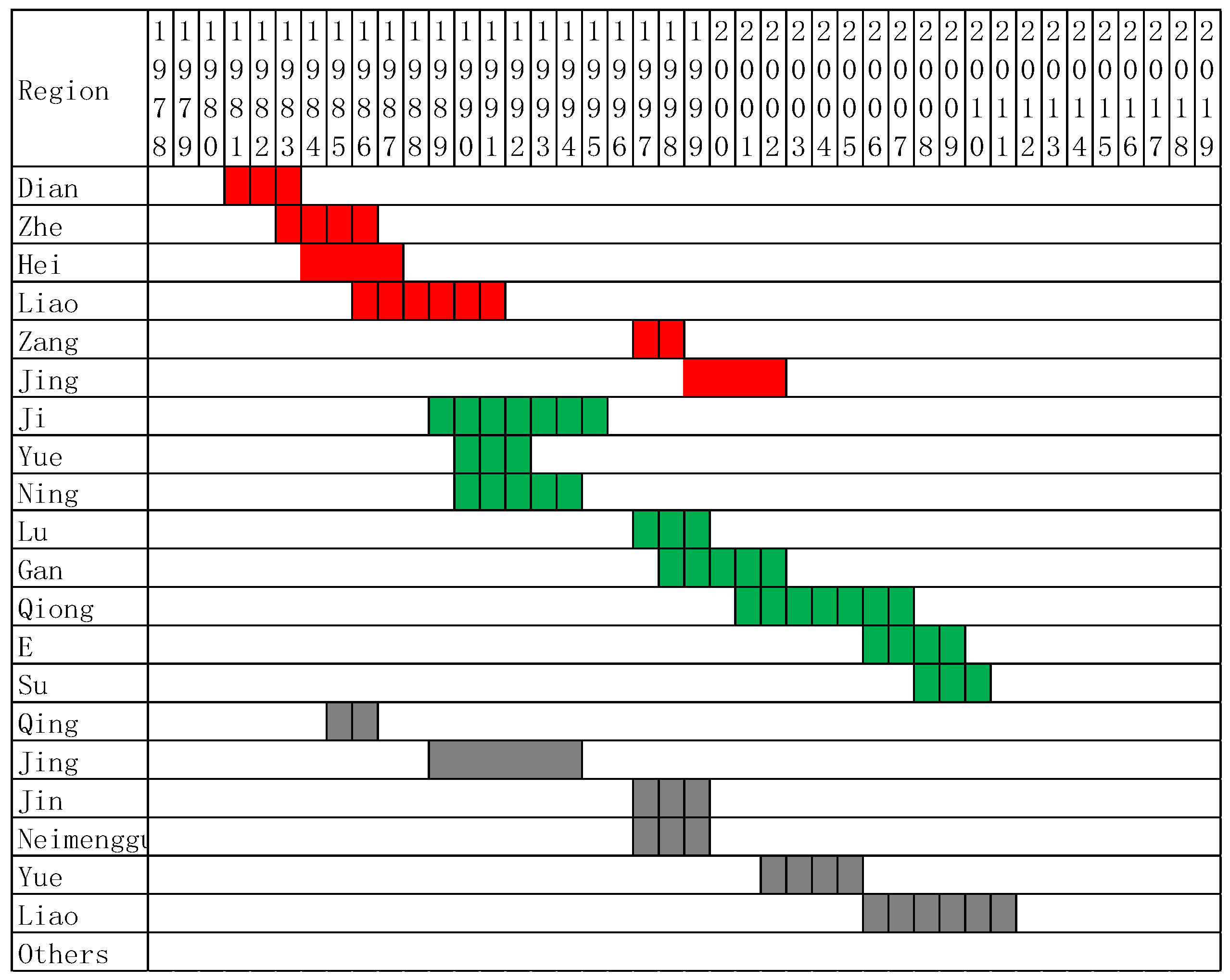
As the below result shows, we found three main types of relationship between urbanization and the urban–rural income gap. Figure 1 shows the results of analysis using the urbanization rate indicator of registered population. Figure 2 shows the results of analysis using the urbanization rate indicator of resident population. The first column is the abbreviation of provinces and cities. The red bar indicates that urbanization is positively related to the urban–rural income gap in the corresponding period of time, and urbanization leads to the urban–rural income gap. A green bar indicates that urbanization is positively related to urban–rural income gap, and the urban–rural income gap is ahead of urbanization, that is, the urban–rural income gap leads to urbanization. The bars are separated by vertical lines, indicating that the duration of causality is a short period of one to two years. Otherwise, it is a medium term of two to four years.

4.1. The Urban–Rural Income Gap Promotes Urbanization

The difference between agricultural and nonagricultural industries indicates the substantial differences in production efficiency between the urban and rural areas. While cities are a hub for nonagricultural industry, villages are the heart of agriculture. Not surprisingly, there is a substantial disparity in the incomes of the respective participants. Naturally, this disparity results in migration from villages to cities and is the primary expression of the differing role of production factors between urban and rural areas in the early stages of urbanization. Based on the data for 30 provinces or cities, this type of relationship could be observed at a historical point in 18 provinces or cities.

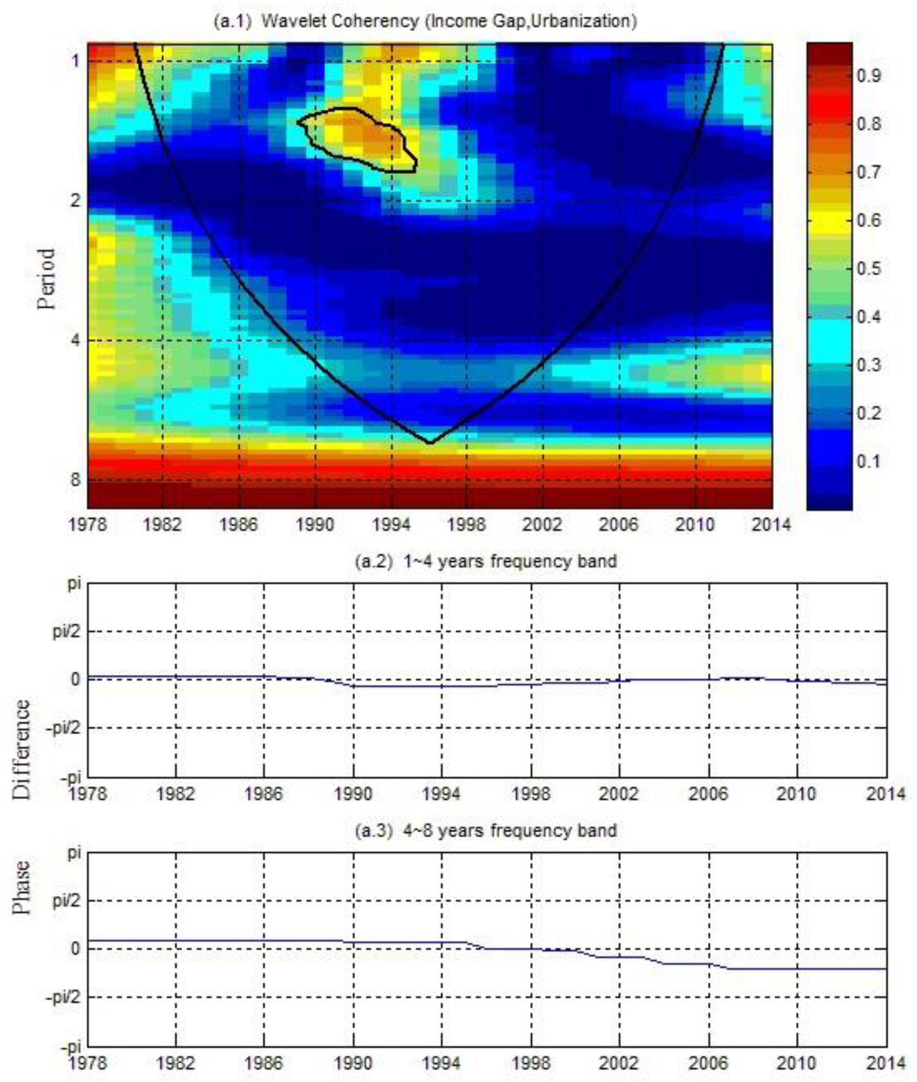
Using the wavelet coherency analysis outcome for Jilin as an example (Figure 3), we analyze the relationship between the urban–rural income gap and urbanization. In Diagram a.1, black lines are used to demarcate “islets” on the right. These “islets” indicate a significant relationship (at 5% levels of significance) between changes in the urban–rural income gap and changes in urbanization in certain parts of the time domain. The two symmetrical black curves enclose the cone of influence (COI). The area within the COI is one in which the correlation coefficient between the urbanization and the urban–rural income gap is susceptible to edge effects. The color-scale bar on the right indicates the correlation coefficient between the urbanization and the urban–rural income gap. Diagram (a.2) shows the phase difference between the urbanization and the urban–rural income gap in the one to four years frequency band, while Diagram (a.2) shows the phase difference between the urbanization and the urban–rural income gap in the four to eight years frequency band. For a more detailed interpretation of the relationship between changes in the urban–rural income gap and urbanization, this paper considers the one to two years frequency band to represent the short term, the two to four years frequency band to represent the medium term, and the four to eight years frequency band to represent the long term.

There is a highly positive correlation in the short term between the urbanization and urban–rural income gap in Jilin between 1989 and 1995, with a correlation coefficient greater than 0.7. In addition, changes in the urban–rural income gap precede changes in the urbanization. That is, urban–rural income standards resulted in additional urbanization [50,52].

4.2. Urbanization Widens the Urban–Rural Income Gap

As the growth poles of regional economic development, cities initially exert a polarization effect on surrounding rural areas. This polarization effect is followed by a diffusion effect. The polarization effect refers to cities attracting production factors from the rural areas. The urban economy benefits from agglomeration and urban production efficiency increases, thereby widening the urban–rural income gap. The diffusion effect occurs when the aggregation of such production factors surpasses a certain threshold and the urban economy no longer benefits from agglomeration. At this point, production factors diffuse from cities into the rural areas. This diffusion is accompanied by a transfer of technology to the rural areas, which narrows the urban–rural production efficiency gap and correspondingly the income gap. Chen and Xu argued that urbanization in China has reached the threshold at which the polarization effect is transforming into the diffusion effect. During the periods studied, urbanization seems to cause a significant narrowing of the urban–rural income gap [8]. However, this paper finds 13 provinces/cities in which urbanization results in an increase in the urban–rural income gap during certain time periods.

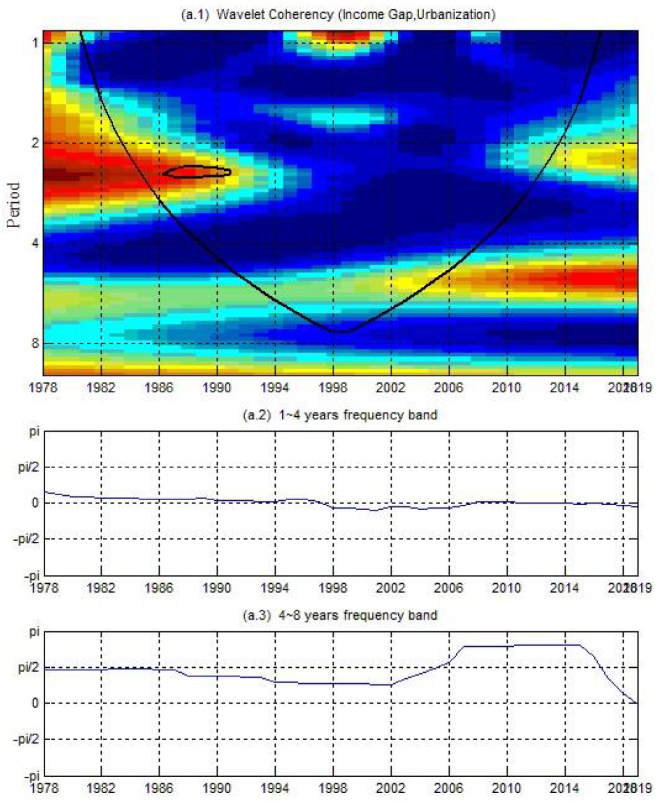
Using the analysis outcome for Heilongjiang, as an example (Figure 4.), we find a highly positive correlation in the medium term between the urbanization and the urban–rural income gap in Heilongjiang between 1986 and 1991, and urbanization precedes changes in the urban–rural income gap. That is, urbanization results in changes in the urban–rural income standards.

4.3. Reciprocal Causation between Urbanization and the Urban–Rural Income Gap

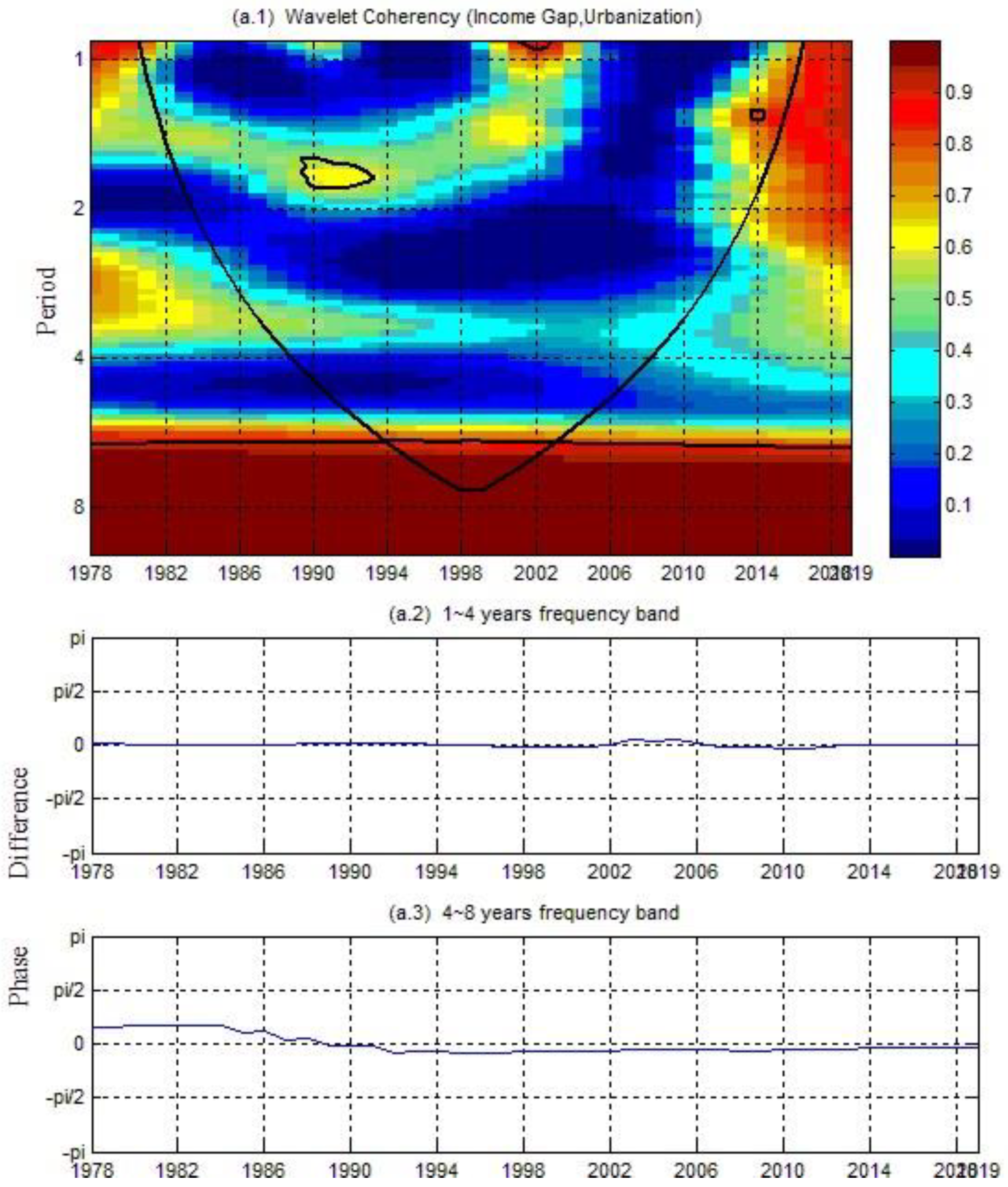
The relationship between urbanization and the urban–rural income gap involves more than one-way causality. In addition to appearing alternately in different cities and at different times, in certain cities and time periods, both relationships can appear simultaneously. This phenomenon is most evident in the analysis of Shanghai (Figure 5).It can be observed that between 1989 and 1993, a highly positive correlation appears between urbanization and the urban–rural income gap in Shanghai, with a correlation coefficient greater than 0.7. In addition, the phase difference fluctuates around 0 with small swing amplitudes. In fact, there seems to be a completely positive correlation, which attests to reciprocal causation. This correlation can also be observed in the following diagram, which was produced through an analysis of urbanization (calculated based on resident population) and the urban–rural income gap. It can also be observed in the analysis of urbanization (calculated based on household registration) and the urban–rural income gap, albeit slightly later (2004 to 2011).

To summarize, based on the time domain, in the last 40 years, the correlation between urbanization and the urban–rural income gap in China is high. More specifically, in the vast majority of the sampled provinces and cities, a significant positive correlation between urbanization and the urban–rural income gap is maintained most of the time. In particular, the conclusion that urbanization causes a widening of the urban–rural income gap is consistent with the views of most contemporary scholars [4,15,17,18,28]. Thus, cities continue to primarily exert a polarization effect on rural areas, which means that the current degree of urbanization has not reached the point that marks the start of a reversal. Coupled with the present economic policies in China, which continues to prioritize urban areas, it is not difficult to explain the widening urban–rural income gap that currently accompanies the urbanization process.

Based on the frequency domain, in the last 40 years, the relationship between urbanization and the urban–rural income gap in China is primarily a short-term relationship. A small number of provinces displayed a medium-term influence of two to four years, while only a few provinces exhibited a long-term influence of four to eight years: Inner Mongolia, Sichuan, Shanxi, Ningxia, and Qinghai. These findings are in stark contrast to those of Wang Zimin [15]. We believe that this difference in outcomes can be attributed to the numerous reforms in China that involve agriculture, farmer and rural area, townships enterprises, and urbanization during the last 40 years. The government actions undertaken in response to domestic economic fluctuations due to shocks in the global economy appear to be particularly significant. These actions have disrupted the medium- to long-term relationship between urbanization and the urban–rural income gap.

Last, a comparison was made between the results obtained for urbanization calculated using the registered households and urbanization calculated using the resident population. It was found that the relationship between urbanization and the urban–rural income gap was more pronounced and common when calculated using the resident population than when calculated using the registered households. In addition, the duration of the effect of urbanization on the urban–rural income gap calculated using the resident population was also longer. On the one hand, this outcome could be due to more stringent control by the government on household registration and a weaker relationship between the degrees of urbanization calculated based on registered households and economic development. On the other hand, this outcome could occur because the resident population is more aligned to the migratory characteristics of China’s highly mobile population. Thus, the urban–rural movement of population has a more significant impact on urban–rural economic development. Additionally, we found that differences between analysis outcomes regarding the degree of urbanization calculated using different methods tended to be more pronounced at the start of the studied period. This finding can be attributed to the government relaxing its grip on household registration and migrant workers settling down in the cities after time. This finding is also verified by the narrowing of the difference between the degree of urbanization calculated based on resident population and that calculated based on registered households after controls on household registration were relaxed.

5. Conclusions

Using continuous wavelet coherency analysis, this paper examined the relationship between urbanization and the urban–rural income gap in China from 1978 to 2014. The findings reveal a significant correlation between urbanization and the urban–rural income gap such that the urban–rural income gap is a significant cause of urbanization. In addition, urbanization contributes significantly to the urban–rural income gap in China. Our conclusions also indicate that the relationship between urbanization and the urban–rural income gap is primarily a short-term one with only a small number of provinces or cities experiencing medium- to long-term influence. We believe that this short-term effect is due to governmental action and China’s economic reform. Last, comparing the analysis outcome for urbanization based on resident population and with that based on registered households, we found the former to be more significant and common.

This paper provides a superior view of the relationship between urbanization and the urban–rural income gap in China at the provincial level since economic reform. It clearly differentiates the relationship between urbanization and the urban–rural income gap in different provinces and in different time frames, i.e., over the short, medium, and long terms. According to the above conclusion, we put forward the following three judgments on and suggestions for China’s urbanization. First, considering the positive effect of urbanization on economic growth and the limited harm to coordinated urban–rural development, urbanization will continue to advance. Since urbanization will only expand the gap between urban and rural development in the short and medium term, but not in the long run. China’s degree of urbanization lags behind that of other countries at similar levels of development. Second, the government should further improve the quality of urbanization and promote the people-oriented urbanization of the registered population, because the negative impact of urbanization of the registered population on urban–rural development relationship is less prominent than that of the permanent population. Third, in the process of continuing to promote urbanization, China should adjust measures to local conditions and adjust the level and speed of urbanization in combination with the actual situation of each province. At the same time, it should be supplemented by institutional arrangements to narrow the income gap between urban and rural areas, so as to promote urbanization scientifically and promote the coordinated development of urban and rural areas.

References

- Haodong, Q. The changing law of urban–rural relations in developed countries. Rural Econ. Soc. 1989, 2, 10–17. [Google Scholar]
- Rauch, J.E. Economic development, urban underemployment, and income inequality. Can. J. Econ. 1991, 26, 901–918. [Google Scholar] [CrossRef]
- Ming, L.; Zhao, C. Urbanization, urban-biased economic policies and urban–rural inequality. Econ. Res. J. 2004, 6, 50–58. [Google Scholar]
- Yaojun, Y. Financial development, urbanization and urban–rural income gap in China: Co-integration analysis and Granger causality test. China Rural Surv. 2005, 2, 2–8. [Google Scholar]
- Yu, C.; Xiaohong, C.; Yueru, M. Urbanization, the urban–rural income gap, and economic growth: An empirical study based on China’s provincial level panel data. Stat. Res. 2010, 3, 29–36. [Google Scholar]
- Qilin, M. Economic opening, urbanization and urban- rural income gap. Zhejiang Soc. Sci. 2011, 1, 11–23. [Google Scholar]
- Huang, S.X. Urban–rural income gap and urbanization development. Acad. Forum. 2009, 8, 136–139. [Google Scholar]
- Yiguo, C.; Jun, X. How urbanization affects balanced growth in urban–rural area in china. Econ. Theory Bus. Manag. 2016, 3, 72–85. [Google Scholar]
- Xue-chuan, S. Urbanization and income difference between urban and rural area. J. Cent. Univ. Financ. Economics. 2002, 3, 1–10. [Google Scholar]
- Lv, W.; Gao, F. Urbanization, citizenization and urban–rural income gap: Comparison and selection of citizenization measures under “double dual structure”. Financ. Trade Econ. 2013, 12, 38–46, 93. [Google Scholar]
- Li, G.Z.; Ai, X.Q. Measurement, evolution trend and influencing factors of income and consumption in urban and rural areas under “sharing” view. China Soft Sci. 2017, 11, 173–183. [Google Scholar]
- Fang, C. Why labor flow did not narrow the urban–rural income gap. Ind. Econ. Rev. 2006, 6, 4–10. [Google Scholar]
- Xiao, R. Urbanization, real estate prices and income gap between urban and rural areas: Base on provincial panel data analysis. Financ. Econ. 2013, 9, 100–107. [Google Scholar]
- Yuandong, G.; Na, Z. An analysis of the threshold effect of human capital on the reduction of urban–rural income gap in the process of urbanization in China. Inq. Econ. Issues 2018, 9, 42–51. [Google Scholar]
- Zimin, W. A reexamination of urbanization and urban–rural gap in China—from spatial panel perspective. Econ. Geogr. 2011, 8, 56–62. [Google Scholar]
- Hu, D.P. Trade, rural-urban migration, and regional income disparity in developing countries: A spatial general equilibrium model inspired by the case of China. Reg. Sci. Urban Econ. 2002, 32, 311–338. [Google Scholar] [CrossRef]
- Kaiming, C.; Jinchang, L. The mechanism behind and dynamic analysis of urban bias, urbanization and the urban–rural income gap. J. Quant. Tech. Econ. 2007, 24, 116–125. [Google Scholar]
- Xiaoyi, C. Urbanization, industrialization and the urban–rural income gap: A study based on the SVAR model. Econ. Surv. 2010, 6, 24–27. [Google Scholar]
- Zongsheng, C. Ladder-style variation of the inverted-U curve. Econ. Res. J. 1994, 5, 55–59. [Google Scholar]
- Yunbo, Z. Urbanization, urban–rural income gap and overall income inequality in China: An empirical test of the inverse-U hypothesis. China Econ. Q. 2009, 8, 1239–1256. [Google Scholar]
- Fenfen, Y.S.; Xu, W. The inverted u-shaped curve between Chinese urban–rural income inequality and urbanization rate. Manag. Rev. 2015, 27, 3–10. [Google Scholar]
- Yu-xiang, Y.; Pu-yun, W. The income distribution effect of china’s urbanization -theoretical and empirical evidence. Economist 2019, 9, 5–14. [Google Scholar]
- Fang, X. Spatial-temporal evolution of urbanization and urban–rural income disparity. Shanghai Econ. Review. 2015, 10, 114–120. [Google Scholar]
- Jinqiong, O.; Xiaoling, Z.; Yapeng, W. Spatial and temporal differences of urban and rural income gap influenced by urbanization. Stat. Decision. 2015, 4, 108–111. [Google Scholar]
- Su, C.W.; Liu, T.Y.; Chang, H.L. Is urbanization narrowing the urban–rural income gap? A cross-regional study of China. Habitat Int. 2015, 48, 79–86. [Google Scholar] [CrossRef]
- Zhou, S.F.; Qi, S.W.; Lu, Z.B. Region difference, urbanization and urban–rural income gap. China Popul. Resour. Environ. 2010, 20, 115–120. [Google Scholar]
- Junhua, G. The threshold effect of urbanization in China on the urban–rural income gap: An empirical study based on provincial-level panel data from China. Shanxi Caijing Daxue Xuebao 2009, 11, 23–29. [Google Scholar]
- Jing, L. An empirical analysis of the impact of urbanization on the urban–rural income gap. Co-Oper. Econ. Sci. 2007, 2, 67–74. [Google Scholar]
- Xian-hua, W. Relationship among urbanization, citizenization and urban–rural income inequality: An empirical analysis based on time series data and panel data of Shandong province. Geogr. Sci. 2011, 1, 68–73. [Google Scholar]
- Chen, G.; Glasmeier, A.K.; Zhang, M.; Shao, Y. Urbanization and income inequality in post-reform China: A causal analysis based on time series data. PLoS ONE 2016, 11, e0158826. [Google Scholar] [CrossRef]
- Xiaobo, Y.; Qiao, W. The study on financial development, urbanization and urban & rural residents’ income gap in china. Econ. Geogr. 2020, 3, 84–91. [Google Scholar]
- Zhiguo, D.; Xuankai, Z.; Jing, Z. Direct impact and the spatial spillover effect: The impact of urbanization on the urban–rural income gap. J. Quant. Tech. Econ. 2011, 9, 53–62. [Google Scholar]
- Changliang, L. Has urbanization narrowed the urban–rural income gap?: An empirical analysis based on panel data between 2004 and 2013 from 31 provinces nationwide. Res. Dev. 2015, 6, 132–145. [Google Scholar]
- Yifu, L.; Mingxing, L. Development strategy and industrialization of China. Econ. Res. J. 2004, 7, 48–58. [Google Scholar]
- Xiaoqi, L.; Xiaoping, K. Analysis of the correlation between urban and rural income gap, economic growth, industrialization and urbanization. Jiangxi Soc. Sci. 2011, 7, 20–32. [Google Scholar]
- Todaro, M.P. A model for labor migration and urban unemployment in less developed countries. Am. Econ. Rev. 1969, 59, 138–148. [Google Scholar]
- Gallaway, L.E.; Vedder, R.K. Mobility of Native Americans. J. Econ. Hist. 1971, 31, 613–649. [Google Scholar] [CrossRef]
- Tiebout, B.C. A pure theory of local expenditures. J. Political Econ. 2010, 64, 416–424. [Google Scholar] [CrossRef]
- Oates, W.E. The effects of property taxes and local public spending on property values: An empirical study of tax capitalization and Tiebout Hypothesis. J. Political Econ. 1969, 77, 957–971. [Google Scholar] [CrossRef]
- Binet, M.E. Testing for fiscal competition among French municipalities: Granger causality evidence in a dynamic panel data model. Pap. Reg. Sci. 2003, 2, 277–289. [Google Scholar] [CrossRef]
- Wenlin, F. Structural barriers to population movements: An analysis based on experience in public expenditure competition. J. World Econ. 2007, 30, 32–40. [Google Scholar]
- Chaoming, W.; Wenwu, M. Relations of balanced development of urban–rural education and urban–rural income gap with the new urbanization. Financ. Econ. 2014, 8, 97–108. [Google Scholar]
- Jiuwen, S.; Yulong, Z. Urban–rural disparity, labor migration and urbanization. Econ. Rev. 2015, 2, 29–40, 77. [Google Scholar]
- Aguiar-Conraria, L.; Soares, M.J. Business Cycle Synchronization and the Euro: A Wavelet Analysis. J. Macroecon. 2011, 33, 477–489. [Google Scholar] [CrossRef]
- Adisson, P. The Illustrated Wavelet Transform Handbook; The Institute of Physics: London, UK, 2002. [Google Scholar]
- Percival, D.B.; Walden, A.T. Wavelet Methods for Time Series Analysis; Cambridge University Press: New York, NY, USA, 2000; Volume 4. [Google Scholar]
- Aguiar-Conraria, L.; Azevedo, N.; Soares, M.J. Using wavelets to decompose the time-frequency effects of monetary policy. Phys. A Stat. Mech. Appl. 2008, 387, 2863–2878. [Google Scholar] [CrossRef]
- António, R. Money growth and inflation in the euro area: A time-frequency view. Oxf. Bull. Econ. Stats 2012, 74, 875–885. [Google Scholar]
- Torrence, C.; Webster, P.J. Interdecadal Changes in the ENSO-monsoon System. J. Clim. 1999, 12, 2679–2690. [Google Scholar] [CrossRef]
- Grinsted, A.; Moore, J.C.; Jevrejeva, S. Application of the cross wavelet transform and wavelet coherence to geophysical time series. Nonlinear Process. Geophys. 2004, 11, 561–566. [Google Scholar] [CrossRef]
- Torrence, C.; Compo, G. A practical Guide to Wavelet Analysis. Bull. Am. Meteorol. Soc. 1998, 79, 61–78. [Google Scholar] [CrossRef]
- Tiwari, A.K.; Mutascu, M.; Andries, A.M. Decomposing time-frequency relationship between producer price and consumer price indices in Romania through wavelet analysis. Econ. Modeling 2013, 31, 151–159. [Google Scholar] [CrossRef]
© 2020 by the authors. Licensee MDPI, Basel, Switzerland. This article is an open access article distributed under the terms and conditions of the Creative Commons Attribution (CC BY) license (http://creativecommons.org/licenses/by/4.0/).