Constructing an Environmental Friendly Low-Carbon-Emission Intelligent Transportation System Based on Big Data and Machine Learning Methods


Abstract
1. Introduction
2. Related Works
3. Motivation
4. Vehicle Emission Model
4.1. Acceleration or Deceleration
4.2. Cruising
4.3. Idling
5. Traffic Flow Prediction Method
- Accuracy: Accuracy is the most basic requirement. Accurate prediction of future traffic conditions is the basis for accurate navigation.
- Real-time: Real-time is the precondition of the application. The process of training, solving, and prediction of the model needs to have high efficiency. As the traffic flow varies greatly in a short time, once the predicted result loses its timeliness, it loses its significance.
- Adaptability: Adaptability is essential to guarantee the stability of the whole system. The traffic flow will be disturbed by many factors in a short time. The prediction model needs to be able to change flexibly and deal with different conditions through simple adjustment of parameters to ensure the stability of the system.
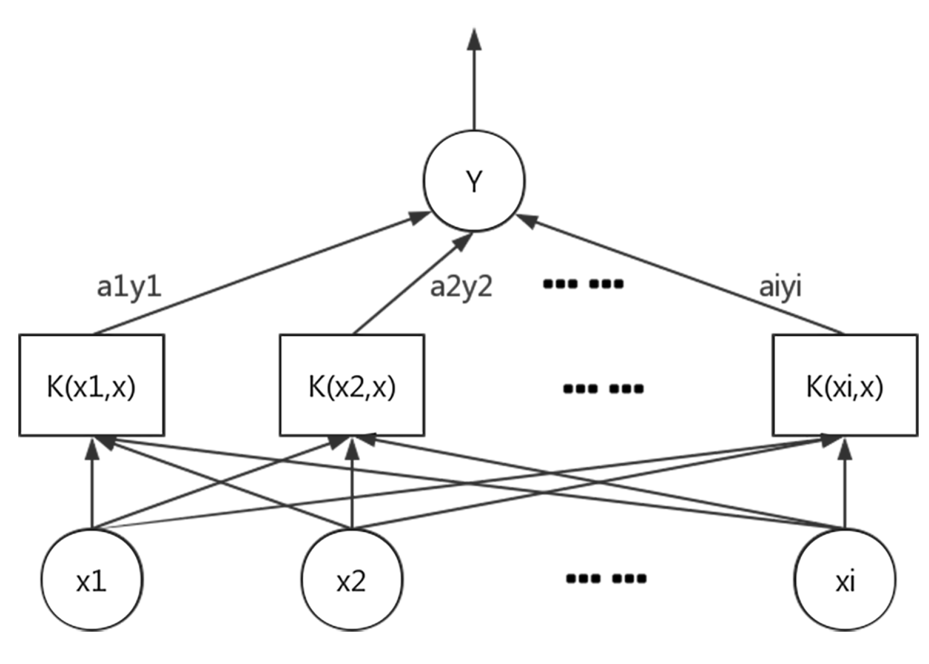
5.1. Traffic Flow Prediction Based on Support Vector Regression
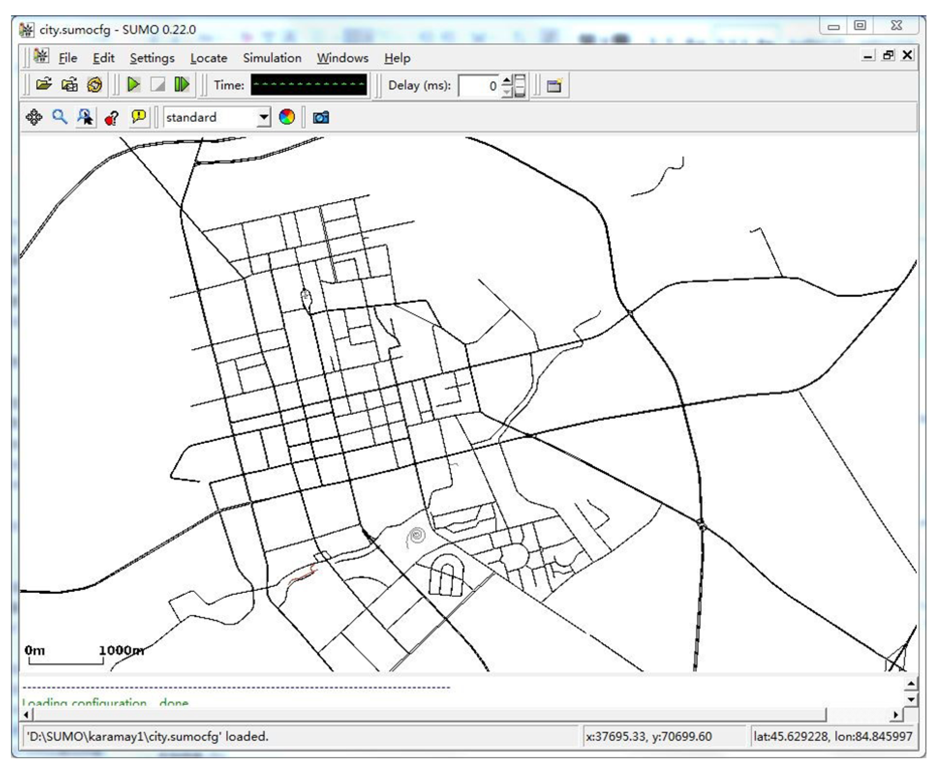
- Data Preparation: Extract historical data from the database. Construct a road map, calibrate coordinates, and transform historical data into traffic flow data. Normalize the data and divide them into a training set and a test set.
- Data Analysis: Analyze the characteristics of the data, choose parameters of SVR, and obtain the decision function.
- Model Construction: Build the SVR model with the training set. Evaluate the forecasting results using the test set. Finally, apply the model to real-time traffic flow data for real-time forecasting.
- Penalty coefficient C: It adjusts the proportion between empirical risk and expected risk so as to make the model get the best generalization ability.
- Insensitivity coefficient : It affects the number of support vectors, thus affecting the generalization ability of the model.
- Kernel function parameters : It influences the distribution of input samples in the feature space and the correlation between support vectors.
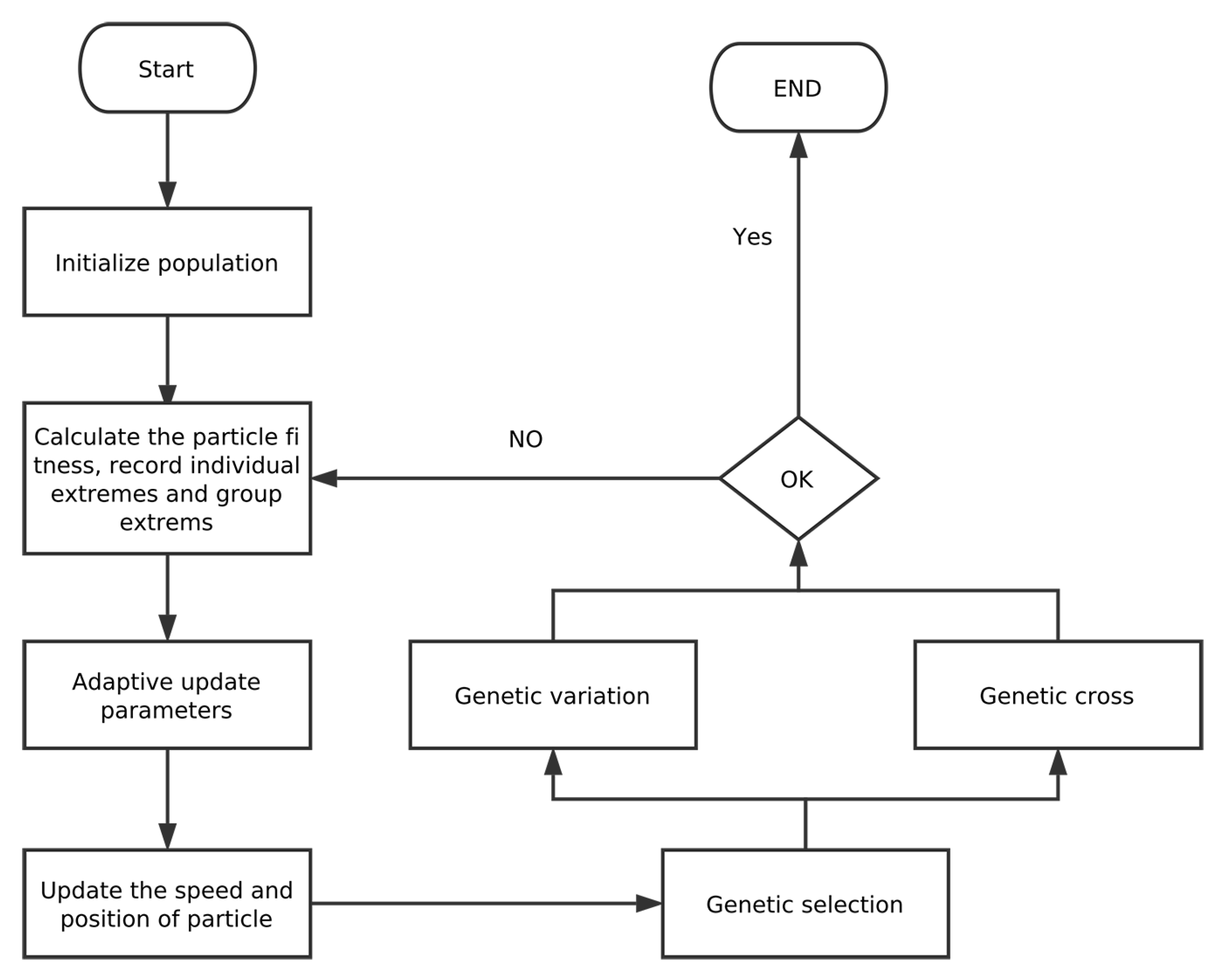
5.2. GAPSO-Enhanced SVR
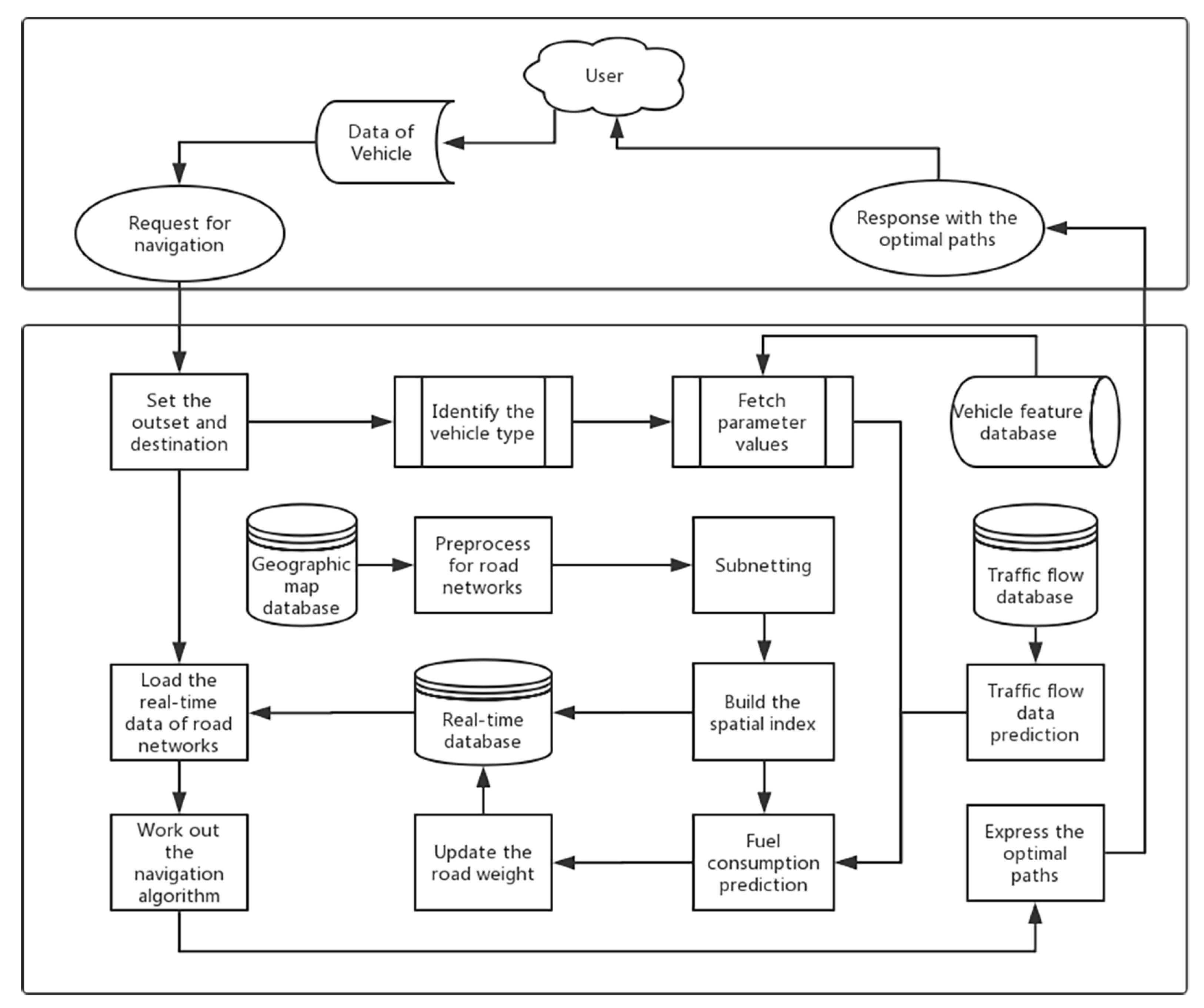
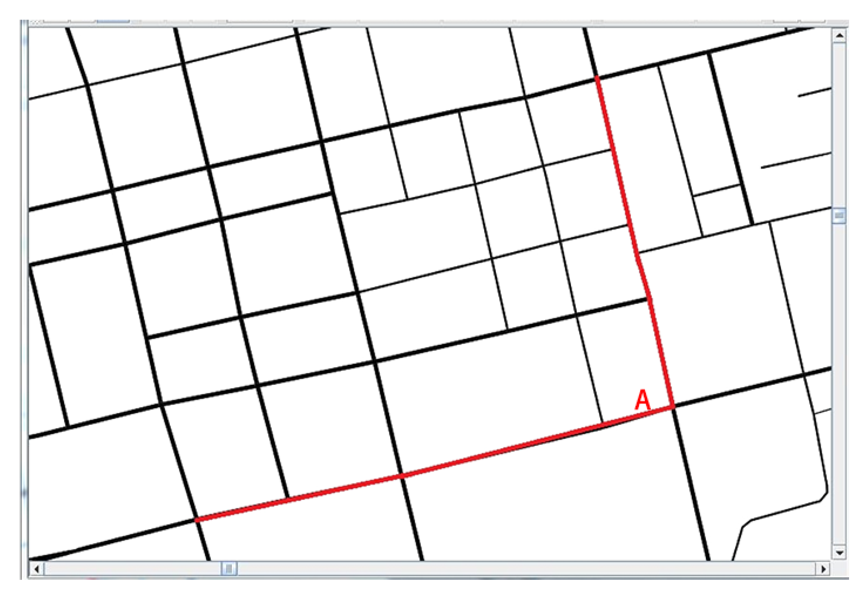
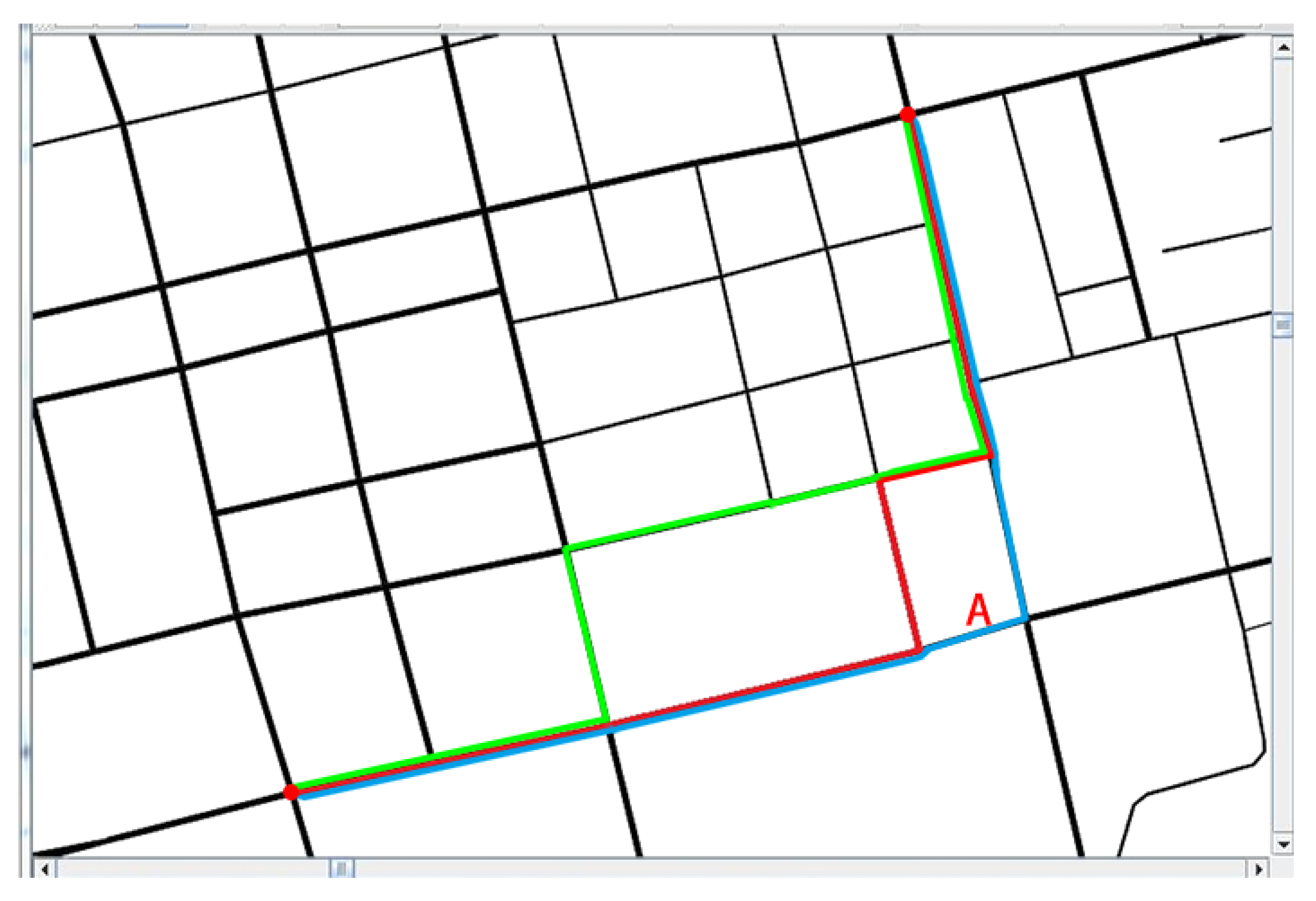
6. Low-Carbon-Emission-Oriented Navigation Method
7. Experimental Results
7.1. Experimental Framework
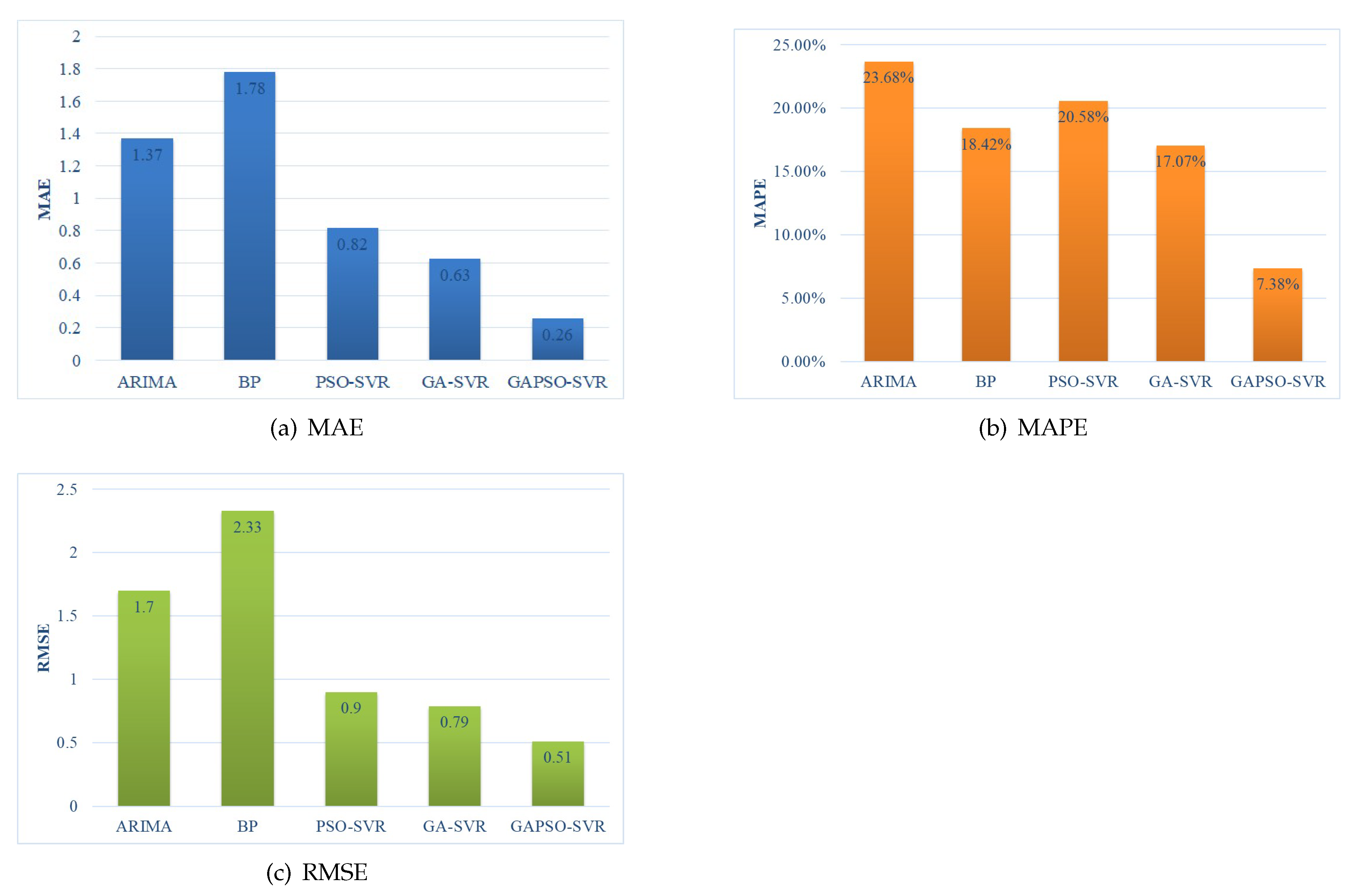
7.2. Evaluation of the Traffic Flow Prediction Model
7.3. Evaluation of the Low-Carbon-Emission-Oriented Navigation Algorithm
8. Conclusions
Author Contributions
Funding
Conflicts of Interest
References
- Alkhammash, E.H.; Jussila, J.; Lytras, M.D.; Visvizi, A. Annotation of smart cities Twitter micro-contents for enhanced citizen engagement. IEEE Access 2019, 7, 116267–116276. [Google Scholar] [CrossRef]
- Lytras, M.D.; Visvizi, A.; Sarirete, A. Clustering smart city services: Perceptions, expectations, responses. Sustainability 2019, 11, 1669. [Google Scholar] [CrossRef]
- Visvizi, A.; Lytras, M.D.; Damiani, E.; Mathkour, H. Policy making for smart cities: Innovation and social inclusive economic growth for sustainability. J. Sci. Technol. Policy Manag. 2018, 9, 126–133. [Google Scholar] [CrossRef]
- Visvizi, A.; Lytras, M.D. Rescaling and refocusing smart cities research: From mega cities to smart villages. J. Sci. Technol. Policy Manag. 2018, 9, 134–145. [Google Scholar] [CrossRef]
- Lytras, M.D.; Visvizi, A. Who uses smart city services and what to make of it: Toward interdisciplinary smart cities research. Sustainability 2018, 10, 1998. [Google Scholar] [CrossRef]
- Liang, Z.; Wakahara, Y. City traffic prediction based on real-time traffic information for intelligent transport systems. In Proceedings of the 2013 13th International Conference on ITS Telecommunications (ITST), Tampere, Finland, 5–7 November 2013; IEEE: Piscataway, NJ, USA, 2013; pp. 378–383. [Google Scholar]
- Deng, R.; Liang, H. Whether to charge an electric vehicle or not? A near-optimal online approach. In Proceedings of the 2016 IEEE Power and Energy Society General Meeting (PESGM), Boston, MA, USA, 17–21 July 2016; IEEE: Piscataway, NJ, USA, 2016; pp. 1–5. [Google Scholar]
- Wang, X.; Ning, Z.; Wang, L. Offloading in Internet of vehicles: A fog-enabled real-time traffic management system. IEEE Trans. Ind. Inform. 2018, 14, 4568–4578. [Google Scholar] [CrossRef]
- Tagami, K.; Takahashi, T.; Takahashi, F. “Electro Gyro-Cator” New Inertial Navigation System for Use in Automobiles; Society of Automotive Engineers: Warrendale, PA, USA, 1983; pp. 1103–1114. [Google Scholar]
- Arai, M.; Nakamura, Y.; Shirakawa, I. History of development of map-based automotive navigation system ‘honda electro gyrocator’. In Proceedings of the 2015 ICOHTEC/IEEE International History of High-Technologies and Their Socio-Cultural Contexts Conference (HISTELCON), Tel-Aviv, Israel, 18–19 August 2015; IEEE: Piscataway, NJ, USA, 2015; pp. 1–4. [Google Scholar]
- Bicego, J. Method and System for Automatically Updating Traffic Incident Data for In-Vehicle Navigation. U.S. Patent 8,155,865, 10 April 2012. [Google Scholar]
- Kumar, S.V. Traffic flow prediction using Kalman filtering technique. Procedia Eng. 2017, 187, 582–587. [Google Scholar] [CrossRef]
- Zhao, J.; Sun, S. High-order Gaussian process dynamical models for traffic flow prediction. IEEE Trans. Intell. Transp. Syst. 2016, 17, 2014–2019. [Google Scholar] [CrossRef]
- Yang, B.; Sun, S.; Li, J.; Lin, X.; Tian, Y. Traffic flow prediction using LSTM with feature enhancement. Neurocomputing 2019, 332, 320–327. [Google Scholar] [CrossRef]
- Luo, X.; Li, D.; Zhang, S. Traffic flow prediction during the holidays based on DFT and SVR. J. Sens. 2019, 2019, 1–10. [Google Scholar] [CrossRef]
- Yu, E.S.; Chen, C.Y.R. Traffic prediction using neural networks. In Proceedings of the GLOBECOM’93, IEEE Global Telecommunications Conference, Houston, TX, USA, 29 November–2 December 1993; IEEE: Piscataway, NJ, USA, 1993; pp. 991–995. [Google Scholar]
- Messai, N.; Thomas, P.; Lefebvre, D.; El Moudni, A. A neural network approach for freeway traffic flow prediction. In Proceedings of the International Conference on Control Applications, Glasgow, UK, 18–20 September 2002; IEEE: Piscataway, NJ, USA, 2002; Volume 2, pp. 984–989. [Google Scholar]
- Lopez-Garcia, P.; Onieva, E.; Osaba, E.; Masegosa, A.D.; Perallos, A. A Hybrid Method for Short-Term Traffic Congestion Forecasting Using Genetic Algorithms and Cross Entropy. IEEE Trans. Intell. Transp. Syst. 2016, 17, 557–569. [Google Scholar] [CrossRef]
- Feng, X.; Ling, X.; Zheng, H.; Chen, Z.; Xu, Y. Adaptive Multi-Kernel SVM With Spatial-Temporal Correlation for Short-Term Traffic Flow Prediction. IEEE Trans. Intell. Transp. Syst. 2019, 20, 2001–2013. [Google Scholar] [CrossRef]
- Li, L.; Qin, L.; Qu, X.; Zhang, J.; Wang, Y.; Ran, B. Day-ahead traffic flow forecasting based on a deep belief network optimized by the multi-objective particle swarm algorithm. Knowl. Based Syst. 2019, 172, 1–14. [Google Scholar] [CrossRef]
- Raja, P.; Pugazhenthi, S. Optimal path planning of mobile robots: A review. Int. J. Phys. Sci. 2012, 7, 1314–1320. [Google Scholar] [CrossRef]
- McGinty, L.; Smyth, B. Personalised route planning: A case-based approach. In Proceedings of the European Workshop on Advances in Case-Based Reasoning, Trento, Italy, 6–9 September 2000; Springer: Berlin/Heidelberg, Germany, 2000; pp. 431–443. [Google Scholar]
- Nie, Y.M.; Wu, X. Shortest path problem considering on-time arrival probability. Transp. Res. Part Methodol. 2009, 43, 597–613. [Google Scholar] [CrossRef]
- Grote, M.; Williams, I.; Preston, J.; Kemp, S. A practical model for predicting road traffic carbon dioxide emissions using Inductive Loop Detector data. Transp. Res. Part Transp. Environ. 2018, 63, 809–825. [Google Scholar] [CrossRef]
- Nocera, S.; Ruiz-Alarcn-Quintero, C.; Cavallaro, F. Assessing carbon emissions from road transport through traffic flow estimators. Transp. Res. Part Emerg. Technol. 2018, 95, 125–148. [Google Scholar] [CrossRef]
- Yang, Z.; Peng, J.; Wu, L.; Ma, C.; Zou, C.; Wei, N.; Zhang, Y.; Liu, Y.; Andre, M.; Li, D.; et al. Speed-guided intelligent transportation system helps achieve low-carbon and green traffic: Evidence from real-world measurements. J. Clean. Prod. 2020, 268, 122230. [Google Scholar] [CrossRef]
- Deng, Y.; Chen, Y.; Zhang, Y.; Mahadevan, S. Fuzzy Dijkstra algorithm for shortest path problem under uncertain environment. Appl. Soft Comput. 2012, 12, 1231–1237. [Google Scholar] [CrossRef]
- Pan, J.; Popa, I.S.; Zeitouni, K.; Borcea, C. Proactive vehicular traffic rerouting for lower travel time. IEEE Trans. Veh. Technol. 2013, 62, 3551–3568. [Google Scholar] [CrossRef]
- Xiao, Y.; Zhao, Q.; Kaku, I.; Xu, Y. Development of a fuel consumption optimization model for the capacitated vehicle routing problem. Comput. Oper. Res. 2012, 39, 1419–1431. [Google Scholar] [CrossRef]
- Bowyer, D.P.; Akcelik, R.; Biggs, D.C. Fuel Consumption Analyses for Urban Trafic Management. ITE J. 1986, 56, 31–34. [Google Scholar]
- Hammarstrom, U.; Eriksson, J.; Karlsson, R.; Yahya, M.R. Rolling resistance model, fuel consumption model and the traffic energy saving potential from changed road surface conditions. Vti Rapp. 2012, 8, 14–16. [Google Scholar]
- Barth, M.; An, F.; Younglove, T.; Scora, G.; Levine, C.; Ross, M.; Wenzel, T. The Development of a Comprehensive Modal Emissions Model; NCHRP Web-Only Documents; NCHRP: Washington, DC, USA, 2000; Volume 122.
- Barth, M.; Boriboonsomsin, K. Real-world carbon dioxide impacts of traffic congestion. Transp. Res. Rec. 2008, 2058, 163–171. [Google Scholar] [CrossRef]
- Demir, E.; Bektas, T.; Laporte, G. A comparative analysis of several vehicle emission models for road freight transportation. Transp. Res. Part Transp. Environ. 2011, 16, 347–357. [Google Scholar] [CrossRef]
- Demir, E.; Bektash, T.; Laporte, G. An adaptive large neighborhood search heuristic for the pollution-routing problem. Eur. J. Oper. Res. 2012, 223, 346–359. [Google Scholar] [CrossRef]
- Li, H.; Wang, Y.; Xu, X.; Qin, L.; Zhang, H. Short-term passenger flow prediction under passenger flow control using a dynamic radial basis function network. Appl. Soft Comput. 2019, 83, 105620. [Google Scholar] [CrossRef]
- Gu, Y.; Lu, W.; Xu, X.; Qin, L.; Shao, Z.; Zhang, H. An Improved Bayesian Combination Model for Short-Term Traffic Prediction With Deep Learning. IEEE Trans. Intell. Transp. Syst. 2019, 21, 1332–1342. [Google Scholar] [CrossRef]
- Bi, J.; Bennett, K.P. A geometric approach to support vector regression. Neurocomputing 2003, 55, 79–108. [Google Scholar] [CrossRef]
- Wang, M.; Wang, L.; Xu, X.; Qin, Y.; Qin, L. Genetic Algorithm-Based Particle Swarm Optimization Approach to Reschedule High-Speed Railway Timetables: A Case Study in China. J. Adv. Transp. 2019. [Google Scholar] [CrossRef]
- Mainali, M.K.; Mabu, S.; Yu, S.; Eto, S.; Hirasawa, K. Dynamic optimal route search algorithm for car navigation systems with preferences by dynamic programming. IEEJ Trans. Electr. Electron. Eng. 2011, 6, 14–22. [Google Scholar] [CrossRef]
- Yang, X.; Luo, S.; Gao, K.; Qiao, T.; Chen, X. Application of Data Science Technologies in Intelligent Prediction of Traffic Congestion. J. Adv. Transp. 2019, 2019, 2915369. [Google Scholar] [CrossRef]
- Zeng, M.; Yang, X.; Wang, M.; Xu, B. Application of Angle Related Cost Function Optimization for Dynamic Path Planning Algorithm. Algorithms 2018, 11, 127. [Google Scholar] [CrossRef]
- Lv, B.; Xu, H.; Wu, J.; Tian, Y.; Zhang, Y.; Zheng, Y.; Yuan, C.; Tian, S. LiDAR-enhanced connected infrastructures sensing and broadcasting high-resolution traffic information serving smart cities. IEEE Access 2019, 7, 79895–79907. [Google Scholar] [CrossRef]


| Parameter | Interpretation | Value |
|---|---|---|
| fuel-to-air mass ratio | 1 | |
| K | engine friction factor | 0.2 |
| g | gravity acceleration | 9.81 |
| coefficient of aerodynamic drag | 0.7 | |
| air density | 1.2041 | |
| coefficient of rolling resistance | 0.01 | |
| efficiency of mechanical transmission | 0.4 | |
| efficiency of the engine | 0.9 | |
| road slope angle | 0 | |
| energy conversion value | 737 |
| Parameter | Interpretation | Value |
|---|---|---|
| m | vehicle net weight | 1495 kg |
| load weight | 300 kg | |
| N | engine speed | 33 rpm |
| V | engine displacement | 1.395 L |
| A | the frontal surface area | 2.721 m |
| fuel calorific value | 43 |
| Item | Germany Cologne |
|---|---|
| Longitude and latitude | 6.762104, 50.772113, 7.223816, 51.127596 |
| SUMO boarders | 0.00, 0.00, 32765.27, 34478.96 |
| Traffic flow time line | 6:00–8:00 a.m. |
| Node number | 30,354 |
| Road number | 68,642 |
| Road connection number | 190,630 |
| Route ID | Head | Tail | Weight | Time Consumption |
|---|---|---|---|---|
| 238549234#3 | 1942418153 | 1942483552 | 0.0201 | 37.98 |
| 238549234#4 | 1942483552 | 445359497 | 0.0254 | 49.10 |
| 238549234#5 | 445359497 | 1996182197 | 0.0413 | 61.41 |
| 238549234#6 | 1996182197 | 445359806 | 0.0165 | 32.43 |
| 188982766#1 | 445359806 | 445360200 | 0.0232 | 40.39 |
| 188982766#2 | 445360200 | 1942418274 | 0.0121 | 26.65 |
| 188982766#3 | 1942418274 | 1996182256 | 0.0098 | 24.87 |
| 188982766#4 | 1996182256 | 2613699165 | 0.0176 | 35.99 |
| 188982766#5 | 2613699165 | 445359828 | 0.0165 | 34.09 |
| Route ID | Head | Tail | Weight | Time Consumption |
|---|---|---|---|---|
| … the same as Table 4 … | ||||
| 238549234#6 | 1996182197 | 445359806 | 0.0451 | 142.73 |
| … the same as Table 4 … | ||||
| Route ID | Head | Tail | Weight | Time Consumption |
|---|---|---|---|---|
| 238549234#3 | 1942418153 | 1942483552 | 0.0201 | 37.98 |
| 238549234#4 | 1942483552 | 445359497 | 0.0254 | 49.10 |
| 238549234#5 | 445359497 | 1996182197 | 0.0413 | 61.41 |
| -188982779#4 | 1996182197 | 445359806 | 0.0270 | 63.79 |
| 37932733#10 | 445359806 | 445360200 | 0.0170 | 33.22 |
| 188982766#2 | 445360200 | 1942418274 | 0.0121 | 26.65 |
| 188982766#3 | 1942418274 | 1996182256 | 0.0098 | 24.87 |
| 188982766#4 | 1996182256 | 2613699165 | 0.0176 | 35.99 |
| 188982766#5 | 2613699165 | 445359828 | 0.0165 | 34.09 |
© 2020 by the authors. Licensee MDPI, Basel, Switzerland. This article is an open access article distributed under the terms and conditions of the Creative Commons Attribution (CC BY) license (http://creativecommons.org/licenses/by/4.0/).
Share and Cite
Peng, T.; Yang, X.; Xu, Z.; Liang, Y. Constructing an Environmental Friendly Low-Carbon-Emission Intelligent Transportation System Based on Big Data and Machine Learning Methods. Sustainability 2020, 12, 8118. https://doi.org/10.3390/su12198118
Peng T, Yang X, Xu Z, Liang Y. Constructing an Environmental Friendly Low-Carbon-Emission Intelligent Transportation System Based on Big Data and Machine Learning Methods. Sustainability. 2020; 12(19):8118. https://doi.org/10.3390/su12198118
Chicago/Turabian StylePeng, Tu, Xu Yang, Zi Xu, and Yu Liang. 2020. "Constructing an Environmental Friendly Low-Carbon-Emission Intelligent Transportation System Based on Big Data and Machine Learning Methods" Sustainability 12, no. 19: 8118. https://doi.org/10.3390/su12198118
APA StylePeng, T., Yang, X., Xu, Z., & Liang, Y. (2020). Constructing an Environmental Friendly Low-Carbon-Emission Intelligent Transportation System Based on Big Data and Machine Learning Methods. Sustainability, 12(19), 8118. https://doi.org/10.3390/su12198118