Basic Soil Data Requirements for Process-Based Crop Models as a Basis for Crop Diversification

Abstract

Data from global soil databases are increasingly used for crop modelling, but the impact of such data on simulated crop yield has not been not extensively studied. Accurate yield estimation is particularly useful for yield mapping and crop diversification planning. In this article, available soil profile data across Sri Lanka were harmonised and compared with the data from two global soil databases (Soilgrids and Openlandmap). Their impact on simulated crop (rice) yield was studied using a pre-calibrated Agricultural Production Systems Simulator (APSIM) as an exemplar model. To identify the most sensitive soil parameters, a global sensitivity analysis was performed for all parameters across three datasets. Different soil parameters in both global datasets showed significantly (p < 0.05) lower and higher values than observed values. However, simulated rice yields using global data were significantly (p < 0.05) higher than from observed soil. Due to the relatively lower sensitivity to the yield, all parameters except soil texture and bulk density can still be supplied from global databases when observed data are not available. To facilitate the wider application of digital soil data for yield simulations, particularly for neglected and underutilised crops, nation-wide soil maps for 9 parameters up to 100 cm depth were generated and made available online.

1. Introduction

With the growing concern about climate change and food security, process-based crop models have been used to aid decisions at local, regional and global scales [1,2]. Traditional agronomic experiments are time-consuming and expensive, but crop performance simulations allow evaluation of the potential of crops and crop varieties in different geographic locations under different agro-climatic environments [3]. Crop modelling approaches are also used in on-farm decision making, studying nutrient dynamics [4], plant breeding [5], sensitivity of crops to changing climates [1] and policy-making [2]. Crop modelling is a particularly useful tool for understanding the likely productivity of crops in different environments. It has been recently suggested that crop modelling can be used to provide evidence for crop diversification in areas that are affected by climate change [6,7]. Simulating the crop yield is particularly cumbersome for these crops as detailed field data are rarely available. Modelling the performance of these crops however can benefit from extensive data being available for major crops.

To understand the genotype–environment (G × E) interaction in crop models and capture agronomic reality, the availability of good quality environmental data is essential. Currently, spatial and temporal variability in soil and climatic factors can be captured in crop models [8] and studies have shown that crop models are sensitive to variation and therefore, capturing these dynamics is important in delivering more accurate estimates. For example, using global gridded crop models, Folberth et al. [9] reported that the soil type has a higher impact on crop yield than the interannual yield variability due to weather. This is because soil texture has dynamic interactions with precipitation and plant-available water content to buffer soil water holding capacity [9]. Others have reported the importance of accurate soil data and their impact on yield simulations [8,10]. Furthermore, the yield change under climate change can be either positive or negative depending on the type of soil [9]. Therefore, reliable and accurate soil data are essential to minimise the uncertainty in yield simulations.

Understanding the sensitivity of simulated yield to all input parameters in process-based crop models is crucial in improving productivity. Climate data have been increasingly available in local, regional and global databases and through remote sensing and reanalysis methods [11]. However, the unavailability of observed soil data is still a challenge for crop model simulations [12].

Soil information in most countries is traditionally made available through semi-detailed soil series maps that show the distribution of soils through sampled profiles or expert knowledge. The focus in these inventories is to provide soil types rather than individual soil properties, e.g., pH, texture, etc. [13]. Additionally, these profiles often reflect information at different depths as soil horizons vary from one location to another. Another major limitation of conventional soil mapping is the scale at which soil information is aggregated and the limitation of such data to provide finer scale soil property information. Although these data are very useful in many areas including regional planning, they needs extensive work in terms of digitisation, harmonisation of depths and estimation of missing parameters before they can be used in crop models.

At the global level, few databases provide soil data at different geographic scales. The Harmonized World Soil Database (HWSD) is a 30 arc-second raster database [14] and the International Soil Reference and Information Centre—World Inventory of Soil Emission Potentials (ISRIC–WISE) contains generalised soil data in a 5 by 5 arc-minute resolution [15]. The World Soil Information Service (WoSIS) database provides data in point, polygon and grid formats that are useful for mapping [16].

Following several attempts to harmonise soil profiles and profile data at the global level (Harmonized World Soil Database, 2020; [17]), maps of soil properties at a finer spatial resolution have recently been developed using digital soil mapping techniques. Soilgrids and Openlandmap are examples of such attempts to provide free to access interpolated soil property information in geospatial formats [18,19]. The aim is to provide an automated soil property mapping framework that distributes global soil information with a reasonable degree of accuracy and scale. This information could potentially be used for finer scale insight generation regarding agricultural productivity [6]. Both Soilgrids and Openalandmap databases produce predictions with various degrees of accuracy between locations and properties depending on the density of samples and analytical techniques. However, the application of these data for crop modelling using process-based modes such as Agricultural Production Systems Simulator (APSIM) [2] is not studied. Nevertheless, since their data are provided at a finer resolution (close to density of observed field data) there is a potential to use this data for crop simulation modelling.

Few attempts have been made to use global soil data in yield simulations. Soil daTA Retrieval Tool (START) prepares input data for crop models using Soilgrids database [20]. Additionally, a digital database [12] is developed using Soilgrids data to prepare soil input files for Decision Support System for Agro-technology Transfer (DSSAT) crop model [21]. However, assessing the crop modelling performance with observed data versus globally provided data is an area that remains unexplored. Evaluating the impact of such data on the crop modelling outputs provides a primer to wider utilisation of open data for the benefit of all stakeholders interested in agricultural diversification.

Other than issues such as reliability and formats, assessment of the impact of individual input parameters in crop simulation modelling is also important. Although sensitivity analysis methods that use all input variables (global sensitivity analysis methods) are generally computationally expensive, their use in understanding the influence of input parameter space of models with many variables (e.g., crop modelling) is crucial. Another important advantage of using global methods in estimating the sensitivity of all parameters is understanding the interactions that exist within the parameter space. Global methods have been used to ascertain the sensitivity of environmental parameters in relation to yield. For example, Varella et al. [22] studied the global sensitivity of wheat yield in relation to different soil, climate and crop conditions and Vanuytrecht et al. [23] employed the global sensitivity analysis for determining the yield response to water availability. Soil parameter sensitivity estimation is therefore essential in understanding the utility of such data in crop modelling.

Once the output yield is properly estimated and validated, extrapolation of crop simulation modelling results can generate valuable information regarding crop production in current and future climates. Mapping the yield estimates using globally available datasets is becoming widespread. For example, fine resolution data have been used in regional level crop modelling in the global yield gap atlas project (GYGA—http://www.yieldgap.org/). With the increased popularity of web-based decision support systems such as LANDSUPPORT (https://www.landsupport.eu/) [24], the importance of harmonising conventional soil data and examining their efficiency in modelling becomes more evident [6]. Therefore, in this study, we compared the observed soil data with global data (Soilgrids and Openlandmap) in simulating yield using an exemplar crop model to determine the fitness of global datasets for regional and possibly local decision making. The sensitivity of yield to each soil parameter was also evaluated based on a harmonised soil dataset across Sri Lanka that was developed in this study to confirm the relative significance of each parameter and database in yield simulations. Since the available global soil databases did not capture the spatial variability of soil properties in the country, interpolated soil maps were created and made available using the observed data as an alternative database to be used in process-based crop models.

2. Materials and Methods

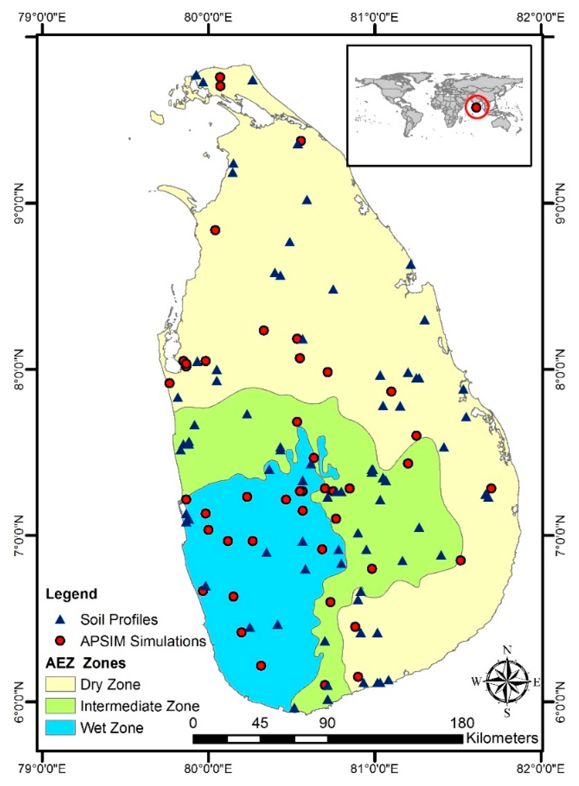
2.1. Study Area

This study was conducted in Sri Lanka, which is a tropical island in the Indian ocean, located between 5° and 10° north latitude. Therefore, seasonal temperature variation is not observed in the country. The mean annual temperature of the country varies from 16 °C in the central highlands to 27 °C in the coastal plains due to the altitudinal changes. The mean annual rainfall ranges from below 900 mm in the dry zone to above 5000 mm in the wet zone. Rainfall follows a bi-modal distribution with two peaks centered in March–April and October–November [25]. The country is divided into three major climatic zones according to the annual rainfall amount; the dry zone (annual rainfall <1750 mm) that covers the east, northern and south-east part of the country, the wet zone (>2500 mm rainfall annually) in the central and south-west regions and the intermediate zone (1750–2500 mm annual rainfall) separating the two (Figure 1). The country is divided into three altitudinal classes as Low country (<300 m), Mid country (300–900 m) and Up country (>900 m) [25]. Due to the diversity of climatic conditions, a wide range of soil properties can be observed in Sri Lanka [26].

2.2. Observed Soil Data

Soil profile data were obtained from the SRICANSOL project [27,28,29] which is the most comprehensive and up-to-date soil database in Sri Lanka that describes taxonomic, physical and chemical properties of 110 georeferenced benchmark soil series in the country. Moreover, 12 georeferenced benchmark soil profiles for the northern region which are not included in the SRICANSOL project were obtained from Mapa [30]. The altitude of sample collection sites ranged from 0.5 m to 2200 m above mean sea level. The distribution of sampling locations that were used in this study is shown in Figure 1. These locations cover almost all the land use types in Sri Lanka including agricultural fields, bare lands, plantations, forests and urban areas [26].

The selected properties were bulk density (BD—g cm^–3), sand content (%), silt content (%), clay content (%), pH (in water), cation exchange capacity (CEC—cmol + kg⁻¹), organic carbon (%), volumetric water content (VWC) at 0.33 bars pressure (VWC33) and 15 bars pressure (VWC1500). These are the basic soil properties required for APSIM simulations. Detailed analysis methods are available in Mapa et al. [29].

From the profile data, 44 locations that contained all the required properties up to 200 cm depth were used for detailed comparison and APSIM simulations (Figure 1). Among them, 18 locations were in the dry zone (DZ), 11 in the intermediate zone (IZ) and 15 in the wet zone (WZ).

2.3. Global Soil Data

Data from two digital soil databases were used in this study: Soilgrids [18] and Openlandmap [13]. The Soilgrids database uses 150,000 profile datapoints from the World Soil Information Service (WoSIS) and other sources, while Openlandmap uses 350,000 field observations of soil types based on a compiled United States Department of Agriculture, (USDA) database (National Cooperative Soil Survey, 2020) and various other sources to predict property maps using machine learning techniques [18]. Both of these databases provide important variables needed for crop modelling such as bulk density, soil texture, organic matter content and pH at finer scales. While Openlandmap provides soil water content at 33 kPa, Soilgrids does not provide such information; cation exchange capacity is not available in Openlandmap.

2.4. Calculations and Estimation of Missing Parameters

In both the SRICANSOL and Soilgrids databases, soil pH is based on a 1:2.5 soil water ratio. In Openlandmap, the ratio of 1:1 was used to determine soil pH. However, modern soil classifications, databases and crop models use the ratio of 1:5, which is defined according to the international standards for soil pH determination (ISO 10390:2005). Therefore, soil pH in 1:2.5 and 1:1 ratios of water (W) were converted to 1:5 following the methods developed by Kabała et al. [31] (Equation (1)) and Libohova et al. [32] (Equation (2)), respectively.

pH 1:5W = 0.14 + 0.99 × pH 1:2.5W

(1)

pH 1:5W = −0.51 + 1.06 × pH 1:1W

(2)

Soil moisture information was not available in Soilgrids while VWC33 is available in the Openlandmap database. Therefore, volumetric water content at 0.33 bars level (VWC33) and 15 bars (VWC1500) were calculated using the pedotransfer functions developed by Gunarathna et al. [33] from the SRICANSOL dataset (Equations (3) and (4)). Parallel to the crop model parameters, VWC33 and VWC1500 were labelled as drainage upper limit (DUL) and wilting point (LL15), respectively.

VWC33 (DUL) = 0.4357 − 0.0035 × Sand%

(3)

VWC1500 (LL15) = 0.3426 − 0.003 × Sand%

(4)

Following the APSoil parameter estimation protocol [34], the soil moisture limit to which soil can dry by evaporation (AirDry − AD) was calculated as 50% of the LL15 value in the top two layers (0–5 and 5–15 cm), 80% in the 15–30 cm layer and 100% for all other profiles. Saturation (SAT) was estimated for all the soils using porosity (PO) as follows.

PO = 1 − BD/TD

(5)

where 2.65 g cm⁻³ was used as TD (true density).

SAT = PO − e

(6)

A similar value of 0.05 was used for e in all the soils. The Soilgrids data are available for 7 standard depths: 0, 5, 15, 30, 60, 100 and 200 cm making 6 layers. Average soil properties over depth intervals (0–5, 5–15, 15–30, 30–60, 60–100 and 100–200 cm) were derived based on the weighted average of the depths using the trapezoidal rule (Equation (7)) [18].

$$\frac{1}{b-a}{{\displaystyle \int }}_a^{b}f\left(x\right)dx \approx \frac{1}{\left(b-a\right)}\frac{1}{2}{\displaystyle \sum }_{k=1}^{N-1}\left(x_{k+1}-x_k\right)\left(f\left(x_k\right)+f\left(x_{k+1}\right)\right)$$

(7)

Openlandmap contains soil data for 6 depths as 0, 10, 30, 60, 100 and 200 cm forming 5 layers, therefore, the weighted average within the depths was calculated. To avoid the effect of depth on simulated yield, the depths in both observed and Openlandmap data were standardised to 6 layers as 0–5, 5–15, 15–30, 30–60, 60–100 and 100–200 cm using equal-area quadratic smoothing splines. SplineTool v2 available at: http://www.asris.csiro.au [35] was used for the equal area spline process.

2.5. Yield Simulations

2.5.1. Crop

Rice was selected as the crop to simulate with both observed and global soil data because it is the major crop in Sri Lanka that covers 15% of the total area and 29% of agricultural lands in the year 2018 [36]. Rice is cultivated in all 25 administrative districts of the country in different amounts. We selected BG 357, a local improved rice variety with the maximum observed yield of 9.5 t ha⁻¹ (Department of Agriculture Sri Lanka—DOASL). The selected variety can be harvested within a three-and-a-half-month period. Out of nearly 75 known varieties, BG 357 accounted for 2.2% of total rice cultivated area in the 2017/2018 major growing season [36].

2.5.2. Crop Model

Many crop models require fair amount of soil information. In this study we chose the APSIM (Version 7.10) model as an exemplar crop model with extensive literature that is available for the APSIM rice module for Sri Lanka. APSIM contains a set of biophysical models that simulate different aspects of a cropping system. The plant models simulate crop phenology, organ development and physiological processes, assimilation and partitioning of biomass and response to abiotic stresses. Crop- or cultivar-specific genotypic information is needed to simulate crop performance. Evaporation, water movement and infiltration within profiles, runoff and cycling of different solutes can be simulated by soil models [2]. Daily minimum and maximum temperatures, solar radiation and rainfall are key weather inputs in APSIM. Crop management options allow simulation of a wide range of crop management practices including planting, fertiliser application and irrigation. Detailed descriptions of APSIM and supporting models are available at [2,37]. APSIM Oryza [38] simulates daily growth and development of rice. Rice growth responds to climate (radiation, temperature and rainfall), soil water supply (SoilWat model), and soil nitrogen (SoilN model) [39].

2.5.3. APSIM Simulations

Rice is cultivated as a rainfed crop in Sri Lanka during the major growing season which falls between October to March [40]. Direct seeding was selected as the planting method as it is the most common planting method in the country. The date of sowing was set as 1 November and the number of plants per seed bed (plants m⁻²) was 350 [40]. Generally, planting date varies across the country, but we used a fixed calendar date for all simulations to avoid the impact of sowing date on yield. Genetic coefficients of BG 357 generated by Zubair et al. [40] were added to the APSIM Oryza model while other crop parameters in the model (Version 7.10) were set to default. Recommended crop management standard procedures by the DOASL were adopted in the simulations. Maximum ponding depth was set as 50 mm during the 18 October–30 January period. Irrigation was enabled from 25 October to 31 January to top up the pond and ceased two weeks before harvesting. Following the DOASL recommendations for rainfed rice, urea was applied at 30 kg ha⁻¹ 3 weeks after planting (WAP), 70 kg ha⁻¹ at 5 WAP, 50 kg ha⁻¹ at 7 WAP and 30 kg ha⁻¹ at 8 WAP; 10 kg ha⁻¹ of rock phosphate was added at sowing. The field was assumed to be weed-, pest- and disease-free.

For the soil parameters, saturated flow-proportion of water above DUL which will drain to adjacent soil layers per day (SWCON) was set as 0.5 throughout all profiles. The proportion of initial organic carbon assumed to be inert (FInert) was 0.4 for 0–15 cm depths, 0.5 for 15–30 cm, 0.7 for 30–60 cm and 0.95 for the rest of the depths. The proportion of non-inert C in the microbial biomass pool (FBiom) was set as 0.035 for 0–15 cm depths, 0.03 for 15–30 cm, 0.015 for 30–100 depths and 0.01 for 100–200 cm [34]. Other parameters were set to default in APSIM (Version 7.10). All the soil files were prepared using APSoil (Version 7.20). Rice yield was simulated for a 30-year period (1980–2009).

Climate Data

The AgMERRA global gridded climate forcing dataset [41] (https://data.giss.nasa.gov/impacts/agmipcf/agmerra/) which contains all the required weather parameters for APSIM was used in simulations. Out of the several reanalysis climate databases that utilise comprehensive methods and covariates, AgMERRA was identified as a potential dataset to use in process-based crop models where observed data are not available [41,42,43] and has been used for APSIM simulations in Sri Lanka [40,44]. The effective resolution of different parameters in AgMERRA are 0.25° for rainfall, 0.5° for temperature and 1.0° for solar radiation. The selected 44 soil locations were covered by 34 different grids. Daily rainfall (mm), solar radiation (MJ m⁻² day⁻¹), minimum temperature (°C) and maximum temperature (°C) were used in simulations. The variation of rainfall and minimum and maximum temperature throughout the cropping period (1 November to 15 February) is shown in the Supplementary Materials (Figure S1).

2.6. Global Sensitivity Analysis

The variance-based global sensitivity analysis, developed by Sobol [45], is very useful due to its ability to partition model output variance for many input variables and their interactions in parameter space. However, Sobol’s method produces undesirable results in the presence of dependence among input variables. Recently, a new method based on game theory has been proposed to define indices to explain variance, such as Shapley’s function of attributing the importance of input variables (players) that are related to the Sobol indices, with applications in econometrics, multilinear extension of games and crop insurance [46,47,48,49]. Shapley values or Shapley effects, when calculated for a system with correlated regressors, provide consistent results [50]. Since there is a strong relationship between the soil variable (i.e., through pedotransfer functions), Shapley’s effects can be used to provide a reliable method for correctly ascertaining the impact of input space on the yield [51].

In this study, we calculated Shapley’s effect for all soil variables using a linear regression function of yield as the response variable. The ‘sensitivity’ extension package of the R statistical software [52] computes the Shapley effect for a linear Gaussian framework [53]. Using the vector of input variables coefficients and variance–covariance matrix of 30 linear emulators that were formed based on 30 years predicted yield and soil data, we computed the Shapley’s effect of soil parameters on the yield uncertainty. Since the linear gaussian method assumes normality, we log-transformed variables that showed strong non-normality in the Shapiro test [54,55].

Since Shapiro’s test of normality results were different for yields across the 30 years, we compared the result of the emulators with and without log-transforming yield. The result showed that using a log-transformed yield variable will produce more efficient models in terms of the standard deviation of residuals and adjusted R². We also log-transformed those independent variables that showed strong non-normality, including BD, SAT, OC and CEC.

2.7. Interpolation and Mapping

The spatial variability of soil properties is often captured through interpolation. The choice of interpolation technique, however, is important, as different interpolation methods can generate different results. Cross validation or the leaving-one-out technique is a powerful technique to compare the results of a wide range of interpolating techniques. The result of cross validation on each soil parameter showed that different techniques should be used for different parameters.

Stochastic techniques are the most suitable methods for prediction and mapping the spatial distribution of soil chemical properties [56,57,58]. For the soil chemical properties, Empirical Bayesian Kriging methods showed the smallest Root Mean Square Error (RMSE) values among the interpolation methods tested. On the other hand, for the soil physical properties, the Radial Basis Function (RBF) showed smaller RMSE values among the other interpolation methods. In some cases, deterministic interpolation was used due to non-existence of spatial dependence. Due to having fewer input requirements, it has been shown that RBF can be more usefully adopted by agronomists to map soil properties [59].

Due to the small number of samples, the bottom layer (100–200 cm) was excluded from the interpolation exercise. Therefore, interpolated maps were created for 5 standard depths as 0–5, 5–15, 15–30, 30–60 and 60–100 cm. All harmonised soil samples based on Mapa et al. [27,28,29,30] were used for interpolation mapping. Yield maps were interpolated using 44 locations (Figure 1) used in APSIM simulations. Empirical Bayesian Kriging was used as the interpolation method.

2.8. Evaluation

The efficiency of the simulated yield using different soil databases was evaluated both graphically and statistically. The error between datasets was measured using the Root Mean Square Error (RMSE) as follows (Equation (8)).

$$RMSE=\sqrt{\frac{{{\displaystyle \sum }}_{i=1}^n{(O_i-S_i)}^2}{n}}$$

(8)

where O is observed and S is simulated yield in n number of samples.

To compare the error between datasets with different scales, Normalized Root Mean Square Error (NRMSE) was performed (Equation (9)). The µ is the average of observed yields.

$$NRMSE=\frac{RMSE}{\mu }$$

(9)

Index of agreement, known as Wilmott index (d) measures the model prediction error between two datasets (Equation (10)). The value varies within 0 and 1, and zero indicates no agreement. The perfect match between datasets is indicated by 1.

$$d=1-\frac{{{\displaystyle \sum }}_{i=1}^n{\left(O_i-S_1\right)}^2}{{{\displaystyle \sum }}_{i=1}^n{(\left|S_i-\mu \right|+|O_i-\mu \left|\right)}^2},0\le d\le 1$$

(10)

3. Results

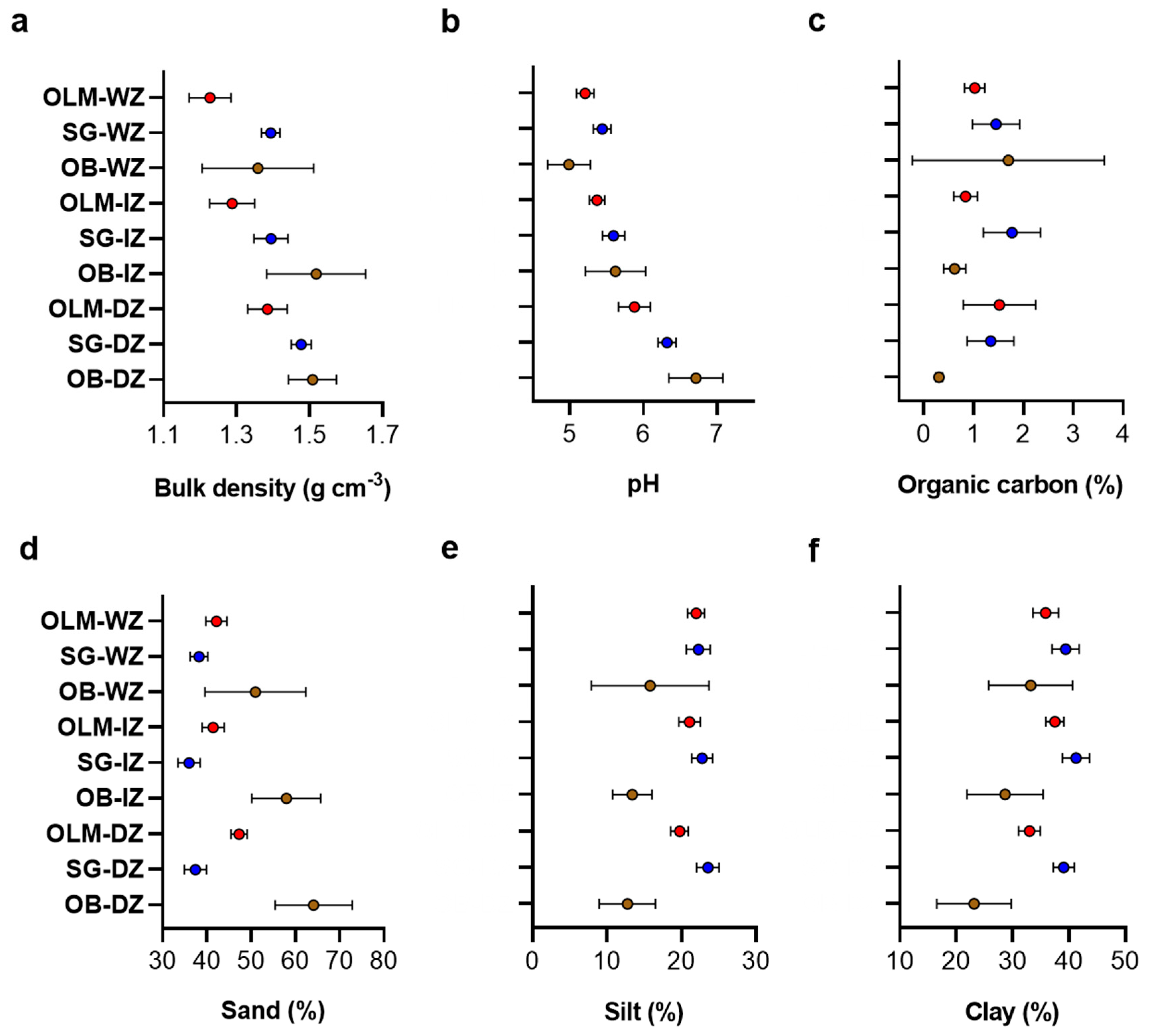
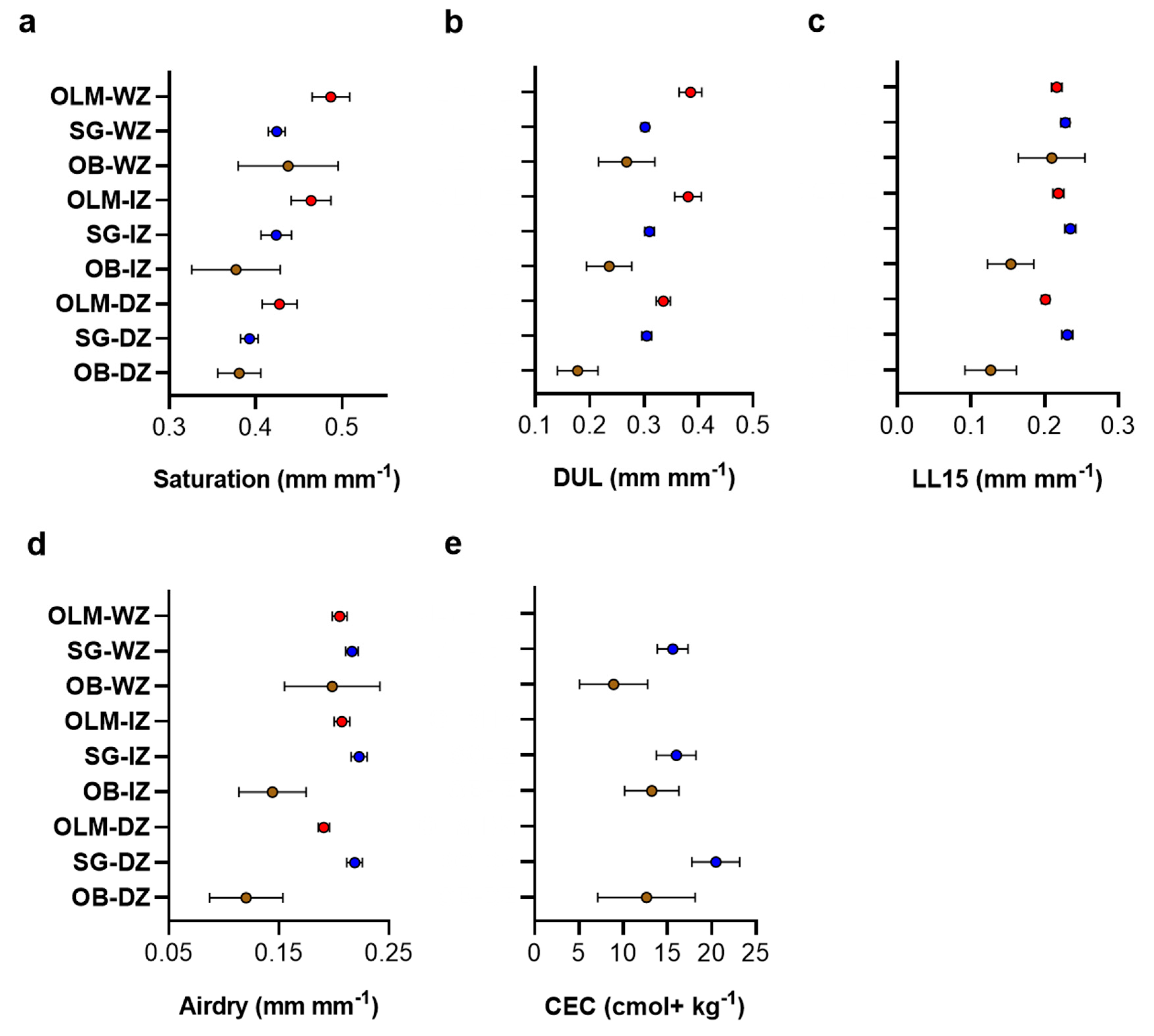
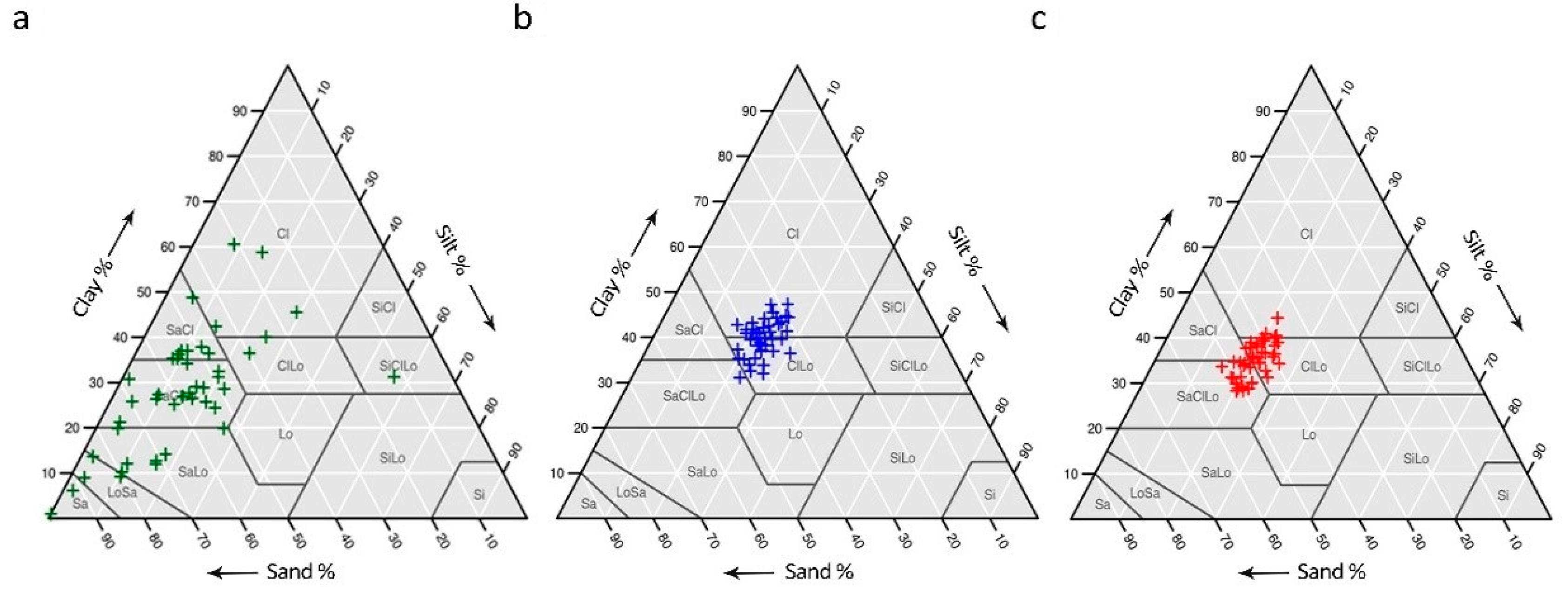
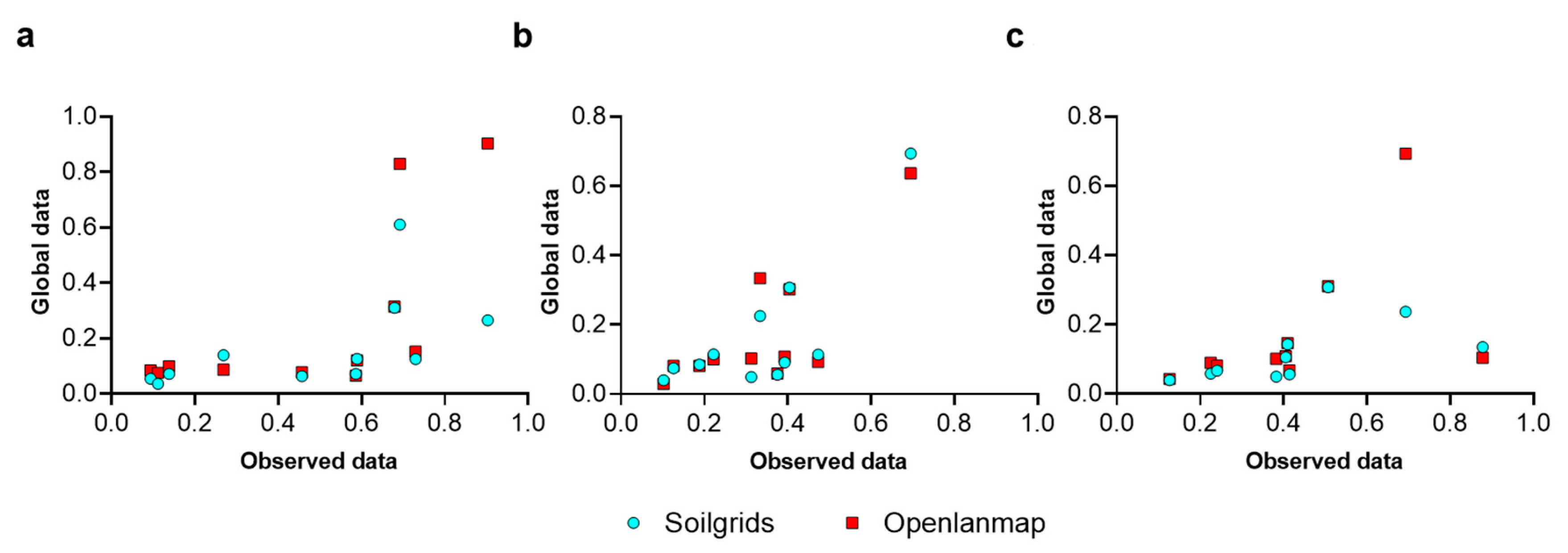
3.1. Comparison of Soil Properties in Different Climatic Zones

Of all observed soil parameters, the average pH, DUL, LL15 and AD (calculated) of the standard profiles were significantly (p < 0.05) different among climate zones indicating the high variability of soil properties in Sri Lanka (Figure 2 and Figure 3). In general, global data fail to capture the broad variability of observed soil data. The highest pH was observed from the dry zone, while soil moisture properties were higher in the wet zone. Bulk density, pH, CEC and SAT were significantly (p < 0.05) different among climatic zones in Soilgrids data. However, all the parameters except OC in Openlandmap data were significantly (p < 0.05) different among climatic zones.

All parameters except bulk density and saturation in Soilgrids were significantly (p < 0.05) different from the observed soil in the dry zone while all parameters were significantly (p < 0.05) different with Openlandmap data. In the intermediate zone, pH and CEC from Soilgrids and organic carbon and pH from Openlandmap were not significantly (p > 0.05) different from the observed soil data. In contrast with the two other regions, all parameters except pH, CEC and sand from Soilgrids and DUL from Openlandmap were not significantly (p > 0.05) different from observed data, indicating the higher agreement of global and observed soil data in the wet zone of the country. Two global datasets used in this study did not show a higher agreement as most of the parameters were significantly (p < 0.05) different from each other.

Organic carbon content in the dry zone and silt content in the wet zone were not significantly (p > 0.05) different among Soilgrids and Openlandmap while all other parameters were significantly (p < 0.05) different from each other. Sand, silt and clay content from global data in the dry zone were significantly (p < 0.05) different to the observed data, while Soilgrids data in the intermediate zone were significantly (p < 0.05) different in all three soil textural properties. Additionally, sand content in the wet zone was significantly different in Soilgrids data when compared with observed data. The discrepancies in both bulk density and textural values directly affect SAT, DUL, LL15 and AD since they were calculated using pedotransfer functions.

Textural classes of observed soils showed a comparatively higher diversity than global soils (Figure 4). Observed soils were distributed over 8 textural classes. However, most of the observed soils contained coarse fragments (sandy clay loam, sandy clay, sandy loam). In contrast, global soils were mainly distributed among 2–3 textural classes with smaller particles (clay and clay loam soils).

Except for cation exchange capacity, all other parameters in observed soil showed a comparatively higher coefficient of variation (CV) in intermediate and wet zones (Figure 2, Figure 3 and Figure 5). Except for a few points, all other parameters in Soilgrids and Openlandmap showed relatively lower CV values of less than 0.4 (Figure 5). This shows that except for sand, BD and pH, both Soilgrids and Openlandmap tend to overestimate the value and Soilgrids fails to capture the variation that exists in the observed data in all cases for all zones.

When considering 6 standard depths, the highest average bulk density was reported from observed soils. The minimum global bulk density data was 0.96 g cm⁻³ in all the depths and locations, while the lowest observed bulk density was 0.3 g cm⁻³ which occurs in a Silty clay loam soil in the wet zone (Madabokka series). Soil pH was slightly acidic in global databases while it ranged from acidic (2.37) to alkaline (8.27) in observed soil. Summary statistics of all three databases are given in

Table 1. Summary statistics of observed, Soilgrids and Openlandmap databases for selected locations for six standard depths.

Parameter		Observed	Soilgrids	Openlandmap
BD (g cm–3)	Mean	1.43 ± 0.23	1.38 ± 0.09	1.28 ± 0.13
	Range	0.30–1.82	1.08–1.55	0.96–1.53
OC (%)	Mean	1.13 ± 2.13	2.22 ± 1.58	1.65 ± 1.23
	Range	0.01–16.81	0.00–10.00	0.00–6.58
pH	Mean	5.79 ± 0.97	5.81 ± 0.45	5.46 ± 0.44
	Range	2.37–8.27	5.09–6.92	4.68–6.81
CEC (cmol(+) kg−1)	Mean	11.33 ± 8.21	18.48 ± 5.07	-
	Range	0.78–51.49	10.00–35.00	-
Sand (%)	Mean	61.20 ± 19.54	38.83 ± 4.84	45.54 ± 5.29
	Range	3.70–99.00	27.00–50.00	33.50–58.12
Silt (%)	Mean	13.66 ± 9.59	23.51 ± 2.88	21.25 ± 2.57
	Range	0.00–62.07	16.00–31.00	14.50–28.56
Clay (%)	Mean	25.13 ± 14.26	37.65 ± 4.90	33.21 ± 4.92
	Range	1.00–67.35	26.00–48.50	20.28–46.00
SAT (mm mm−1)	Mean	0.409 ± 0.089	0.429 ± 0.036	0.467 ± 0.049
	Range	0.263–0.836	0.365–0.544	0.373–0.589
DUL (mm mm−1)	Mean	0.220 ± 0.095	0.300 ± 0.017	0.356 ± 0.041
	Range	0.045–0.423	0.261–0.341	0.274–0.465
LL15 (mm mm−1)	Mean	0.162 ± 0.083	0.226 ± 0.015	0.206 ± 0.016
	Range	0.017–0.350	0.193–0.262	0.168–0.242
AD (mm mm−1)	Mean	0.129 ± 0.076	0.182 ± 0.056	0.166 ± 0.052
	Range	0.009–0.350	0.096–0.262	0.084–0.242

Note: BD = bulk density, OC = organic carbon, CEC = cation exchange capacity, SAT = saturation, DUL = drainage upper limit, LL15 = wilting point and AD = soil moisture limit to which soil can dry by evaporation. Values of 6 standard depths were used in this table.

.

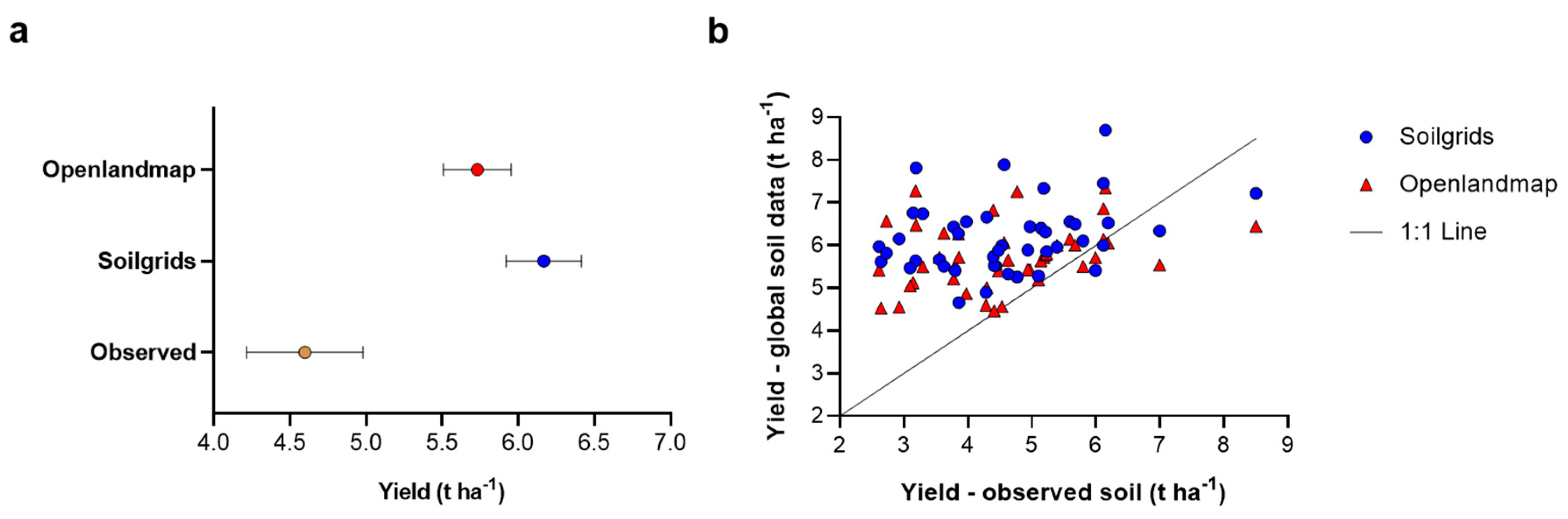
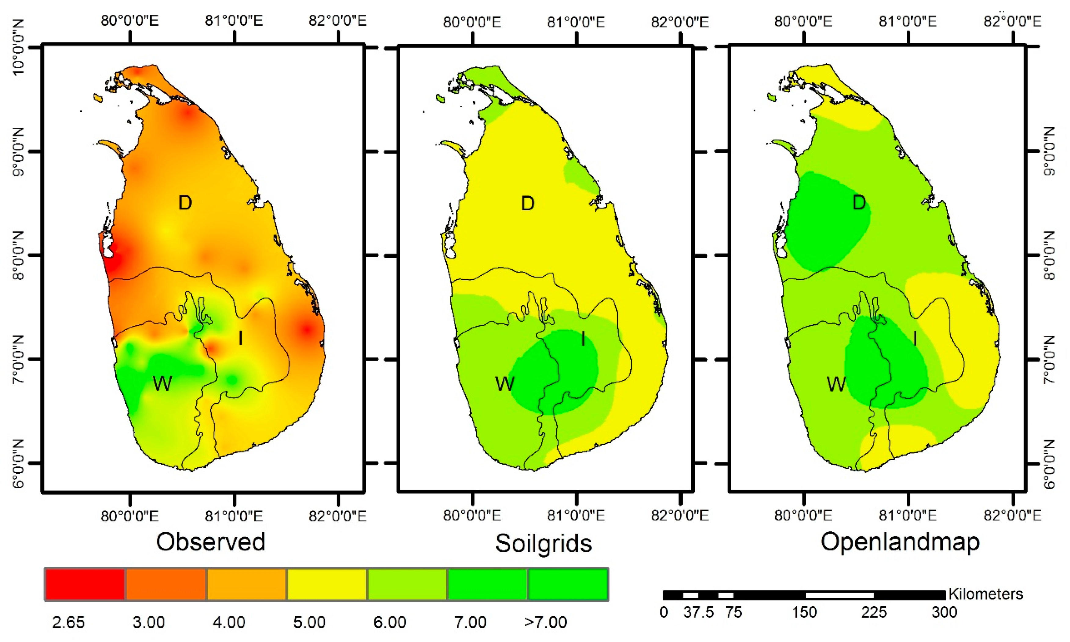
3.2. Simulated Rice Yield

The average simulated rice yield for observed soils was 4.60 ± 1.26 t ha⁻¹. Out of the three datasets, the highest (average) simulated rice yield was recorded with Soilgrids (6.17 ± 0.82 t ha⁻¹), followed by Openlandmap data (5.73 ± 0.74 t ha⁻¹). Rice yields simulated using both Soilgrids and Openlandmap soil data were significantly (p < 0.05) higher than the observed soil (Figure 6). However, the yields from two global soil databases were also significantly (p < 0.05) different from each other. A comparatively higher coefficient of variation (CV) was reported from observed soil (0.2735) than from Soilgrids (0.1322) and Openlandmap (0.1283) data.

Comparatively higher agreement (d = 0.27) with lower RMSE (1.69 t ha⁻¹) was reported for Openlandmap soils than for Soilgrids (

Table 2. Performance evaluation of the APSIM simulated yield from different soil databases.

Parameter	Observed vs. Soilgrids	Observed vs. Openlandmap	Soilgrids vs. Openlandmap
RMSE (t ha−1)	2.02	1.69	1.00
NRMSE	0.44	0.37	0.16
d	0.23	0.27	0.43

). However, the index of agreement was less than 0.3 indicating a poor agreement of yield between observed and global soil data. The RMSE between observed and Soilgrids yield was 2.02 t ha⁻¹. In contrast, a relatively higher agreement (d = 0.43) was observed between the yields from Soilgrids and Openlandmap soils. Out of all, 9.1% and 11.4% of the fields simulated using observed soil showed a higher yield than Soilgrids and Openalandmap, respectively. The slope of the regression curve in the Soilgrids simulated yield showed a significant (p < 0.05) deviation from zero while Openlandmap was not significant (p > 0.05) when compared with yield simulated using observed soil. The slopes of the regression lines were 0.1933 and 0.1672, respectively. Relatively higher correlation was reported from Soilgrids (r = 0.2982) than Openlandmap (r = 2860). Relatively higher agreement (r = 0.3209), which is significant (p < 0.05), was reported between Soilgrids and Openlandmap simulated yields.

Out of the three climatic zones, the highest observed yield was reported from the wet zone (5.54 t ha⁻¹) followed by the intermediate (4.81 t ha⁻¹) and dry zones (3.68 t ha⁻¹). The yields from Openlandmap showed the same pattern, however, the highest yield from Soilgrids soil was from the intermediate zone. The second highest yield from Soilgrids was from the wet zone. Out of the three climatic zones, the highest agreement of global data with observed yield was from the wet zone followed by the intermediate zone. The yield distribution pattern across the country was different according to soil databases (Figure 7). The highest yield from observed soil is from the southwestern part of the country (wet zone). The variability of yield from all three databases is due to spatial variation of both soil and climate.

The probability exceedance distribution of yield showed different patterns and did not separate according to the median values in all three soil datasets (Figure S2). Parallel to the mean yields, the highest yield at 0.5 probability exceedance level was observed from Soilgrids followed by Openlandmap and observed soil.

In Sri Lanka, nation-wide yield information for rice varieties is not available. However, the average rice yield for the major growing season in Sri Lanka during the 1980–2009 period was 3.70 ± 0.37 t ha⁻¹ (DOASL) and nearly consistent with the yield simulated using observed soil. It should be noted that observed yields are subject to different biotic and abiotic stresses such as pest and diseases, nutrient deficiencies and agroclimatic variability, whereas the simulations assume that these stresses are absent.

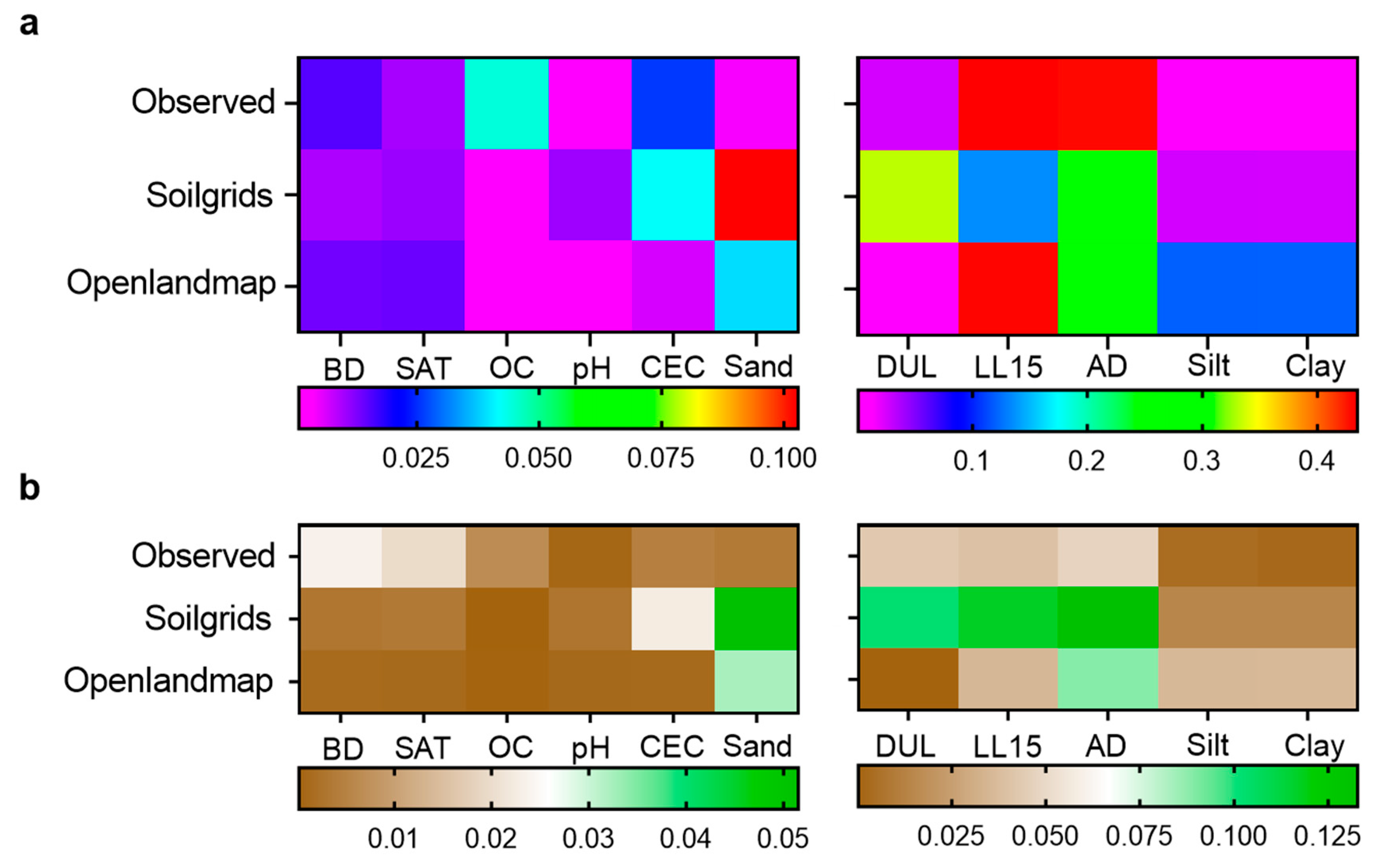
3.3. Sensitivity of Rice Yield to Soil Parameters

To ascertain the degree of sensitivity of yield to different parameters across the three soil datasets, a sensitivity analysis was carried out. The accuracy of each emulator in sensitivity tests was initially evaluated using the sigma squared value. The average sigma squared value over 30 years in observed soil was 0.123 which indicates a good linear relationship between the response and predictors. Comparatively lower sigma squared values were reported for global data (0.066 and 0.071 for Soilgrids and Openlandmap, respectively), suggesting a better linear relationship between predicted yield and soil parameters than observed data. The average R² value for the model fit was 0.99 in all the three data sets. The lower sigma squared and higher R² values indicate a good model fit for sensitivity analysis in all datasets; therefore, the models were used to study the sensitivity of input parameters.

The Shapley’s sensitivity index of 11 input parameters for three data sets is shown in Figure 8. According to the Shapley effect, LL15 is the most influential soil parameter followed by AD for APSIM simulated rice yield in both observed and Openlandmap datasets. However, DUL ranked as the most influential parameter in Soilgrids, followed by AD and LL15. In general, soil hydrological parameters have the highest impact on rice yield. The Shapley effect of none of the parameters in both observed and Soilgrids exceeded 0.1. In contrast, comparatively higher sensitivity was reported for silt and clay (Shapley effect 0.12) in Openlandmap data. It should be noted that DUL in Openlandmap and both LL15 and DUL in Soilgrids were derived from pedotransfer functions. All other parameters, BD, SAT, pH, OC, CEC and sand, were identified as less sensitive soil parameters for rice yield.

Of all parameters, the Shapley effect of soil bulk density and saturation (derived from BD) were not significantly different (p > 0.05) among datasets, while all other parameters were significantly (p < 0.05) different. Since DUL and LL15 were derived from soil texture, the choice of accurate texture data has a direct influence on the crop yield. Therefore, sand, silt and clay content from both Soilgrids and Openlandmap data were not suitable for yield simulations in the study area. However, due to low sensitivity and no significant difference (p > 0.05) between datasets, bulk density from global databases can still be used in crop models for yield simulations. Due to lower sensitivity, pH, OC, CEC can be obtained from global soil databases for yield simulations even though the values of some of them are significantly different from observed soil data.

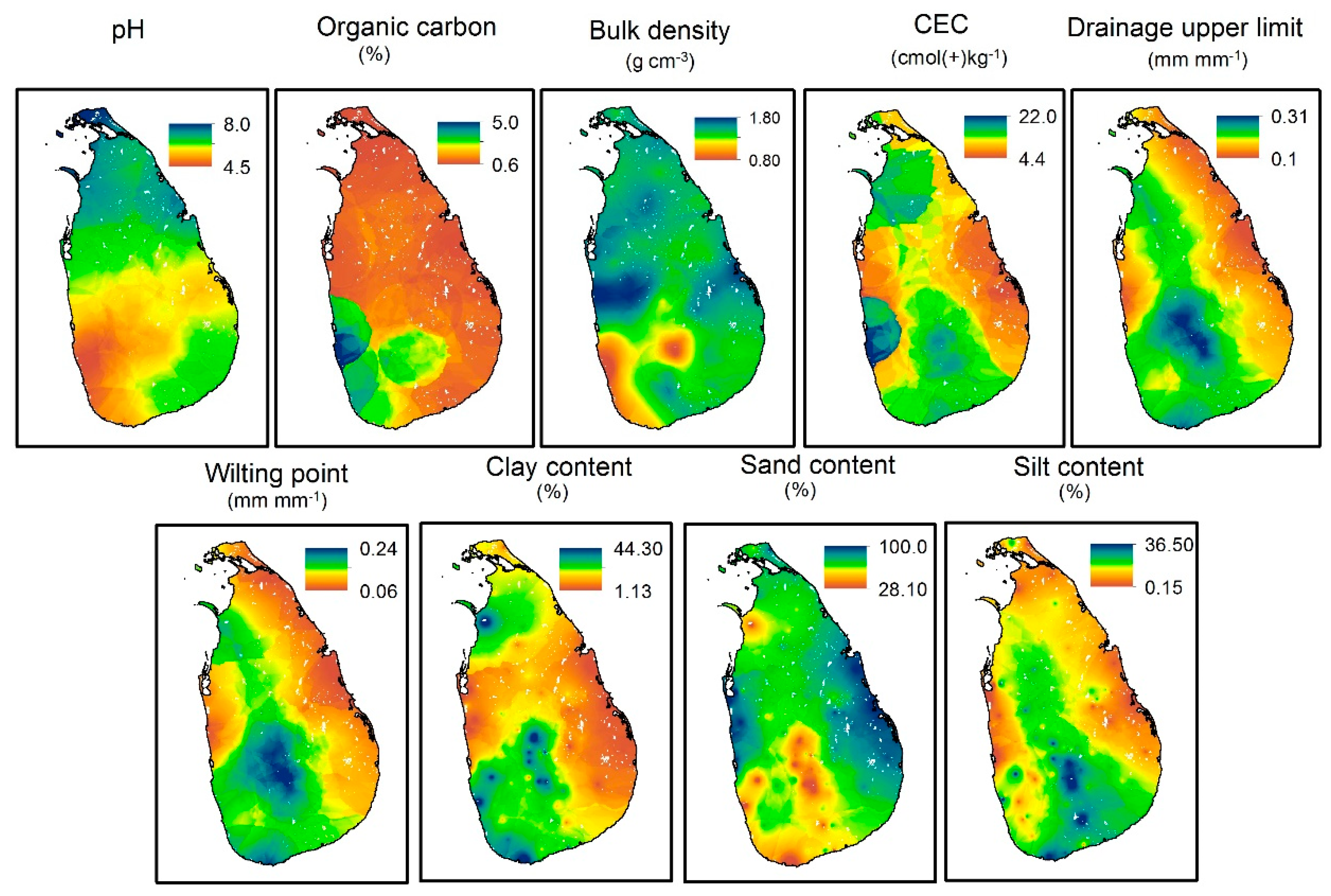
3.4. Interpolated Maps

Figure 9 shows an example of interpolated maps that were produced using a Bayesian kriging method. In general, pH patterns resemble the climate zones of Sri Lanka depicted in Figure 1. The prediction error map (available at http://dx.doi.org/10.17632/5sc7njfcyn.1) showed relatively higher standard error in coastal regions due to the lower density of sampling in those areas. The level of error remained constant in all soil layers and that indicates a good model fit. The same patterns can be seen with hydrological parameters as a distinction between climate zones is also evident in those maps.

Of all 9 parameters, volumetric moisture content (15 bars level) showed the lowest RMSE across all layers while CEC showed higher RMSE (

Table A1. The prediction accuracy of interpolation methods for soil attributes at 0–5, 5–15, 15–30, 30–60 and 60–100 cm layers in Sri Lanka Soil Parameter.

	Geostatistics Methods	Neighbourhood Types	Semivariogram Types/Kernel Function/General Properties	RMSE
				0–5 cm	5–15 cm	15–30 cm	30–60 cm	60–100 cm
pH	EBK	Smooth Circular	Linear	0.770	0.756	0.848	1.273	1.500
OC	EBK	Standard Circular	Linear	2.649	2.620	2.616	2.185	1.651
BD	EBK	Standard Circular	Linear	0.184	0.274	0.281	0.390	0.668
CEC	EBK	Standard Circular	Linear	14.949	14.765	14.301	12.761	8.177
DUL	EBK	Standard Circular	Linear	0.090	0.086	0.077	0.088	0.115
LL15	EBK	Standard Circular	Linear	0.082	0.078	0.070	0.074	0.091
Clay	RBF	Standard	Completely Regularised Spline	10.838	10.694	11.678	13.377	14.735
Sand	RBF	Standard	Completely Regularised Spline	15.970	15.861	16.482	20.565	21.368
Silt	RBF	Standard	Completely Regularised Spline	8.159	8.151	8.688	8.717	8.685

Note: OC = Organic carbon, BD = Bulk density, CEC = Cation exchange capacity, DUL = Drainage upper limit (VMC33), LL15 = Wilting point (VMC1500), EBK = Empirical Bayesian Kriging and RBF = Radial Basis Function.

). In general, interpolating soil physical properties proved to be challenging as the lowest RMSE for all three parameters belong to the Radial Basis function method which is a deterministic interpolation technique using a regularised spline method which does not use the inherent autocorrelation that exists in soil properties.

4. Discussion

Legacy soil survey data will provide an initial understanding of the diversity of soils and integration, and harmonisation of these data across standard horizons and per soil property is the first step towards improving their utility for digital soil mapping and yield modelling [19,60]. The heterogenicity of different soil parameters across Sri Lanka and within soil series was previously described [26]. Being a tropical country with diverse climatic, topographic and biodiversity variation, a high spatial variability is reported for soil parameters in Sri Lanka [26] and is also reflected in wide ranges for observed data in Figure 2 and Figure 3. The diversity of observed soil types is captured by global databases to some extent as some of the parameters such as pH in dry and wet zones in all three databases are significantly different. Rathnayake et al. [61] reported pH ranges of 4.1 to 7.7 (1:5) and >4.1 to 5.09 (1:5), respectively, in their study areas in DZ and WZ. Although all of the datasets used in this study show ranges within the range mentioned above, failure of observed data to reflect lower pH variation in DZ shows that more local data are required before any conclusion can be made regarding soil acidity in DZ as pH value is highly sensitive to soil moisture content.

Soilgrids was previously compared with observed data in Sri Lanka. Vitharana et al. [62] reported that soil organic carbon content stock in Sri Lanka reported by Soilgrids was overestimated by 122% in the 0–30 cm layer and 209% in the 30–100 cm layer than observed values. The average overestimation of organic carbon from Soilgrids and Openalandmap for all six depths (up to 200 cm) were 506% and 320% respectively, and higher than the amount reported by Vitharana et al. [62]. The higher discrepancy of organic carbon between observed and global data may be associated with elevation, slope angle and elevation, which were identified as major environmental controllers that determine spatial distribution of OC stocks [62].

The variation of soil properties in Sri Lanka is high as six out of twelve global taxonomic orders are found in the country [26]. This is reflected in the observed soil physical properties (sand %, silt % and clay %). This consistent underestimation of sand % and overestimation of silt % and clay % could be due to the standardisation filter that was applied to global datasets to make sure the total percentage of all three variables amounted to 100% [18].

As a consequence of this disparity, the pedotransfer functions (Equations (3)–(5) and (6)) are also affected. The inputs to calculate soil hydrological parameters using different pedotransfer functions are different [63]. Furthermore, pedotransfer function-derived soil hydrological parameters show significant difference among each other [63,64]. The impact of different pedotransfer functions on soil hydrological properties was not compared in this study, therefore, the choice of pedotransfer functions may also have an impact on the yield in two global databases.

Yields that were simulated using the global soil data were significantly (p < 0.05) higher than those of observed data. Therefore, the likely productivity of a certain crops cannot be determined by solely using the present version of global data. Although using global datasets is generally useful for providing an overview, their use in developing any understanding of crop performance at a local scale is questionable. However, as described in Section 3.3, these data can prove useful in filling the gaps in data, particularly for mapping the crop yield at the regional or national scales.

There is no threshold value to explain linearity or nonlinearity of developed models to study the sensitivity of inputs [44]. However, the increment of sigma squared value from 0.13 to 1.6 changed the linearity of the emulator to moderate nonlinearity [65]. The average sigma squared values for sensitivity analysis are within the acceptable range reported by Gunaratne et al. [44] suggesting a strong linear relationship between the log-transformed response and predictors for all models. Therefore, the sensitivity of fitted models in Shapley’s sensitivity analysis were accurate and able to capture the sensitivity of all tested inputs. Using GEM-SA software for sensitivity analysis, Gunarathna et al. [44] studied the sensitivity of soil input parameters into rice yield in Sri Lanka. Authors reported that the highest sensitivity for rice was for DUL followed by LL15. However, they did not include AD, which showed the highest sensitivity in the current study. Without AD, the sensitivity of inputs of the current study were consistent with the finding of Gunarathna et al. [44].

Soilgrids and Openlandmap used more than 100,000 field observations (derived from WoSIS and USDA databases) to develop the global datasets. However, only nine locations in Sri Lanka were reportedly used to provide property maps for Sri Lanka [19]. Perhaps, this is the reason for the low performance of models used to generate Soigrids data as only the pH model could explain more than 80% of variation [18]. This shows the importance of developing and validating local soil property datasets using locally harmonised survey information. The accuracy of global datasets will be greatly improved if the local soil datasets are openly accessible.

Different attempts have been made to map soil properties in different geographic scales using different techniques [66]. However, less attention is given to national level digital soil mapping that could benefit different end-users. One of the reasons for the lack of such attempts is the variation in units, property scales, depths, number of samples, and complexity of techniques. As shown by Ramcharan et al. [67] and Pásztor et al. [68], developing broad-scale soil property maps using low density of observation data (observation density up to 0.001 per km²) can still meet the need for soil simulation models. The utility of such data for crop modelling, however, should still be investigated. As the density of observed soil data increases, the amount of spatial autocorrelation resulting from similarity of soil samples will be improved. This will improve the results of interpolations used at the national level.

The importance of developing a web-based national soil database that could be readily available was highlighted by Mapa [66]. As a step toward filling the gap in national level digital soil database, we developed a digital 3D soil database that includes 9 parameters up to 100 cm depth. The accuracy of some of the maps that were produced is lower for CEC and soil physical properties (Figure 9). This is due to very low density of soil profile data across the country that leads to low amounts of spatial autocorrelation needed for successful interpolation. However, since the interpolated maps are produced using observed data, they can still be useful in ascertaining spatial variability of soil properties across Sri Lanka.

Soil data from two detailed and comprehensive datasets were used in the interpolations. Undoubtedly, there are several field observations in different parts of the country that were not used in mapping that could be used to improve predictions and create more accurate maps with other parameters. As the next step, we expect to collect more samples through a crowd-sourcing approach [69] using observation data and develop freely accessible detailed digital soil maps for Sri Lanka.

In this article, the impact of soil properties on one of the major crops was studied as a proxy. With the increased popularity of fewer-parameter crop models such as SIMPLE [70] in simulating underutilised crops that contributes to agricultural diversification [6,24], the findings of this article can be used. This is because, due to the dependency of low inputs, the choice of the correct soil database can severely affect the final yield estimations. Additionally, the method we followed to develop a country-specific soil database can be applied in locations where observed soil data are scarce for regional-level crop modelling that will in turn help with inclusion of other options in regional development programs.

5. Conclusions

Due to the unavailability of fine-scale harmonised observed soil data, relying on available big environmental data for yield simulation and mapping is the only option. In particular, modelling for underutilised crops, as a prerequisite for adoption of these crops into the crop diversification projects can greatly benefit from this data. To examine the applicability of open access soil data for crop modelling as a primer for further calibration models for minor crops, we compared the results of models using three databases. Using an exemplar crop model (APSIM), we found that the majority of global soil data are not a good option to fill gaps due to the significant deviations with observed data, however, they might still be used for yield simulation. The APSIM simulated yields for global soil data were significantly different from those of observed soil. Soil hydrological parameters such as LL15 (wilting point), AD (soil moisture limit to which soil can dry by evaporation) and DUL (drainage upper limit) were identified as the most sensitive inputs for simulated rice yield. Due to the comparatively lower sensitivity to yield, other soil parameters such as pH, CEC and organic carbon from global databases can be used in APSIM modelling where observed data are not available. However, bulk density and textural properties from global databases should be used with caution as they influence the soil hydrological parameters using pedotransfer functions. Newly developed digital soil maps that contain nine soil properties up to 100 cm depth are freely available and can be used as an alternative to global soil databases in cases when local data are not available. To allow for wider accessibility, the data were stored in a free repository (doi:10.17632/5sc7njfcyn.1) that can be accessed by anyone who is interested.

References

1. Karunaratne, A.S.; Walker, S.; Ruane, A.C. Modelling Bambara groundnut yield in Southern Africa: Towards a climate-resilient future. Clim. Res. 2015, 65, 193–203. [Google Scholar] [CrossRef]
2. Holzworth, D.P.; Huth, N.I.; deVoil, P.G.; Zurcher, E.J.; Herrmann, N.I.; McLean, G.; Chenu, K.; van Oosterom, E.J.; Snow, V.; Murphy, C.; et al. APSIM—Evolution towards a new generation of agricultural systems simulation. Environ. Model. Softw. 2014, 62, 327–350. [Google Scholar] [CrossRef]
3. Chisanga, C.B.; Phiri, E.; Chinene, V.R.N. Climate change impact on maize (Zea mays L.) yield using crop simulation and statistical downscaling models: A review. Sci. Res. Essays 2017, 12, 167–187. [Google Scholar] [CrossRef] [Green Version]
4. Madegwa, Y.M. Modelling Nutrient Dynamics and Yield of Finger Millet (Eleusine Coracana) in Semi-Arid Eastern Kenya, Using the Agricultural Production Systems Simulator Model (APSIM). Master’s Thesis, University of Nairobi, Nairobi, Kenya, 2015. [Google Scholar]
5. Li, X.; Zhu, C.; Wang, J.; Yu, J. Chapter six—Computer Simulation in Plant Breeding. In Advances in Agronomy; Sparks, D.L., Ed.; Academic Press: Cambridge, MA, USA, 2012; Volume 116, pp. 219–264. [Google Scholar]
6. Jahanshiri, E.; Mohd Nizar, N.M.; Tengku Mohd Suhairi, T.A.S.; Gregory, P.J.; Mohamed, A.S.; Wimalasiri, E.M.; Azam-Ali, S.N. A Land Evaluation Framework for Agricultural Diversification. Sustainability 2020, 12, 3110. [Google Scholar] [CrossRef] [Green Version]
7. Mabhaudhi, T.; Modi, A.T.; Beletse, Y.G. Parameterisation and evaluation of the FAO-AquaCrop model for a South African taro (Colocasia esculenta L. Schott) landrace. Agric. For. Meteorol. 2014, 192, 132–139. [Google Scholar] [CrossRef]
8. Sharda, V.; Handyside, C.; Chaves, B.; McNider, R.T.; Hoogenboom, G. The impact of spatial soil variability on simulation of regional maize yield. Trans. Asabe 2017, 60, 2137–2148. [Google Scholar] [CrossRef]
9. Folberth, C.; Skalský, R.; Moltchanova, E.; Balkovič, J.; Azevedo, L.B.; Obersteiner, M.; van der Velde, M. Uncertainty in soil data can outweigh climate impact signals in global crop yield simulations. Nat. Commun. 2016, 7, 11872. [Google Scholar] [CrossRef] [Green Version]
10. Woli, P.; Paz, J.O.; Hoogenboom, G.; Garcia y Garcia, A.; Fraisse, C.W. The ENSO effect on peanut yield as influenced by planting date and soil type. Agric. Syst. 2013, 121, 1–8. [Google Scholar] [CrossRef]
11. Kuleshov, Y. Use of Remote Sensing Data for Climate Monitoring in WMO Regions II and V (Asia and the South-West Pacific); World Meteorological Organization: Geneva, Switzerland, 2017. [Google Scholar]
12. Han, E.; Ines, A.V.M.; Koo, J. Development of a 10-km resolution global soil profile dataset for crop modeling applications. Environ. Model. Softw. 2019, 119, 70–83. [Google Scholar] [CrossRef]
13. Hengl, T.; MacMillan, R.A. Predictive Soil Mapping with R; OpenGeoHub foundation: Wageningen, The Netherlands, 2019; ISBN 978-0-359-30635-0. [Google Scholar]
14. Nachtergaele, F.; van Velthuizen, H.; Verelst, L.; Batjes, N.; Dijkshoorn, K.; van Engelen, V.; Fischer, G.; Jones, A.; Montanarella, L.; Petri, M.; et al. Harmonized World Soil Database; Food and Agriculture Organization of the United Nations: Rome, Italy, 2009. [Google Scholar]
15. Batjes, N. ISRIC-WISE Derived Soil Properties on a 5 by 5 Arc-Minutes Global Grid (Ver. 1.2); ISRIC: Wageningen, The Netherlands, 2012; p. 56. [Google Scholar]
16. Ribeiro, E.; Batjes, N.H.; van Oostrum, A.J.M. World Soil Information Service (WoSIS)—Towards the Standardization and Harmonization of World Soil Data; ISRIC—World Soil Information: Wageningen, The Netherlands, 2018; p. 151. [Google Scholar]
17. Batjes, N.H.; Ribeiro, E.; van Oostrum, A. Standardised soil profile data to support global mapping and modelling (WoSIS snapshot 2019). Earth Syst. Sci. Data 2020, 12, 299–320. [Google Scholar] [CrossRef] [Green Version]
18. Hengl, T.; de Jesus, J.M.; Heuvelink, G.B.M.; Gonzalez, M.R.; Kilibarda, M.; Blagotić, A.; Shangguan, W.; Wright, M.N.; Geng, X.; Bauer-Marschallinger, B.; et al. SoilGrids250m: Global gridded soil information based on machine learning. PLoS ONE 2017, 12, e0169748. [Google Scholar] [CrossRef] [PubMed] [Green Version]
19. Hengl, T.; Collins, T.N.; Wheeler, I.; MacMillan, R.A. Everybody Has a Right to Know What’s Happening with the Planet: Towards a Global Commons. Available online: http://doi.org/10.5281/zenodo.3274294 (accessed on 21 September 2020).
20. Kim, K.S.; Yoo, B.H.; Shelia, V.; Porter, C.H.; Hoogenboom, G. START: A data preparation tool for crop simulation models using web-based soil databases. Comput. Electron. Agric. 2018, 154, 256–264. [Google Scholar] [CrossRef]
21. Jones, J.W.; Hoogenboom, G.; Porter, C.H.; Boote, K.J.; Batchelor, W.D.; Hunt, L.A.; Wilkens, P.W.; Singh, U.; Gijsman, A.J.; Ritchie, J.T. The DSSAT cropping system model. Eur. J. Agron. 2003, 18, 235–265. [Google Scholar] [CrossRef]
22. Varella, H.; Guérif, M.; Buis, S. Global sensitivity analysis measures the quality of parameter estimation: The case of soil parameters and a crop model. Environ. Model. Softw. 2010, 25, 310–319. [Google Scholar] [CrossRef]
23. Vanuytrecht, E.; Raes, D.; Willems, P. Global sensitivity analysis of yield output from the water productivity model. Environ. Model. Softw. 2014, 51, 323–332. [Google Scholar] [CrossRef] [Green Version]
24. Manna, P.; Bonfante, A.; Perego, A.; Acutis, M.; Jahanshiri, E.; Ali, S.A.; Basile, A.; Terribile, F. LANDSUPPORT DSS Approach for Crop Adaptation Evaluation to the Combined Effect of Climate Change and Soil Spatial Variability. Geophys. Res. Abstr. 2019, 21, 15457. [Google Scholar]
25. Punyawardena, B.V.R. Precipitation of Sri Lanka and Agro-Ecological Regions; Agriculture Press: Peradeniya, Sri Lanka, 2008. [Google Scholar]
26. Mapa, R.B. Soil research and soil mapping history. In The Soils of Sri Lanka; Mapa, R.B., Ed.; Springer Nature: Cham, Switzerland, 2020; pp. 1–11. [Google Scholar]
27. Mapa, R.B.; Somasiri, S.; Magarajah, S. Soils of the Wet Zone of Sri Lanka: Morphology, Characterization and Classification: Special Publication No. 1; Soil Science Society of Sri Lanka, Sarvodaya Wishva Lekha: Colombo, Sri Lanka, 1999. [Google Scholar]
28. Mapa, R.B.; Dassanayake, A.R.; Nayakekorale, H.B. Soils of the Intermediate Zone of Sri Lanka: Morphology, Characterization and Classification. Special Publication No. 4; Soil Science Society of Sri Lanka, Sarvodaya Wishva Lekha: Colombo, Sri Lanka, 2005. [Google Scholar]
29. Mapa, R.B.; Somasiri, S.; Dassanayake, A.R. Soils of the Dry Zone of Sri Lanka: Morphology, Characterization and Classification. Special Publication No. 7; Soil Science Society of Sri Lanka, Sarvodaya Wishva Lekha: Colombo, Sri Lanka, 2010. [Google Scholar]
30. Mapa, R.B. Characterization of Soils in the Northern Region of Sri Lanka to Develop a Soil Data Base for Land Use Planning and Environmental Applications; National Research Council of Sri Lanka: Colombo, Sri Lanka, 2016. [Google Scholar]
31. Kabała, C.; Musztyfaga, E.; Gałka, B.; Łabuńska, D.; Mańczyńska, P. Conversion of Soil pH 1:2.5 KCl and 1:2.5 H2O to 1:5 H2O: Conclusions for Soil Management, Environmental Monitoring, and International Soil Databases. Pol. J. Environ. Stud. 2016, 25, 647–653. [Google Scholar] [CrossRef]
32. Libohova, Z.; Wills, S.; Odgers, N.P.; Ferguson, R.; Nesser, R.; Thompson, J.A.; West, L.T.; Hempel, J.W. Converting pH1:1 H2O and 1:2CaCl2 to 1:5 H2O to contribute to a harmonized global soil database. Geoderma 2014, 213, 544–550. [Google Scholar] [CrossRef]
33. Gunarathna, M.H.J.P.; Sakai, K.; Nakandakari, T.; Momii, K.; Kumari, M.K.N.; Amarasekara, M.G.T.S. Pedotransfer functions to estimate hydraulic properties of tropical Sri Lankan soils. Soil Till. Res. 2019, 190, 109–119. [Google Scholar] [CrossRef]
34. Dalgliesh, N.; Hochman, Z.; Huth, N.; Holzworth, D. Field Protocol to APSoil Characterisations. Version 4; CSIRO: Black Mountain, Australia, 2016. [Google Scholar]
35. Bishop, T.F.A.; McBratney, A.B.; Laslett, G.M. Modelling soil attribute depth functions with equal-area quadratic smoothing splines. Geoderma 1999, 91, 27–45. [Google Scholar] [CrossRef]
36. Agstat—Agricultural Statistics; Socio Economics and Planning Centre, Department of Agriculture: Peradeniya, Sri Lanka, 2019.
37. Keating, B.A.; Carberry, P.S.; Hammer, G.L.; Probert, M.E.; Robertson, M.J.; Holzworth, D.; Huth, N.I.; Hargreaves, J.N.G.; Meinke, H.; Hochman, Z.; et al. An overview of APSIM, a model designed for farming systems simulation. Eur. J. Agron. 2003, 18, 267–288. [Google Scholar] [CrossRef] [Green Version]
38. Gaydon, D.S.; Probert, M.E.; Buresh, R.J.; Meinke, H.; Suriadi, A.; Dobermann, A.; Bouman, B.; Timsina, J. Rice in cropping systems—Modelling transitions between flooded and non-flooded soil environments. Eur. J. Agron. 2012, 39, 9–24. [Google Scholar] [CrossRef]
39. Probert, M.E.; Dimes, J.P.; Keating, B.A.; Dalal, R.C.; Strong, W.M. APSIM’s water and nitrogen modules and simulation of the dynamics of water and nitrogen in fallow systems. Agric. Syst. 1998, 56, 1–28. [Google Scholar] [CrossRef]
40. Zubair, L.; Nissanka, S.P.; Weerakoon, W.M.W.; Herath, D.I.; Karunaratne, A.S.; Prabodha, A.S.M.; Agalawatte, M.B.; Herath, R.M.; Yahiya, S.Z.; Punyawardhene, B.V.R.; et al. Climate Change Impacts on Rice Farming Systems in Northwestern Sri Lanka. In Series on Climate Change Impacts, Adaptation, and Mitigation; Imperial College Press: London, UK, 2015; Volume 4, pp. 315–352. ISBN 978-1-78326-563-3. [Google Scholar]
41. Ruane, A.C.; Goldberg, R.; Chryssanthacopoulos, J. Climate forcing datasets for agricultural modeling: Merged products for gap-filling and historical climate series estimation. Agric. For. Meteorol. 2015, 200, 233–248. [Google Scholar] [CrossRef] [Green Version]
42. Lashkari, A.; Salehnia, N.; Asadi, S.; Paymard, P.; Zare, H.; Bannayan, M. Evaluation of different gridded rainfall datasets for rainfed wheat yield prediction in an arid environment. Int. J. Biometeorol. 2018, 62, 1543–1556. [Google Scholar] [CrossRef]
43. Ceglar, A.; Toreti, A.; Balsamo, G.; Kobayashi, S. Precipitation over Monsoon Asia: A Comparison of Reanalyses and Observations. J. Clim. 2017, 30, 465–476. [Google Scholar] [CrossRef]
44. Gunarathna, M.H.J.P.; Sakai, K.; Kumari, M.K.N.; Ranagalage, M. A Functional Analysis of Pedotransfer Functions Developed for Sri Lankan soils: Applicability for Process-Based Crop Models. Agronomy 2020, 10, 285. [Google Scholar] [CrossRef] [Green Version]
45. Sobol, I.M. Sensitivity estimates for nonlinear mathematical models. Math. Modeling Comput. Exp. 1993, 4, 407–414. [Google Scholar]
46. Owen, G. Game Theory; Academic Press: New York, NY, USA, 1982. [Google Scholar]
47. Roth, A.E. The Shapley Value as a von Neumann-Morgenstern Utility. Econometrica 1977, 45, 657–664. [Google Scholar] [CrossRef]
48. Roth, A.E. The Shapley Value: Essays in Honor of Lloyd S. Shapley; Cambridge University Press: Cambridge, UK, 1988. [Google Scholar]
49. Gong, X. Towards Understanding Crop Yield Systemic Risk and Its Implication for Crop Insurance Choices. Master’s Thesis, Michigan State University, Ann Arbor, MI, USA, 2019. [Google Scholar]
50. Lipovetsky, S.; Conklin, M. Analysis of regression in game theory approach. Appl. Stoch. Model. Bus. 2001, 17, 319–330. [Google Scholar] [CrossRef]
51. Owen, A.B.; Prieur, C. On Shapley Value for Measuring Importance of Dependent Inputs. Siam-Asa J. Uncertain. 2017, 5, 986–1002. [Google Scholar] [CrossRef] [Green Version]
52. R Core Team. R: A Language and Environment for Statistical Computing; R Foundation for Statistical Computing: Vienna, Austria, 2013. [Google Scholar]
53. Broto, B.; Bachoc, F.; Depecker, M.; Martinez, J.M. Sensitivity indices for independent groups of variables. Math. Comput. Simul. 2019, 163, 19–31. [Google Scholar] [CrossRef] [Green Version]
54. Shapiro, S.S.; Wilk, M.B. An Analysis of Variance Test for Normality (Complete Samples). Biometrika 1965, 52, 591–611. [Google Scholar] [CrossRef]
55. Royston, J.P. An Extension of Shapiro and Wilk’s W Test for Normality to Large Samples. J. R. Stat. Soc. C Appl. 1982, 31, 115–124. [Google Scholar] [CrossRef]
56. Ahmed, H.; Siddique, M.T.; Iqbal, M.; Hussain, F. Comparative study of interpolation methods for mapping soil pH in the apple orchards of Murree, Pakistan. Soil Environ. 2017, 36, 70–76. [Google Scholar] [CrossRef]
57. Li, J.; Heap, A.D. A review of comparative studies of spatial interpolation methods in environmental sciences: Performance and impact factors. Ecol. Inform. 2011, 6, 228–241. [Google Scholar] [CrossRef]
58. Yasrebi, J.; Saffari, M.; Fathi, H.; Karimian, N.; Moazallahi, M.; Gazni, R. Evaluation and comparison of Ordinary Kriging and Inverse Distance Weighting methods for prediction of spatial variability of some soil chemical parameters. Res. J. Biol. Sci. 2009, 4, 93–102. [Google Scholar]
59. Rodrigues, M.S.; Alves, D.C.; de Souza, V.C.; de Melo, A.C.; Lima, A.M.N.; Cunha, J.C. Spatial interpolation techniques for site-specific irrigation management in a mango orchard. Comun. Sci. 2018, 9, 93–101. [Google Scholar] [CrossRef]
60. Sulaeman, Y.; Minasny, B.; McBratney, A.B.; Sarwani, M.; Sutandi, A. Harmonizing legacy soil data for digital soil mapping in Indonesia. Geoderma 2013, 192, 77–85. [Google Scholar] [CrossRef]
61. Rathnayake, W.M.U.K.; De Silva, R.P.; Dayawansa, N.D.K. Variability of some important soil chemical properties of rainfed low land paddy fields and its effect on land suitability for rice cultivation. Trop. Agric. Res. 2015, 26, 506. [Google Scholar] [CrossRef]
62. Vitharana, U.W.A.; Mishra, U.; Mapa, R.B. National soil organic carbon estimates can improve global estimates. Geoderma 2019, 337, 55–64. [Google Scholar] [CrossRef]
63. Botula, Y.D.; Cornelis, W.M.; Baert, G.; Van Ranst, E. Evaluation of pedotransfer functions for predicting water retention of soils in Lower Congo (D.R. Congo). Agric. Water Manag. 2012, 111, 1–10. [Google Scholar] [CrossRef]
64. Ryczek, M.; Kruk, E.; Malec, M.; Klatka, S. Comparison of pedotransfer functions for the determination of saturated hydraulic conductivity coefficient. Environ. Prot. Nat. Resour. 2017, 28, 25–30. [Google Scholar] [CrossRef] [Green Version]
65. Petropoulos, G.; Wooster, M.J.; Carlson, T.N.; Kennedy, M.C.; Scholze, M. A global Bayesian sensitivity analysis of the 1d SimSphere soil–vegetation–atmospheric transfer (SVAT) model using Gaussian model emulation. Ecol. Model. 2009, 220, 2427–2440. [Google Scholar] [CrossRef]
66. Vitharana, U.W.A.; Mapa, R.B. Soil survey, classification and mapping in Sri Lanka: Past, present and future. In Agricultural Research for Sustainable Food Systems in Sri Lanka; Marambe, B., Weerahewa, J., Dandeniya, W.S., Eds.; Springer Nature: Singapore, 2020; Volume 1, pp. 77–100. [Google Scholar]
67. Ramcharan, A.; Hengl, T.; Nauman, T.; Brungard, C.; Waltman, S.; Wills, S.; Thompson, J. Soil Property and Class Maps of the Conterminous United States at 100-Meter Spatial Resolution. Soil Sci. Soc. Am. J. 2018, 82, 186–201. [Google Scholar] [CrossRef] [Green Version]
68. Pásztor, L.; Laborczi, A.; Bakacsi, Z.; Szabó, J.; Illés, G. Compilation of a national soil-type map for Hungary by sequential classification methods. Geoderma 2018, 311, 93–108. [Google Scholar] [CrossRef] [Green Version]
69. Herrick, J.E.; Beh, A.; Barrios, E.; Bouvier, I.; Coetzee, M.; Dent, D.; Elias, E.; Hengl, T.; Karl, J.W.; Liniger, H.; et al. The land-potential knowledge system (landpks): Mobile apps and collaboration for optimizing climate change investments. Ecosyst. Health Sustain. 2016, 2, e01209. [Google Scholar] [CrossRef] [Green Version]
70. Zhao, C.; Liu, B.; Xiao, L.; Hoogenboom, G.; Boote, K.J.; Kassie, B.T.; Pavan, W.; Shelia, V.; Kim, K.S.; Hernandez-Ochoa, I.M.; et al. A SIMPLE crop model. Eur. J. Agron. 2019, 104, 97–106. [Google Scholar] [CrossRef]
Figure 1. A map of Sri Lanka showing the soil sample collection sites (triangles) and locations used for detailed comparison with global data and Agricultural Production Systems Simulator (APSIM) simulations (dots). Major climatic zones are marked based on the agroecological classification of Punyawardene [25].
Sustainability 12 07781 g001
Figure 2. Comparison of average (a) bulk density, (b) pH, (c) organic carbon, (d) sand, (e) silt and (f) clay content of all standard profiles in observed (OB), Soilgrids (SG) and Openlandmap (OLM) databases. The 95% confidence interval is shown in bars. WZ, IZ and DZ stand for wet zone, intermediate zone and dry zone, respectively.
Sustainability 12 07781 g002
Figure 3. Comparison of average (a) saturation, (b) drainage upper limit (DUL), (c) permanent wilting point (LL15), (d) Air Dry and (e) cation exchange capacity of all standard profiles in observed (OB), Soilgrids (SG) and Openlandmap (OLM) databases. The 95% confidence interval is shown in bars. WZ, IZ and DZ stand for wet zone, intermediate zone and dry zone, respectively.
Sustainability 12 07781 g003
Figure 4. Comparison of soil textural properties in (a) observed, (b) Soilgrids and (c) Openlandmap databases.
Sustainability 12 07781 g004
Figure 5. Comparison of the coefficient of variation in Soilgrids and Openlandmap databases with observed values in all the parameters in (a) dry zone, (b) intermediate zone and (c) wet zone.
Sustainability 12 07781 g005
Figure 6. (a) Average rice yield under different soils with 95% confidence interval and (b) 1:1 graph for yield simulated using observed, Soilgrids and Openlandmap data.
Sustainability 12 07781 g006
Figure 7. Comparison of interpolated APSIM simulated rice yields (t ha−1) from observed, Soilgrids and Openlandmap soil. Major climatic zones were marked as D = dry zone, I = intermediate zone and W = wet zone.
Sustainability 12 07781 g007
Figure 8. (a) Variation of the average Shapley index of selected soil properties on rice yield and (b) their standard deviations.
Sustainability 12 07781 g008
Figure 9. Interpolated soil properties in Sri Lanka for the 0–5 cm layer.
Sustainability 12 07781 g009