Article

Spatial Accessibility Analysis of Parks with Multiple Entrances Based on Real-Time Travel: The Case Study in Beijing

1
College of Resources Environment and Tourism, Capital Normal University, Beijing 100048, China
2
Beijing Laboratory of Water Resources Security, Capital Normal University, Beijing 100048, China
3
3D Information Collection and Application Key Lab of Education Ministry, Capital Normal University, Beijing 100048, China
4
Beijing State Key Laboratory Incubation Base of Urban Environmental Processes and Digital Simulation, Capital Normal University, Beijing 100048, China
5
College of Geography and Environment, Shandong Normal University, Jinan 250014, China
*
Author to whom correspondence should be addressed.
Sustainability 2020, 12(18), 7618; https://doi.org/10.3390/su12187618
Submission received: 14 August 2020 / Revised: 8 September 2020 / Accepted: 11 September 2020 / Published: 16 September 2020

Abstract

:
Parks are an important component of the green infrastructure in cities. They provide multiple benefits for residents’ life. Due to the uneven spatial distribution of parks, it is necessary to evaluate the spatial disparity about residents’ access to parks. The two-step floating catchment area method is suitable for measuring the accessibility of urban parks. However, few studies have noticed the representative of entrances of parks, especially adding them into the process of accessibility measurements. The floating catchment area is often determined by road speed and empirical travel time. In this article, the impact of multi-entrances of the park will be considered and real-time travel time is used in calculating accessibility. In a case of multi-entrance parks in Beijing, the average travel time of the sub-district is calculated, and with the support of the modified method, the spatial accessibilities of car driving, public transport and car-public transport mixed travel modes are obtained. The results show that the time–space compression effect of car driving is more obvious and the mixed travel mode presents the advantage of high accessibility index. This study has a theoretical and practical value for urban planning, such as advising urban planners on the siting of green park space.

1. Introduction

As an important element of urban green infrastructure, parks play a vital role in the construction of environmentally sustainable cities [1]. They are the link between human beings and the natural environment in urbanized areas, providing the urban residents with material, spiritual, economic and social benefits [2,3,4].
From the perspective of the environment, parks are known to protect urban biodiversity, provide urban ecosystem services and abundant landscape resources for cities [5]. In addition, urban land covered with vegetation can improve the air quality [6] and alleviate the urban heat island effect [7,8]. From the perspective of residents’ lives, urban parks offer convenient recreational and learning areas for residents. On the one hand, studies have shown that the presence of parks increases the opportunities for residents’ activities and communication with other people, which can enhance their health, both physical [9,10] and mental [11,12]. On the other hand, many parks are historical sites or are built with important activities. They are the most natural learning places for residents, especially teenagers. In addition, they also offer social and economic benefits through enhancing the economic vitality of the areas around them [13]. Considering these benefits, city managers and planners have stressed the necessity for adequate urban public green space [14]. However, with the rapid increase in residents’ demand for leisure and entertainment activities [15], many cities still face the problems of limited park resources [16] and the uneven spatial distribution of parks. As a consequence, in order to propose tailor-made interventions, researchers and urban planners have raised interest regarding how to identify the areas with potential risks for uneven distribution. Some scholars have investigated the disparity between the supply of urban green space and the demand of populations from the perspective of socio-economic status and demographic data [17,18], but their research results are far from reaching a consensus [19]. Therefore, concise and clear concepts and models are needed to measure the access. Through some studies and discussion, accessibility was considered to be available for evaluating access to public facilities such as parks. It can measure the ability of residents to access public parks and further reflect the rationality and fairness of the allocation of urban parks [20,21].
Accessibility refers to “the potential of opportunities for interaction” [22]. Although scholars have proposed different methods, such as cumulative models, gravity models, and proximity models [23,24,25], and have done a lot of research in the field of accessibility, such as Kong et al. in 2017 and Cheng et al. in 2019 [26,27], the essence of accessibility is the convenience level from one place to another via a certain transport system [28]. It is affected by the supply (starting points), the demand (destination points) and the spatial connection, which is usually measured by the travel cost, such as time and distance, between them [29]. First proposed by Radke and Mu [30] and then improved by Luo and Wang [31], the two-step floating catchment area (2SFCA) method is a special extension based on gravity models. It repeats twice when searching the floating catchment area, and can consider the supply, the potential demand and travel cost at the same time. Thus, it has been one of the most widely used methods in previous studies. In order to obtain better accessibility results, a series of improvements have been performed from 2SFCA. Luo and Qi proposed an enhanced 2SFCA that improves the actual simulation by dividing catchment into multiple zones based on multiple travel times [32]. The function of distance decay has also been introduced into 2SFCA to enhance it to get more precise results [33]. In reality, the supply-demand ratio is a continuous function, and thus the Gaussian function [34] and Kernel density function [35] was utilized.
The park is an important amenity in promoting urban residents’ quality of life. There are many empirical experiments about the accessibility to park study field. The spatial disparity of accessibility in cities has attracted the attention of scholars. In order to evaluate the spatial disparity between parks and the demanders, Li and Du et al. performed a modified a Gaussian-based 2SFCA method in Shenzhen [36]. They set out hierarchical systems with four types of distance. The results show that 40% of communities have a high population density but low accessibility of parks. A study paid attention to the accessibility of country parks between 14 country parks and 240 streets/towns in Shanghai [37]. The results show that most streets/towns have a low index value of the country parks, especially in the center area of Shanghai. A study using a long time series is helpful to find out the improvement degree of accessibility. A dynamic park accessibility analysis was undertaken of Hangzhou metropolitan area in China from 2016 to 2018 [38]. Based on this, researchers further proposed a machine learning algorithm to study the relationship between community deprivation and park accessibility changes. Wei evaluated the changes in accessibility over a decade in the 41 sub-districts of Hangzhou [39]. These studies can further supply information for analyzing the equality problem within the city. Some articles performed the research in the perspective of the vulnerable groups’ accessibility. Scholars added a new data source (mobile phone data) into 2SFCA when evaluating the access to urban park resources by the older people, as older people have limited physical mobility and the traditional census data lack some behavior-based information [40]. Xing et al. proposed a supply–demand improved 2SFCA method to estimate the spatial access to parks for youth in Wuhan [41]. The impact of data aggregation has also been noted. An E2SFCA method was utilized to measure and compare the spatial accessibility of the park at the micro and macro levels [42].
Nevertheless, there are some improvements in some aspects. First, the geometric centroids or centers of parks were regarded as the proxy for parks. However, in reality, many parks are gated and cannot be easily accessed at all points [39]. Residents can easily access those parks from the gates rather than the geometric centroids or centers of parks. Large or medium-sized parks (area more than 0.1 km 2 ) have multiple entrances, which will affect the estimated results of accessibility of parks, especially in urban parks, topic parks and district parks. Recently, some articles realized the effect of multiple entrances on the park’s service scope and used the entrances to calculate accessibility [41,43,44]. Nevertheless, they did not pay particular attention to the impact of the entrances on the entire service area of the park and on the attainable accessibility of demand points. In a word, up to now, the consideration of multi-entrances in the study of accessibility measures of urban parks is low. Moreover, researchers have mostly used the digital road network, combined with the empirical road speed and the empirical travel time to study the accessibility of parks. In fact, residents’ travel is a complex process. Only using empirical data can greatly simplify the process and may cause data errors. Furthermore, in terms of service capacity (also known as attraction coefficient) measurement, taking area as the only one measuring standard of service capacity may be improper. Having considered other factors [45], they are not widely used.
Overall, this study improved the accessibility measurement method for multiple-entrance urban parks as follow:
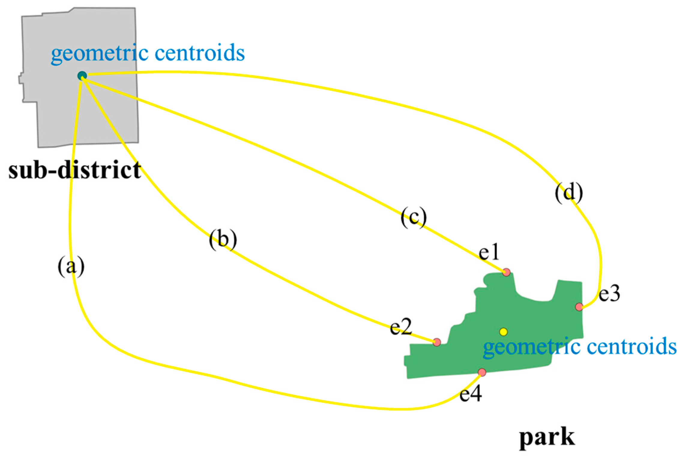
  • All entrances of parks are treated as the destinations and are specially calculated in the modified 2SFCA method.
  • The real-time travel time from Baidu Map is used to measure the cost between urban parks and residents.
  • The park grade as a parameter is added into the 2SFCA method, which is easy to obtain and is a sigh of the overall level of the park.
For better demonstrating our method, this article chooses large or medium-sized parks with multiple entrances in parks labelled for empirical experiments. The structure of this article is divided as follows: Section 2 briefly introduces the study area and data acquisition methods. Section 3 describes the research method used to measure accessibility. Section 4 evaluates the results of accessibility research. Section 5 is the discussion and Section 6 is the conclusion for this article.

2. Experimental Data and Study Area
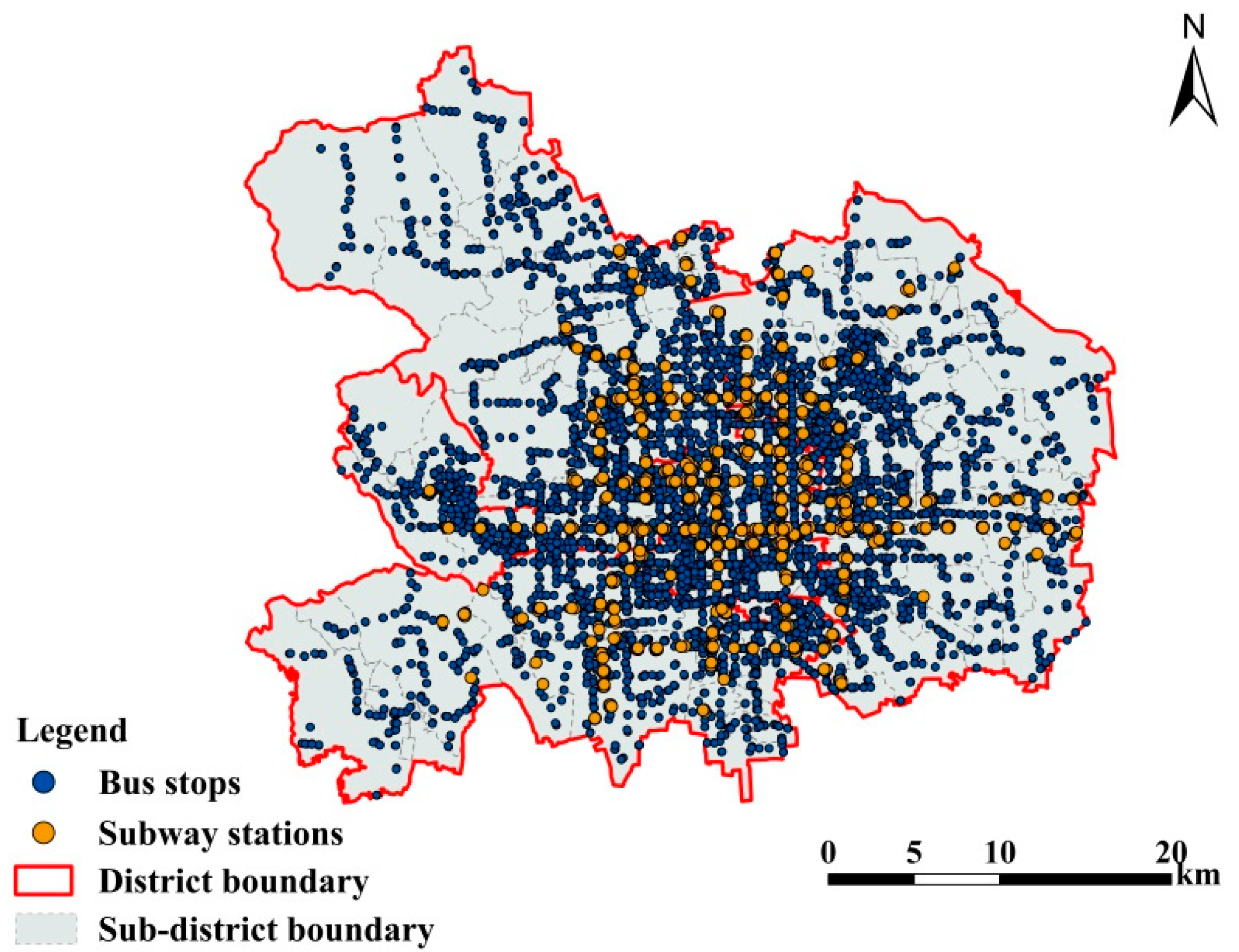
2.1. Study Area

Beijing is the capital city of China with a huge population. It is a national political, economic and cultural center, as well as a world-famous ancient capital and modern international city. We take the central area of Beijing as the study area, including Dongcheng District, Xicheng District, Haidian District, Chaoyang District, Shijingshan District and Fengtai District. In this paper, we use sub-district as the basic research unit (aka blocks in the USA), which is the smallest administrative unit in China. It should be mentioned that capital airport sub-district is excluded because it is not adjacent to and far away from other sub-districts.
Beijing is a city with many years of history, which has left various historical urban parks, such as the Summer Palace and the Old Summer Palace. In addition, for meeting the needs of international activities and providing better living services for residents, Beijing has built a number of large-scale parks, such as the Olympic Park and the World Park. This provides a wealth of research objects for this paper. Figure 1 shows the study area and parks in this study.

2.2. Data Sources

The dataset in this article was obtained through the Baidu map application programming interface (API), which can be downloaded through the open platform by applying for signaling and specifying latitude and longitude. The location dataset of parks in this article was point of interest (POI) data, which included name, address, grade, and area. To better research the representativeness of multiple entrances, 3A to 5A grade (a sign of the overall level of the park stipulated by the Chinese government department) parks, which has large or medium-sized parks and multiple entrances, in parks labelled with the POI dataset were used in this paper. Community parks often have adjacent entrances for their small cover area, and most may have one entrance or are even not gated [36]. Hence, they were temporarily excluded from these experimental data. Thus, this paper includes 36 large or medium-sized parks.
The acquisition of travel time has a significant impact on the accessibility calculation. In this article, the real-time travel time of car driving and public transport way was also obtained from Baidu map, which will be described in detail in Section 3.1. Figure 2 shows the distribution of bus stops and subway stations in the study area. These stops can clearly present the spatial distribution of public transport routes, including the bus and subway network.
The population data of this article were from the sixth census, based on sub-district units. The population of the sub-district was regarded as the demand degree of the sub-district. The administrative boundary data, which was adjusted manually in combination with the paper map, also came from Baidu map.

3. Methodology

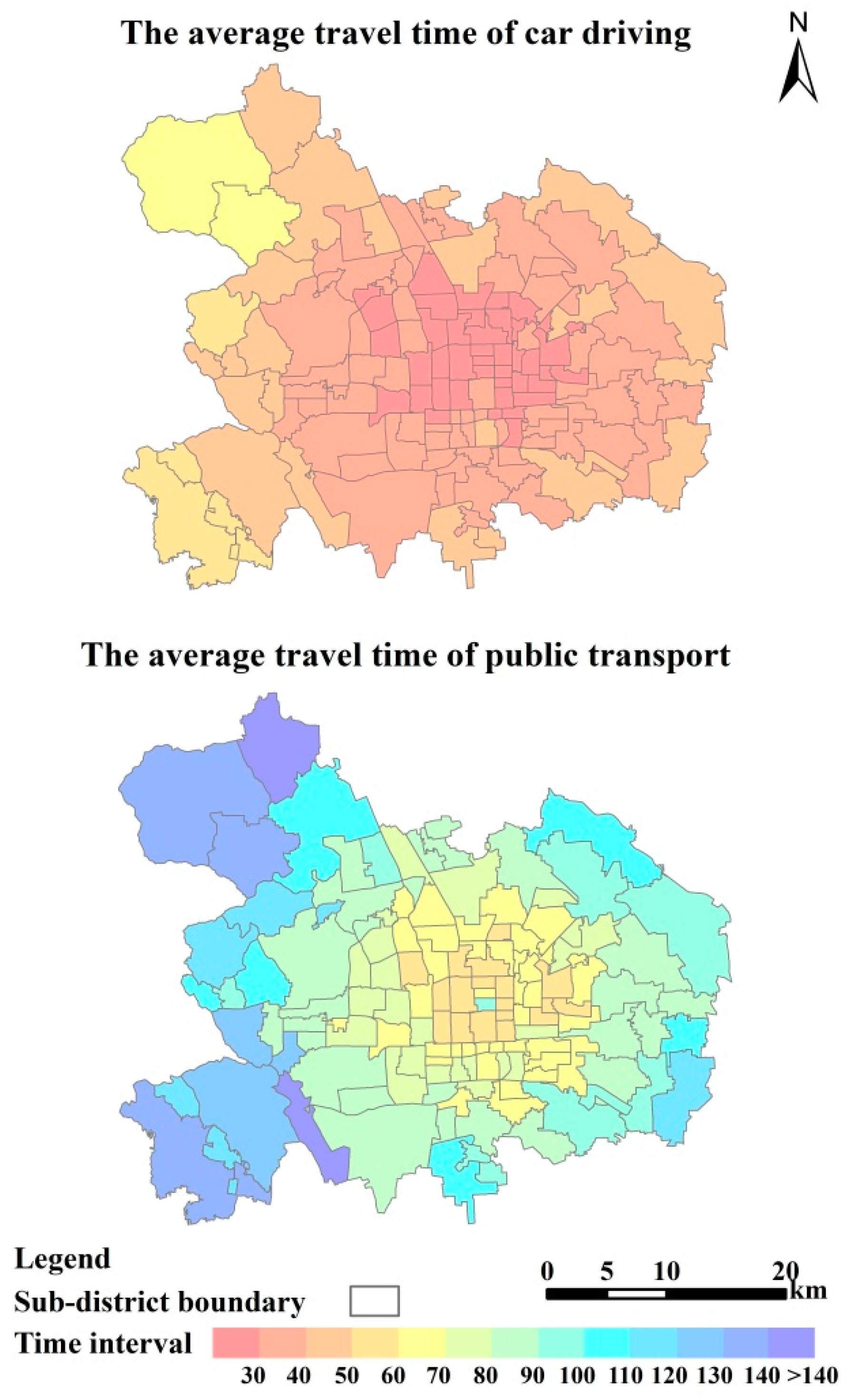
3.1. The Average Travel Time of Sub District

Baidu map is a platform for users to provide travel-related services. It can also provide users with travel planning and time-consuming requirements according to real-time road conditions. Therefore, the travel time via car and public transport is collected from Baidu map API under the support of a digital map and dynamic road conditions. This travel time will give an objective value considering the road congestion and traffic flow, so as to avoid a lot of road network processing work, and the results will more reliable.
The travel time of residents is collected with taking the sub-district as the original point (O) and entrances of parks as the destination (D). Thus, we get the travel time of the sub district-park pairs. In detail, we get the travel time of car driving and public transportation (which includes underground transportation and ground transportation) of these OD pairs, respectively.
The average travel time of a sub-district represents the average time from each sub-district to all of its accessed parks. This value can explain the cost consumption of the sub-district’s access to the urban park. This is calculated for car driving and for public transport, respectively. The formulas are as follows.
  A T i c =     1 n j n T i , j c
A T i p = 1 n j n T i , j p
where A T i c and A T i p denote the average travel time of sub-district i under the mode of private car and public transportation, respectively. T i , j c and T i , j p are the travel time of private car and public transport from sub-district i to park j , respectively, and n is the number of parks that sub-district i can access.

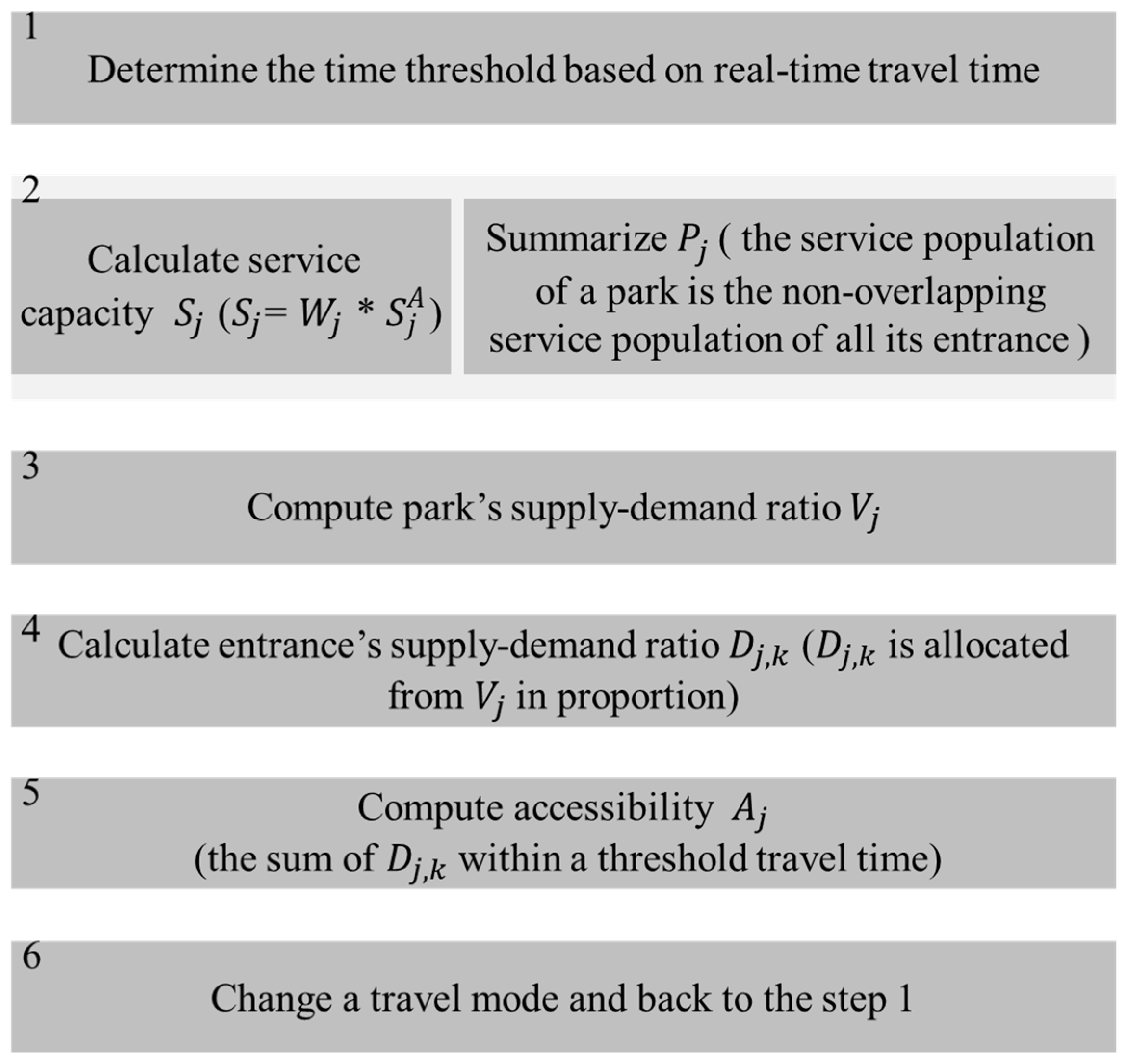
3.2. The Model for Measuring Spatial Accessibility

3.2.1. The Traditional 2SFCA Method

The two-step floating catchment area (2SFCA) method is performed in this article to measure the accessibility value. The core idea of the 2SFCA method is to search the floating catchment area (FCA) twice, once at the supply point and once at the demand point, so this method includes the following two steps [30,31].
In the first step, supply point j is taken as the center and search all demand points i within j ’s search domain, then we can calculate the supply-demand ratio   V j .
V j = S j d j , i < d 0 P i
In this expression, V j represents the supply-demand ratio of park j , S j is the service capacity of supply j , and   d j , i is the travel cost between supply point j and demand point i . d 0 represents the threshold for the range of supply point services, which usually expressed in time or distance. P i is the requirement of unit i which falls within the scope of the search domain of the supply point j .
In the second step, for each demand point i , we search all the supply points in the search domain, and the supply–demand ratio V j of these supply points is added to obtain the accessibility of demand point i .
A i = d i , j < d 0 V j = d i , j < d 0 S j d j , i < d 0 P i
A i is the accessibility of demand unit i . A high A i value indicates that the demand unit has high accessibility.
In the accessibility measurement of urban park space, we used geometric centroids or centers to replace the park itself as the demand point may produce bias. A brief reason is given in introduction and here we will explain this in further detail. Many parks in reality have gates and only allow people to enter from the entrance. Figure 3 is a conceptual map demonstrating this. We generally think that to reach the entrance is to reach that facility. Therefore, the distance from the entrance to the center needs to be excluded in the experiment. In addition, when searching the FCA, if some areas of the park are within the catchment area but do not reach the center (such as J1, J3 in Figure 4), they will not be included in the catchment area. Meanwhile, when the center of the park is within the scope of the catchment area and the whole park is not fully included in the search domain (such as J2 in Figure 4), the whole park will still be included in the calculation.

3.2.2. The Modified 2SFCA Method

According to the above, for this article, we took the entrances of the park as the destination. So, in the first step of 2SFCA, the searching process was implemented from each entrance and the overall supply–demand ratio of a park was proportionally distributed to each entrance. In the second step, the target of the searching process was the entrances of the park instead of centroids and the supply–demand ratio of entrances was used to calculate accessibility. In this article, we introduced park grade and suggested that service capacity S j is a function of size and grade, which is similar to the literature of Xing et al., who used park size and function to represent service capacity [44]. It is worth mentioning that park function and park grade are a similar evaluation of the overall service capacity of a park, and park grade is converted to corresponding numbers, for example, 5A grade is converted as 5. According to the obtained travel data and the existing papers [46,47], we defined three travel modes when studying the spatial accessibility: car driving, public transport and car-public transport mixed travel mode (the mixed mode for short). It should be mentioned that the mixed mode was proposed to divide the population into residents choosing car to travel or not. The proportion was provided from the Beijing Transportation Research Center (2017) [48], which indicated that 32.3% residents prefer car to travel in the travel structure. For residents using car to travel, the searching threshold was similar to car driving mode and the demand-population was residents who prefer car. As for the other residents, the searching threshold was the same as public transport mode.
The improved model is as follows and the framework is shown in Figure 5.
Step one is to calculate the supply-demand ratio:
V j = S j P j = W j S j A P j
In this formula, V j is the supply-demand ratio of park j . S j A is the area of park j , units in km 2 , and W j is the grade of park j . P j represents the total demand population falling within the scope of search domain of all entrances of park j . The formulas for each mode are as follows.
P j c = i k { i | d k , i < d 0 c } P i
P j p = i k { i | d k , i < d 0 p } P i
P j m = i k { i | d k , i < d 0 c } P i C + i k { i | d k , i < d 0 p } P i N C
where P j c ,   P j p , P j m represent the total demand population park j under car driving, public transport and car-public transport mixed mode, respectively.   d k , i indicates the travel cost between park j ’ entrance k and sub-district i , and d 0 c , d 0 p are the searching threshold of car driving and public transport. P i represents the total population of demand i . Similarly,   P i C ,   P i N C respectively represent the population prefer using car to travel and not.
In order to proportionally allocate the calculated supply–demand ratio of park j to each of its entrances, the following formula is required. By this formula, V j can be proportionally allocated to each entrance and it can ensure that the sum of the supply–demand ratio of each entrance can equal the value of the supply–demand ratio of park j ( V j ). The formula implements the assignment from the whole to the individual.
D j , k = V j P j , k k = 1 n P j , k
where D j , k is the supply-demand ratio of the entrance k in park j , which will be used to calculate the accessibility in the next step. It is weighted from V j and this weight is obtained by the ratio of the population of park j ’s entrance k to the total population of all entrances of park j .
Step two is to calculate the accessibility value.
A j = d < d 0 D j , k
where A j indicates accessibility in mode , and d 0 indicates the search threshold in the mode . Note that in the mixed mode, the searching range is the union of car driving and public transport mode.

3.3. Spatial Autocorrelation Analysis of Accessibility

The spatial analysis method, like Getis-Ord Gi * [49] and spatial autocorrelation analyses [50], can be utilized to describe the spatial distribution regularities of objects and there are studies in which spatial autocorrelation analyses were used for the accessibility scores [47,51]. Spatial autocorrelation refers to the statistical correlation between certain attribute values of geographical things that are distributed in different spatial locations, which is usually represented by global spatial autocorrelation and local spatial autocorrelation [52,53].
Global spatial autocorrelation analysis measures the relationship between attribute values of adjacent spatial distribution objects, which is represented by Moran’ I [54].
I = n i = 1 n j = 1 n w i j ( y i y ¯ ) ( y j y ¯ ) ( i = 1 n j = 1 n w i j ) i = 1 n ( y i y ¯ ) 2
The Z-score is used to test the significance of Moran’ I. When | Z | > 1.96, it means they have spatial autocorrelation.
Global spatial autocorrelation analysis is used to test the global correlation under only one trend. However, due to the spatial heterogeneity of control objects [53], local spatial autocorrelation analysis is used to find out whether there is spatial autocorrelation in a local space. For each distribution object in the space, the formula is as follows [54],
I i = y i y ¯ S 2 j n w i j ( y j y ¯ )
The Z value is also used to test the significance of local spatial autocorrelation. In Formulas (11) and (12), n is the number of space units,   y i and y j are the attribute values of space objects at points i and j , respectively. y ¯ is the average value. The spatial weight matrix element w i j is the connection between i and j points of the spatial object.

4. Results

4.1. Travel Time

Travel time is an important factor affecting accessibility. The sub-district is regarded as the original point (O), and entrances of parks are regarded as a destination (D). We get the travel time of each sub district-park (OD) pair, and then conduct a multi-perspective analysis of travel time. According to the statistics, the mean travel time between OD pairs for car travel is 35 min, with a minimum value of 1 min and a maximum value of 91 min. In contrast, the mean travel time of OD pairs for public transport is 80 min, with a minimum value of 14 min, and the maximum value is 316 min. It should be noted that OD pairs without public transport travel route is excluded. We can find that the mean time of public transport is about 2.29 times that of car driving.
Then, we calculate the travel situation from the sub-district perspective by using the average travel time of sub district, which represents the average time from each sub-district to all of its accessed parks. Figure 6 is a histogram and cumulative probability picture. The X-axis is travel time and the Y-axis is the number of sub-districts. We can find that for car travel, the calculated average travel time of sub-districts is within 70 min, of which 30–40 min is the most common, accounting for 47.37% of the total number of sub-districts. The second most common is the 20–30 min period, accounting for 30.83% of the total number of sub-districts, while the 40–50, 50–60, and 60–70 periods are relatively less common, comprising 17.29%, 3.01%, 1.50% of the sub-districts, respectively. Meanwhile, the calculated travel time for public transport is between 60 and 180 min, mainly within 60–90 min. The time period with the largest proportion is 70–80 min, accounting for 28.57% of the total number of sub-districts. The number of sub-districts in the other periods of time is relatively scattered. Figure 6 also shows that 95% of the sub-districts hold an average travel time within 50 min with car driving, while the minimum average travel time of public transport is 53 min, and 93.23% of the sub-districts can be reached by public transport within 120 min. Figure 7 is the spatial distribution of the average travel time under different travel methods. This clearly shows that the time increases from the center to the periphery. The picture above in Figure 7 shows the average car driving time of the sub-district and the picture below shows the calculated travel time in public transport. This chart is divided into 13 bands, with an interval of 10 min starting from 30 min. The color from red to blue-purple indicates that the average travel time of the sub-district increases gradually. We can find some spatial disparity information from it. Sub-districts in the top picture are almost filled with red and orange color, which demonstrates the short average travel time and in the bottom picture, sub districts are mainly filled with the long average travel time color, such as cyan and blue-purple.

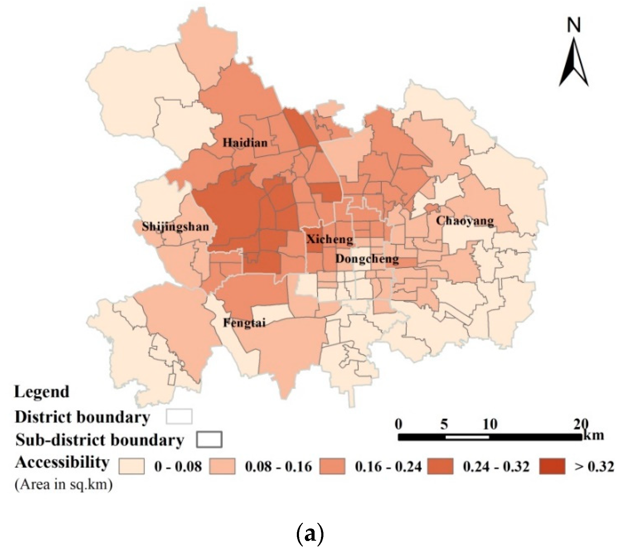
4.2. Accessibility of Different Transport Mode

According to the obtained travel time between OD pairs, the improved 2SFCA method is used to calculate the accessibility value between the sub-district and parks. Based on the statistics of travel time between OD pairs and the reference of existing papers [47], we choose the mean time as the travel threshold, as it represents the average travel situation of the research object. We set out three travel modes for research in Section 3.2, so we get the accessibility of car driving (Figure 8a), public transport (Figure 8b), and the mixed mode (Figure 8c), respectively. We divide the accessibility results value into five levels, namely the highest level (>0.32), the high level (0.24–0.32), the medium level (0.16–0.24), the low level (0.08–0.16) and the lowest level (0–0.08). In Figure 8, dark color indicates high accessibility while light color indicates low accessibility. The value represents the area of park per ten thousand people.
In the distribution figure of the car driving mode (Figure 8a), we can see that it contains four levels of accessibility, and the highest level is excluded. The reason for this is that the car driving mode can get a wide scope in a mean-time threshold, which means there will be more residents to become the service objects, thus the supply-demand ratio is decreased, finally leading to a low accessibility result. The accessibility spatial distribution takes the south of Haidian District as the center and spreads around in a circle structure. Within the defined threshold, the accessibility of car driving is high in the central to northwestern area of the study area, while in the peripheral sub-districts with a sparse road network, the accessibility of the park is relatively low. There are thirteen sub-districts with a high accessibility level (0.24–0.32) in the south of Haidian District. The sub-districts with the lowest accessibility level (0–0.08) have an incompact distribution, and are mainly distributed in the east and south of Chaoyang District, and the east of Fengtai District. There are also a few in the northwest of Haidian District, the southwest of Fengtai District, the south of Dongcheng and Xicheng District.
Figure 8b shows the spatial distribution of public transport modes. It is worth noting that in this figure, the accessibility values of Wenquan Town Sub-district, Shangzhuang Town Sub-district and Sujiatuo Town sub-district in the northwest of Haidian District, Changxindian sub-district and Wanpingcheng sub-district in Fengtai District are 0 (which have been emphasized with yellow boundary line in Figure 8b). The reason is that these sub-districts have no traffic plan under the average travel time of 80 min of public transportation—that is to say, it is impossible to reach any research park from these sub-districts within 80 min or that there is no public transport route between these sub-districts and parks. There is one sub-district with the highest level in Haidian District and seventeen sub-districts with a high accessibility level, which is four more than car driving mode but the distribution is more disperse than that. High accessibility sub-districts are mainly distributed in the centre to the north of the study area, such as the north of Dongcheng District and Xicheng District, the southeast of Haidian District and the west of Chaoyang District, which are old urban areas in Beijing. The distribution area of low accessibility is similar to that of the car driving mode.
Figure 8c shows the spatial difference in accessibility under the mixed travel model. The number of sub-districts with the highest accessibility level is ten. This number is much larger than that in the car driving and public transport mode. These sub-districts are mainly concentrated in the south of Haidian District. Obviously, the accessibility of the park in three modes has spatial heterogeneity. We can see that compared with the first two modes, the mixed mode has more obvious accessibility advantages. It is clear that the range of the highest and high accessibility level sub-districts under the mixed mode is more widely distributed. In addition, the mixed mode has less of the lowest accessibility level sub-districts, with 16 in the mixed mode, 35 in the public transport mode and 38 in the car driving mode, though these sub-districts are mostly distributed in the peripheral area.
From the macro level, the three travel modes all reflect the same rule. That is, the regions with high accessibility are distributed from the south of Haidian District to Xicheng District and Dongcheng District. With the range moving to the peripheral area, the accessibility level also decreases. Combined with the sub-district average travel time distribution, we can find that this is closely related to the increase in travel time. This also proves that travel time is a significant factor affecting accessibility.

4.3. The Spatial Autocorrelation Results of Different Transport Modes in Accessibility

Based on the above results, the spatial autocorrelation analysis of accessibility is applied. We use the queen consistency weight method to calculate the global spatial autocorrelation index Moran’ I, and generate the local autocorrelation clustering graph. These steps are carried out in GeoDA, which is a geography software developed by Dr. Luc Anselin and his team. Table 1 shows the results of global spatial autocorrelation analysis in three modes. Figure 9 shows the corresponding global spatial autocorrelation scatter in different modes. It can be seen from Table 1 that in each mode, Moran’ I index is greater than 0, the Z-value is greater than 1.96, and the calculation results pass the Z-value test (p-value is 0.01 < 0.05). This shows that, in the central area in Beijing, the accessibility of the sub-districts to the 3A level and above parks has a positive spatial correlation. This means that the high accessibility is adjacent to the high accessibility sub-districts, and the low accessibility is adjacent to the low accessibility sub-districts. Local autocorrelation analysis is used to identify high and low level spatial clustering of park accessibility as well as spatial outlying sub-districts in the study area, and the Local Indication of Spatial Association (LISA) cluster map is generated, as shown in Figure 10. Red is High-High value clustering (H-H), blue is Low-Low value clustering (L-L), purple and pink are outliers (L-H, H-L). Although in the three modes, the spatial distribution of H-H value clustering and L-L value clustering is slightly different, the overall distribution is consistent. As shown in Figure 10, H-H values are mainly distributed in the southeast of Haidian District, Dongcheng District and Xicheng District, while L-L values are mainly distributed in the peripheral sub-districts. The rest of study area is distributed with outliers and no significant sub-districts.

5. Discussion

In this paper, with the support of real-time travel data, we first calculated the average travel time of the sub-district park pairs. The average travel time from the sub-district to parks implies a spatial pattern that the travel time increases from the center of the study area to the peripheral area. The results show that sub-districts’ average travel times in the car driving mode are mostly concentrated in the 30–40 min period, while in public transport mode, the times are most concentrate in 60–90 min period. Through the histogram of Figure 6 and the spatial distribution of Figure 7, it can be seen that the car driving mode has a more obvious time–space compression effect than the public transportation mode. This finding is similar to the results of Wang et al.’s analysis on the travel time of scenic spots [51].
In terms of accessibility results based on the modified 2SFCA method, we can find that the sub-districts with high accessibility level in car driving mode are mostly distributed in the south of Haidian District. These sub-districts are located near the third and fourth ring roads in Beijing, so the traffic there is convenient. This is one of the reasons for the highest accessibility. What is more, the Summer Palace (5A grade park) and Yuyuantan Park (4A grade park) are around them, so the proximity to the demand point is also a reason. Meanwhile, the results show that within the third ring road, the accessibility value remains relatively low, in spite of dense parks. Through the analysis of travel time and formula, we found that within the search threshold range, parks here can serve a large range of demanders, but the service capacity of the park is relatively low, which results in a lower supply–demand ratio and furthermore a lower accessibility result. The sub-districts with the lowest accessibility level are mostly distributed in the eastern peripheral area, as they are far away from the Beijing ring road and require a long travel time. In addition, these places are densely populated but sparsely distributed with parks.
In the public transport mode, the dense distribution of public transport routes corresponds to greater accessibility, and vice versa. High accessibility sub-districts are mainly distributed in the central to the north of the study area, because these areas are old urban areas, with the most complete public transport facilities and the densest metro and public transport lines. Compared with these areas, the south of the study area has relatively low accessibility. This demonstrates that the development of the northern part of Beijing’s central urban area is better than that of the southern part, which further forms a more complete transportation infrastructure.
The mixed mode has the highest number of the highest accessibility level sub-districts. This is because in the mixed mode, it not only takes advantage of the high speed of the third ring road and the fourth ring road, but also enjoys the advantages of perfect public transport infrastructure. In this mode, residents can access more parks, so the accessibility is higher. Obviously, the accessibility is higher in the west of the study area than in the east, even though the economic development of the east is better than that of the west. This is because the eastern part is mainly distributed with large business districts. The parks located there are small and the population is dense. Meanwhile, the western part has more large parks. Comprehensively analyzing this, the sub-districts with lowest accessibility are distributed in the peripheral area, which is closely related to the limited road network and public transport and to the sparse distribution of parks. Therefore, accessibility can be improved by increasing the traffic capacity of this part of the area. The findings of this study on the spatial disparity in the accessibility of parks are similar to Zhang et al. on the spatial disparity in the accessibility of churches [55]. In addition, we further found that higher accessibility can be obtained in the mixed mode of travel. Therefore, managers can improve the accessibility of residents by encouraging them to travel by different means of transportation.
The spatial autocorrelation analysis shows that the accessibility of the park has a positive globe spatial correlation. The LISA cluster maps of the three modes show that the H-H value clustering area and the L-L value clustering area are respectively distributed in some inner city and marginal areas. This indicates a significant imbalance in access to the resources. This is closely related to the spatial distribution of park resources as depicted in Figure 1. Thus, it can provide information for planners in their future designs in marginal areas.

6. Conclusions

Many accessibility measuring methods are utilized for better understanding the satisfaction of residents’ demand about parks. However, the representation of entrances of large or medium-sized parks has been ignored in the literature for a long time. In this study, we took the entrances of parks as the destination for analyzing the accessibility of parks. Taking the central area of Beijing as the study area, the 2SFCA method was modified according to the characteristic of large or medium-sized parks with entrances. As the travel time is an important element for evaluating accessibility, real-time travel time from Baidu maps was utilized. We first got the travel time between sub-district (O) and the entrance of parks (D) and in order to reveal the travel ability of sub-district to all accessed parks, the average travel time was calculated. Then, the mean time of OD pairs was utilized to measure the accessibility to parks under three defined modes with the modified 2SFCA method. The research shows that there was better accessibility satiation under the mixed mode, which provides information and support for advocating that residents have different means of transportation, such as public transport. Finally, Moran’ I index and LISA cluster map are used to detect global spatial autocorrelation and local spatial autocorrelation respectively.
The results of this study can provide information for future urban planning. In addition, the research method of this paper can also be considered in other facilities with similar characteristics. However, there are some limitations in our work. The first limitation is that the population in this paper is census data, which is mainly aimed at the permanent residents of the region, without considering the situation of tourists. In future research, we can add the big data based on location-based services, such as microblogs, to combine the permanent population with domestic and foreign tourists for further in-depth research. Second, the edge effect is not considered in this study. Thus, the accessibility might be underestimated when residents access parks which are just outside of the study area but can serve the study area under the time threshold. Third, this article considers car driving and public transport as the travel tool, and the mixed mode also assumes that residents, excluding those who prefer car driving, all use public transport to travel. Other modes such as walking and cycling can be analyzed as separate modes and added into the mixed mode in follow-up studies. Fourth, in this paper, geographical centroids are used in sub-districts as demand points. Although this is widely used, it may still cause errors if the sub-districts are large or the population distribution is very uneven. Therefore, we will consider this aspect in future work, such as using a more appropriate unit for the further experiment.

Author Contributions

Conceptualization, J.Q. and S.S.; methodology, J.Q. and D.Y.; validation, Y.L., J.Z.; investigation, S.S.; writing—original draft preparation, J.Q.; writing—review and editing, J.Q., D.Y. and Y.L.; Supervision, J.Z. All authors have read and agreed to the published version of the manuscript.

Funding

This research was funded by The Open Project Program of the State Key Laboratory of Virtual Reality Technology and Systems, Beihang University (Grant No.01119220010011).

Acknowledgments

We are grateful for the valuable comments of Yong Gao and the anonymous reviewers.

Conflicts of Interest

The authors declare no conflict of interest.

References

  1. Shin, D.; Lee, K. Use of remote sensing and geographical information systems to estimate green space surface-temperature change as a result of urban expansion. Landsc. Ecol. Eng. 2005, 1, 169–176. [Google Scholar] [CrossRef]
  2. Sun, F.; Xiang, J.; Tao, Y.; Tong, C.; Che, Y. Mapping the social values for ecosystem services in urban green spaces: Integrating a visitor-employed photography method into SolVES. Urban For. Urban Green. 2019, 38, 105–113. [Google Scholar] [CrossRef]
  3. Hand, K.; Freeman, C.; Seddon, P.; Recio, M.; Stein, A.; Van Heezik, Y. The importance of urban gardens in supporting children’s biophilia. Proc. Natl. Acad. Sci. USA 2017, 114, 274–279. [Google Scholar] [CrossRef] [PubMed] [Green Version]
  4. Wu, C.; Ye, X.; Du, Q.; Luo, P. Spatial effects of accessibility to parks on housing prices in Shenzhen, China. Habitat Int. 2017, 63, 45–54. [Google Scholar] [CrossRef]
  5. Qiu, G.Y.; Zou, Z.; Li, X.; Li, H.; Guo, Q.; Yan, C.; Tan, S. Experimental studies on the effects of green space and evapotranspiration on urban heat island in a subtropical megacity in China. Habitat Int. 2017, 68, 30–42. [Google Scholar] [CrossRef]
  6. Kroeger, T.; Escobedo, F.J.; Hernandez, J.L.; Varela, S.; Delphin, S.; Fisher, J.R.; Waldron, J. Reforestation as a novel abatement and compliance measure for ground-level ozone. Proc. Natl. Acad. Sci. USA 2014, 111, E4204–E4213. [Google Scholar] [CrossRef] [PubMed] [Green Version]
  7. Bowler, D.E.; Buyungali, L.M.; Knight, T.M.; Pullin, A.S. Urban greening to cool towns and cities: A systematic review of the empirical evidence. Landsc. Urban Plan. 2010, 97, 147–155. [Google Scholar] [CrossRef]
  8. Maimaitiyiming, M.; Ghulam, A.; Tiyip, T.; Pla, F.; Latorre-Carmona, P.; Halik, Ü.; Sawut, M.; Caetano, M. Effects of green space spatial pattern on land surface temperature: Implications for sustainable urban planning and climate change adaptation. ISPRS J. Photogramm. Remote Sens. 2014, 89, 59–66. [Google Scholar] [CrossRef] [Green Version]
  9. Silveira, I.H.D.; Junger, W.L. Green spaces and mortality due to cardiovascular diseases in the city of Rio de Janeiro. Rev. Saude Publica 2018, 52. [Google Scholar] [CrossRef] [Green Version]
  10. Picavet, H.S.J.; Milder, I.; Kruize, H.; de Vries, S.; Hermans, T.; Wendel-Vos, W. Greener living environment healthier people? Exploring green space, physical activity and health in the Doetinchem Cohort Study. Prev. Med. 2016, 89, 7–14. [Google Scholar] [CrossRef]
  11. Ward Thompson, C.; Roe, J.; Aspinall, P.; Mitchell, R.; Clow, A.; Miller, D. More green space is linked to less stress in deprived communities: Evidence from salivary cortisol patterns. Landsc. Urban Plan. 2012, 105, 221–229. [Google Scholar] [CrossRef] [Green Version]
  12. Krellenberg, K.; Welz, J.; Reyes-Päcke, S. Urban green areas and their potential for social interaction–A case study of a socio-economically mixed neighbourhood in Santiago de Chile. Habitat Int. 2014, 44, 11–21. [Google Scholar] [CrossRef]
  13. Harnik, P.; Welle, B.J. Measuring the Economic Value of a City Park System; Trust for Public Land: Washington, DC, USA, 2009. [Google Scholar]
  14. Kong, F.; Nakagoshi, N. Spatial-temporal gradient analysis of urban green spaces in Jinan, China. Landsc. Urban Plan. 2006, 78, 147–164. [Google Scholar] [CrossRef]
  15. Chen, M.; Li, T. Study on development strategy for country parks in Shanghai. Chin. Landsc. Arch. 2009, 25, 10–13. (In Chinese) [Google Scholar]
  16. Hong, W.; Yang, C.; Chen, L.; Zhang, F.; Shen, S.; Guo, R. Ecological control line: A decade of exploration and an innovative path of ecological land management for megacities in China. J. Environ. Manag. 2017, 191, 116–125. [Google Scholar] [CrossRef]
  17. Boone, C.G.; Buckley, G.L.; Grove, J.M.; Sister, C. Parks and people: An environmental justice inquiry in Baltimore, Maryland. Ann. Assoc. Am. Geogr. 2009, 99, 767–787. [Google Scholar] [CrossRef]
  18. Xiao, Y.; Wang, Z.; Li, Z.; Tang, Z. An assessment of urban park access in Shanghai—Implications for the social equity in urban China. Landsc. Urban Plan. 2017, 157, 383–393. [Google Scholar] [CrossRef]
  19. Rigolon, A. A complex landscape of inequity in access to urban parks: A literature review. Landsc. Urban Plan. 2016, 153, 160–169. [Google Scholar] [CrossRef]
  20. Song, Z.; Chen, W.; Zhang, G.; Zhang, L. Spatial accessibility to public service facilities and its measurement approaches. Progr. Geogr. 2010, 29, 1217–1224. (In Chinese) [Google Scholar]
  21. Lee, G.; Hong, I. Measuring spatial accessibility in the context of spatial disparity between demand and supply of urban park service. Landsc. Urban Plan. 2013, 119, 85–90. [Google Scholar] [CrossRef]
  22. Hansen, W.G. How accessibility shapes land use. J. Am. Plan. Assoc. 1959, 25, 73–76. [Google Scholar] [CrossRef]
  23. Morris, J.M.; Dumble, P.L.; Wigan, M.R. Accessibility indicators for transport planning. Transp. Res. Part A Gen. 1979, 13, 91–109. [Google Scholar] [CrossRef]
  24. Batty, M. Urban Modelling: Algorithms, Calibrations, Predictions; Cambridge University Press: Cambridge, UK, 1976. [Google Scholar]
  25. Deboosere, R.; El-Geneidy, A. Evaluating equity and accessibility to jobs by public transport across Canada. J. Transp. Geogr. 2018, 73, 54–63. [Google Scholar] [CrossRef]
  26. Kong, X.; Liu, Y.; Wang, Y.; Tong, D.; Zhang, J. Investigating public facility characteristics from a spatial interaction perspective: A case study of Beijing hospitals using taxi data. ISPRS Int. Geo-Inf. 2017, 6, 38. [Google Scholar] [CrossRef]
  27. Cheng, L.; Caset, F.; De Vos, J.; Derudder, B.; Witlox, F. Investigating walking accessibility to recreational amenities for elderly people in Nanjing, China. Transp. Res. Part D-Transp. Environ. 2019, 76, 85–99. [Google Scholar] [CrossRef]
  28. Johnston, R.J. The Dictionary of Human Geography; Basil Blackwell: Oxford, UK, 1981. [Google Scholar]
  29. Ingram, D.R. The concept of accessibility: A search for an operational form. Reg. Stud. 1971, 5, 101–107. [Google Scholar] [CrossRef]
  30. Radke, J.; Mu, L. Spatial decompositions, modeling and mapping service regions to predict access to social programs. Ann. GIS 2000, 6, 105–112. [Google Scholar] [CrossRef]
  31. Luo, W.; Wang, F. Measures of spatial accessibility to health care in a GIS environment: Synthesis and a case study in the Chicago Region. Environ. Plan. B Plan. Des. 2003, 30, 865–884. [Google Scholar] [CrossRef] [Green Version]
  32. Luo, W.; Qi, Y. An enhanced two-step floating catchment area (E2SFCA) method for measuring spatial accessibility to primary care physicians. Health Place 2009, 15, 1100–1107. [Google Scholar] [CrossRef]
  33. Kanuganti, S.; Sarkar, A.K.; Singh, A.P. Evaluation of access to health care in rural areas using enhanced two-step floating catchment area (E2SFCA) method. J. Transp. Geogr. 2016, 56, 45–52. [Google Scholar] [CrossRef]
  34. Dai, D. Black residential segregation, disparities in spatial access to health care facilities, and late-stage breast cancer diagnosis in metropolitan Detroit. Health Place 2010, 16, 1038–1052. [Google Scholar] [CrossRef] [PubMed]
  35. Dai, D.; Wang, F. Geographic disparities in accessibility to food stores in southwest Mississippi. Landsc. Urban Plan B. 2011, 38, 659–677. [Google Scholar] [CrossRef]
  36. Li, L.; Du, Q.; Ren, F.; Ma, X. Assessing spatial accessibility to hierarchical urban parks by multi-types of travel distance in Shenzhen, China. Int. J. Environ. Res. Public Health 2019, 16, 1038. [Google Scholar] [CrossRef] [PubMed] [Green Version]
  37. Gu, X.; Tao, S.; Dai, B. Spatial accessibility of country parks in Shanghai, China. Urban For. Urban Green. 2017, 27, 373–382. [Google Scholar] [CrossRef]
  38. Li, Z.; Wei, H.; Wu, Y.; Su, S.; Wang, W.; Qu, C. Impact of community deprivation on urban park access over time: Understanding the relative role of contributors for urban planning. Habitat Int. 2019, 92, 102031. [Google Scholar] [CrossRef]
  39. Wei, F. Greener urbanization? Changing accessibility to parks in China. Landsc. Urban Plan. 2017, 157, 542–552. [Google Scholar] [CrossRef]
  40. Guo, S.; Song, C.; Pei, T.; Liu, Y.; Ma, T.; Du, Y.; Chen, J.; Fan, Z.; Tang, X.; Peng, Y.; et al. Accessibility to urban parks for elderly residents: Perspectives from mobile phone data. Landsc. Urban Plan. 2019, 19, 103642. [Google Scholar] [CrossRef]
  41. Xing, L.; Liu, Y.; Wang, B.; Wang, Y.; Liu, H. An environmental justice study on spatial access to parks for youth by using an improved 2SFCA method in Wuhan, China. Cities 2020, 96, 102405. [Google Scholar] [CrossRef]
  42. Bryant, J., Jr.; Delamater, P.L. Examination of spatial accessibility at micro-and macro-levels using the enhanced two-step floating catchment area (E2SFCA) method. Ann. GIS 2019, 25, 219–229. [Google Scholar] [CrossRef] [Green Version]
  43. Xing, L.; Liu, Y.; Liu, X.; Wei, X.; Mao, Y. Spatio-temporal disparity between demand and supply of park green space service in urban area of Wuhan from 2000 to 2014. Habitat Int. 2018, 71, 49–59. [Google Scholar] [CrossRef]
  44. Xing, L.; Liu, Y.; Liu, X. Measuring spatial disparity in accessibility with a multi-mode method based on park green spaces classification in Wuhan, China. Appl. Geogr. 2018, 94, 251–261. [Google Scholar] [CrossRef]
  45. Dony, C.C.; Delmelle, E.M.; Delmelle, E.C. Re-conceptualizing accessibility to parks in multi-modal cities: A variable-width Floating Catchment Area (VFCA) method. Landsc. Urban Plan. 2015, 143, 90–99. [Google Scholar] [CrossRef]
  46. Mao, L.; Nekorchuk, D. Measuring spatial accessibility to healthcare for populations with multiple transportation modes. Health Place 2013, 24, 115–122. [Google Scholar] [CrossRef] [PubMed]
  47. Cheng, G.; Zeng, X.; Duan, L.; Lu, X.; Sun, H.; Jiang, T.; Li, Y. Spatial difference analysis for accessibility to high level hospitals based on travel time in Shenzhen, China. Habitat Int. 2016, 53, 485–494. [Google Scholar] [CrossRef] [Green Version]
  48. Beijing Transportation Research Center. 2017 Beijing Transport Annual Report; Beijing Transportation Research Center: Beijing, China, 2017. (In Chinese) [Google Scholar]
  49. Wen, C.; Albert, C.; Von Haaren, C. Equality in access to urban green spaces: A case study in Hannover, Germany, with a focus on the elderly population. Urban For. Urban Green. 2020, 55, 126820. [Google Scholar] [CrossRef]
  50. Lv, T.; Cao, Y. Construction of spatial autocorrelation method of spatial-temporal proximity and its application: Taking regional economic disparity in the Yangtze River Delta as a case study. Geogr. Res. 2010, 29, 351–360. (In Chinese) [Google Scholar]
  51. Wang, L.; Cao, X.; Li, T.; Gao, X. Accessibility comparison and spatial differentiation of Xi’an scenic spots with different modes based on baidu real-time travel. Chin. Geogr. Sci. 2019, 29, 848–860. [Google Scholar] [CrossRef] [Green Version]
  52. Moran, P.A. The interpretation of statistical maps. J. R. Stat. Soc. Ser. B Stat. Methodol. 1948, 10, 243–251. [Google Scholar] [CrossRef]
  53. Anselin, L. Local indicators of spatial association—LISA. Geogr. Anal. 1995, 27, 93–115. [Google Scholar] [CrossRef]
  54. Wang, F. Quantitative Methods and Application in GIS; CRC Press: Boca Raton, FL, USA, 2006. [Google Scholar]
  55. Zhang, K.; Zhang, S. Accessibility analysis of protestant churches in Shanghai, China. GeoJournal 2019, 1–10. Available online: https://link.springer.com/article/10.1007/s10708-019-10089-z (accessed on 15 September 2020). [CrossRef]
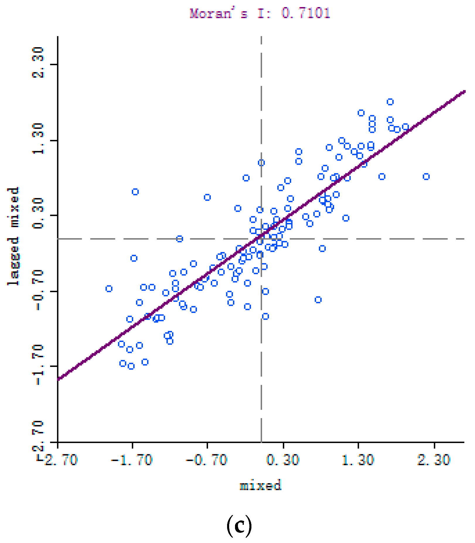
Figure 1. Study area and the location of parks.
Sustainability 12 07618 g001
Figure 2. Spatial distribution of public transport stops.
Sustainability 12 07618 g002
Figure 3. A conceptual map of the route between demand point (sub-district) and supply point (park), where “ e ” represent “ entrance ” and (a), (b), (c), (d) are the available routes between sub-district and park in theoretical.
Sustainability 12 07618 g003
Figure 4. The searching scope when treated geometric centroids as destination. (J1, J2, J3 represent demand points, red points are the entrances while the yellow point is the geometric centroid.).
Sustainability 12 07618 g004
Figure 5. The framework of the modified 2SFCA method based on real-time travel time data and multi-entrances.
Sustainability 12 07618 g005
Figure 6. The histogram and cumulative probability picture of the average travel time of sub-districts.
Sustainability 12 07618 g006
Figure 7. A visual map of the average travel time of sub-districts in car driving and public transport way, respectively.
Sustainability 12 07618 g007
Figure 8. The spatial pattern of accessibility via different travel modes in urban area of Beijing, China. (a) The accessibility of car driving mode; (b) the accessibility of public transport mode; (c) the accessibility of the mixed mode.
Sustainability 12 07618 g008aSustainability 12 07618 g008b
Figure 9. The Moran scatter diagrams of accessibility index in different modes in urban area of Beijing, China. (a) Car driving mode; (b) public transport mode; (c) the mixed mode.
Sustainability 12 07618 g009aSustainability 12 07618 g009b
Figure 10. Local Indication of Spatial Association (LISA) cluster map of accessibility index in urban area of Beijing, China. (a) Car driving mode; (b) public transport mode; (c) the mixed mode.
Sustainability 12 07618 g010aSustainability 12 07618 g010b
Table 1. The results of global spatial autocorrelation analysis.
Travel ModeMoran’ IZ-Valuep-Value
Car driving0.744313.61850.01
Public transport0.599110.16470.01
Mixed0.710112.18870.01

