1. Introduction
According to the United Nations [
1], the proportion of the world population living in cities is expected to increase from 55% in 2018 to 68% by 2050. As the city becomes more densely populated, sustainable development is more indispensable than ever, in order to tackle problems such as mitigation of climate change and enhancement of the quality of life of citizens in the city.
Amid these challenges, urban green space is expected to provide positive effects on different aspects in the city, such as reduction of air and water pollution [
2,
3,
4], mitigation of urban heat effect [
5,
6], and various aspects of public health [
7,
8,
9,
10,
11]. These benefits that urban green space provides are strongly related with the United Nations Sustainable Development Goals [
12]. At the same time, potential discriminatory mechanism of just increasing green space in urban planning is also advocated [
13], leading to gentrification in the neighborhood and a displacement of minorities and low-income people, and environmental injustice is empirically observed, especially in North American cities [
14,
15,
16].
Green metrics play an essential part in these arguments, since the way urban greenness is measured largely affects the outcome of these studies. Conventionally, accessibility to green space registered in land use data is often employed as a representation of urban greenery. However, this approach does not fully capture people’s exposure to green vegetation in that some types of vegetation are tend to be ignored such as street trees. To this end, satellite images provide an objective estimation of presence of vegetation, using Normalized Difference Vegetation Index (NDVI). However, NDVI does not represent people’s perception of green vegetation due to its top-down viewpoint; studies have shown that people on the street often see vegetation in horizontal direction or canopy in an elevated direction [
17,
18].
In recent years, GVI has been developed to measure eye-level visibility of green vegetation [
17,
19]. It has been used in various studies [
15,
20,
21,
22]. Although GVI captures people’s perception of greenness from a specific site on street, it is not straightforward to expand this metric to area-level; Green View Index of an area (e.g., block, census tract, administrative boundary) is not yet well defined.
Given that the sites are sampled from street network of a study area, the sampled sites are likely to be heterogeneously located over the network. An ideal sampling would be positioning sample sites with a very small spatial interval, but this is not feasible due to high computational load, especially when the network is large. If a sub-area contains numerous sites whereas another sub-area has only a limited number of sites, simple aggregations such as mean or median may overweight those densely located sites, resulting in a biased estimation at area-level. Despite this flaw, the importance of aggregation method has not been discussed; therefore, spatial aggregation of the site-based GVI must be studied for more robust discussion on association between urban greenness and other factors.
To this end, this study proposes an aggregation method called standardized GVI (sGVI). By using Voronoi tessellation, the GVI sites are weighted quasi disproportionately to the density of the sites in the area of aggregation. Furthermore, characteristics of NDVI and sGVI are compared, since an understanding of them is crucial when applying these metrics to analytical studies. Even though different viewpoint of NDVI from that of sGVI is pointed out based on their moderate correlation [
18], their relation at spatially aggregated level must also be examined, given that such aggregation is common in association studies focusing on urban greenery.
This article is organized in the following order: after reviewing related literature in
Section 2, we present the methodologies of important green metrics (
Section 3). Then, we discuss the application of our newly proposed green metric as well as that of other conventional metrics in
Section 4 and
Section 5. Finally,
Section 6 concludes this article.
2. Related Works
2.1. Green Metrics
The amount of greenness in a given area is traditionally quantified by land use data with green coverage or the Normalized Differential Vegetation Index (NDVI) derived from satellite imagery and the use of infrared light [
23,
24].
To account for greenness underestimated by land use data or the NDVI, such as urban forests, the Green View Index was proposed [
19], which makes use of colored pictures to assess street-level visibility of green vegetation. This index is further elaborated by developing an automated program to estimate the visibility of greenness using the Google Street View API [
17], enabling large area coverage. Their work has been applied to cities around the world, with the computed results showcased in
http://senseable.mit.edu/treepedia.
However, the accuracy of green vegetation detection using the GVI was lacking, as artificial green objects can be erroneously classified as green vegetation [
17]. To improve the accuracy, the use of advanced image recognition technologies such as semantic segmentation [
25] and deep convolutional neural networks [
26] have been explored.
Variants of the GVI have also been proposed. For instance, the panoramic GVI (PGVI) [
27] calculates the proportion of green objects in terms of pixel from the entire panorama image at a site. Apart from street-level visibility, the Floor Green View Index [
28] measures green patches seen from a building floor, using LiDAR and 3D modeling data for buildings and NDVI for vegetation. The floor GVI focuses on the visibility of greenness from a building, without considering physical interaction with vegetation.
Table 1 summarizes the previously proposed indices to capture greenness, even though the scopes are different each other.
2.2. Application of Green Metrics
GVI is often studied alongside social, economic, and physiological factors. For social aspects, GVI was found positively associated with participation in summer recreational activities [
21]. For economic aspects, the correlation between economic inequality and environmental inequality in terms of accessibility to urban green vegetation (as measured by GVI) was demonstrated [
15]. However, another study proved that there was no significant environmental disparity among racial/ethnic groups in general, in terms of accessibility to urban green vegetation [
15]. For physiological aspects, GVI has been associated with physical activities. For instance, association between GVI and decrease BMI was shown, especially for female, middle-aged and retiree group [
29], and another study showed that street greenery affects walking behavior at least as much as presence of parks at proximity [
22]. Geriatric depression for the elderly was also implied to have an association with street green view [
30].
When compared with other factors, GVI must be aggregated to the size of the area containing the relevant data, since statistic data is often spatially aggregated in order to protect individual privacy. This is because GVI is measured at street-level sites; if aggregated at the area level, for instance block, census tract, or other administrative boundaries, the area will have several GVI values, which may be different from each other. However, there exists no consensus on the aggregation method: some studies used the median [
15], while others used the mean [
29,
31]. As is discussed later in this article, the estimation by aggregation is affected by the method of aggregation. It is thus important to conceive a more robust aggregation method.
Furthermore, the reason behind characteristics shown by different green metrics have not been thoroughly understood. A survey found that GVI (and not the NDVI) was positively associated with participation in recreational activities during the summer [
21]. However, it is not clear why this was the case. In a same manner, a study investigated the correlations among green metrics such as GVI, NDVI, and green space, in addition to neighborhood socioeconomic status, and found that GVI was at most moderately correlated with other green metrics [
18]. The study suggests that GVI captures unique information that NDVI or ratio of green space miss, but the mechanism behind this difference was left unexplored. Another study compared greenness measured by NDVI and a modified version of GVI considering accessibility, and found that greenness in well-developed neighborhoods tend to be underestimated by NDVI [
32]. This study implied that understanding the different characteristics of each green metric is crucial on how to apply GVI at the city level in accordance with other metrics such as NDVI.
Given these gaps, this study aims to establish a method for such area-based study that mitigates bias from spatial distribution of GVI sites. Furthermore, we try to characterize this new metric in comparison to other existing metrics.
3. Methodology
This section provides definitions of green vegetation metrics that are used in this study.
3.1. Green View Index
In this study, we process images extracted from Google Street View (GSV) for each site.
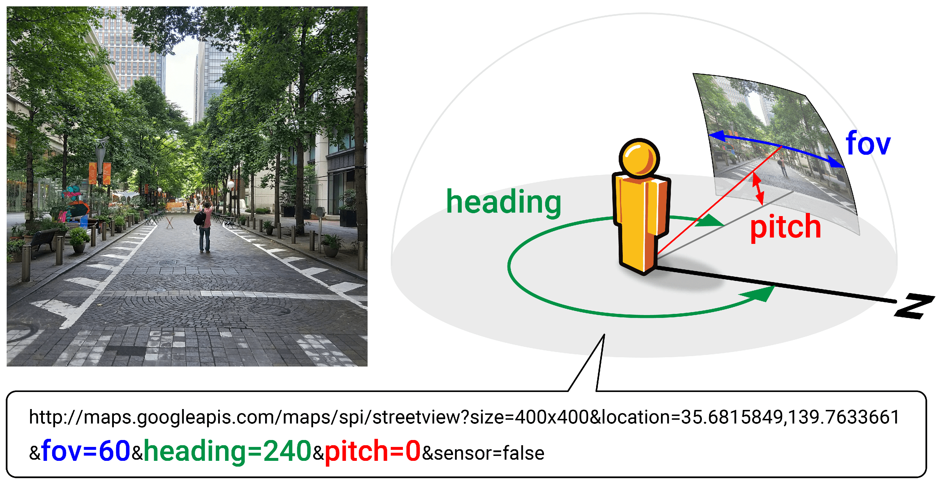
Figure 1 illustrates the process of image retrieval from Google Street View API. At each site, six images with
interval allow to capture all surrounding scenery of the site (
heading), whereas four images with
interval may fail to capture objects at
directions. The vertical view angle (
pitch) is fixed to
, which is parallel to the horizontal line.
Based on the extracted images, the Green View Index (GVI) [
17] is calculated using this formula:
where
n is the number of images for each site, set to six in this study.
is the number of green pixels in the image for
ith direction, and
is the number of total pixels in the image for
ith direction.
Green pixels (
in Equation (
1)) are identified using the spectral information of GSV images [
17]. As green vegetation has high reflection at green band and low reflection at red and blue band, the differences of reflection at each pixel (Green-Red and Green-Blue) are calculated and multiplied themselves. If the product and the differences are positive, the pixel is identified as green pixel. Some previous studies proposed an improved detection methodology with image recognition [
25,
26]; however, the precision of object recognition lies beyond the scope of this study, and we consider the implementation of such advanced techniques future work.
Using metadata collected from the Google Street View API, it is possible to know the months in which the images were taken. Since our interest lies in urban greenery, we defined “green months” for our study area as the period from April to October. Images taken outside of the “green months” are not utilized for analysis.
In addition to limiting images to green months, we implemented the functionality of specifying year of image via the Google Maps JavaScript API [
15]. This allows us to use images of the designated year when available, thus mitigating the bias of temporal fluctuation.
3.2. Standardized Green View Index
GVI is a site-based metric: it measures the visibility of surrounding greenery at a geographical point. However, in practice it is often aggregated to an area level (block, census tract, administrative boundary, etc.), in order to associate the index with other socioeconomic factors. Previous studies [
15,
31] implicitly assumed that each site of GVI calculation has equal importance, hence simply taking the mean of GVI scores of sites located in a given area. However, this assumption may not hold, especially if sites are not evenly distributed in space. A heterogeneous distribution of GVI points will lead to a biased estimation when aggregated to an area level, as points densely located will contribute to the aggregated value to a greater extent.
Figure 2 illustrates an example of such biased estimation. Here, the sites are basically positioned every 100 m, but sites are also added at intersections, because it is plausible that different road segments have different profile of green vegetation, even if the segments are short. Consequently, sites with low GVI are densely located in the upper part of the area, while sites with high GVI are sparsely located in the lower part. Taking the mean of these sites skews the GVI value towards that of the denser parts (upper part of figure), resulting in a biased aggregation at the area-level.
In order to mitigate bias resulting from point density, we propose a Standardized Green View Index (sGVI) to calculate GVI for a given area. The sGVI is a weighted aggregation of GVI scores in a study area. It considers how road segments are located in the area when calculating the area-level value. The idea is to define the expected value of GVI in terms of total road length inside the zone to represent GVI of an area. In other words, sGVI is the expected value of GVI when the site for calculation is randomly chosen on the road network of the area. The mathematical formulation of sGVI is as follows:
where
j is point of GVI calculation
is the total length of links that the point
j is associated with, and
l is the total length of all links in the zone. The association of point
j to links (
) is defined by the Voronoi tessellation of each point: the set of link fragments overlapped by the Voronoi tessellation is associated with point
j. The procedure of this association is illustrated in
Figure 3.
Given a set of sites and an area, the Voronoi tessellation divides the area into cells so that any point in the area belongs to the cell of its closest site. This procedure is implemented using
https://github.com/WZBSocialScienceCenter/geovoronoi of Python. Once the tessellation is defined, the roads are overlapped and cut by each cell. Then the proportion of the road fragments contained in a cell over all the road fragments in the area is calculated, in terms of length of road fragment. These proportions are weighted inversely to the density of sites, which derives from densely located road segments.
One of the advantages of using the Voronoi tessellation over other methods is that every part of the roads is automatically associated with one site, without duplication. Given that the sites for GVI evaluation is located on a road segment, by definition, all the cells in the tessellation are supposed to have at least a fragment of road segment. In addition, since the cells do not overlay each other, it is ensured that one fragment of road segment is associated with only one site. This property may not be the case with other methods based on network configuration: for instance, if one decides to associate a site with nearby road segments, it is possible that two points in different road segments have the same distance from the site. An additional rule of attribution is needed in order to avoid duplicated association. The Voronoi tessellation, in turn, requires only the sites, the road segments and the boundary, and no other parameter is needed. As the Equation (
2) indicates, quasi inverse weighting of GVI sites in terms of site density can be achieved with possibility of simple application in practice.
Validation of this new scheme is presented in
Section 4.
3.3. Normalized Differential Vegetation Index
While the GVI measures visible green vegetation on eye level, the Normalized Differential Vegetation Index (NDVI) quantifies the top-down green coverage using satellite imagery. The NDVI makes use of the fact that green vegetation reflects near-infrared lights more than red lights in the visible spectrum. The formula of NDVI is as follows:
where
is near-infrared light and
is red light. The value is normalized to
, with a larger value signifying more abundant green vegetation.
The images used to calculate NDVI were retrieved from Level-2A data of Sentinel-2 with 10 m resolution via
https://scihub.copernicus.eu. Four images were retrieved for the study period: 9 March, 8 May, 5 August and 6 October 2019, and in order to mitigate seasonal effects, mean values of each image for each pixel were taken. The cloud cover ratio of these images was smaller than 5%.
3.4. Comparison of sGVI and Other Green Metrics
In order to explore the relation between sGVI and other green metrics, the following metrics were calculated in the study area of Yokohama city (see the next section for more detailed description): (1) sGVI, (2) GVI (mean), (3) GVI (median), and (4) NDVI. (1) sGVI is the expected value of GVI in the area, when a site is randomly chosen on the road network of the area. (2) GVI (mean) is an aggregation of GVI in the area by mean [
29,
31], and (3) GVI (median) is an aggregation by median [
15]. (4) NDVI is an aggregation of NDVI in the area by mean. It should be noted that NDVI contains some areas where GVI sites will not be located, since the GVI site is located on street. This may lead to an unfair comparison.
For comparison, correlation among these four indicators is calculated. Then, the pair with the lowest correlation coefficient is further examined in terms of spatial distribution and regression analysis. The calculation of the green metrics was computed on an Intel Core i9 CPU at 2.4 GHz and implemented in Python.
4. Result: Bias Mitigation by sGVI
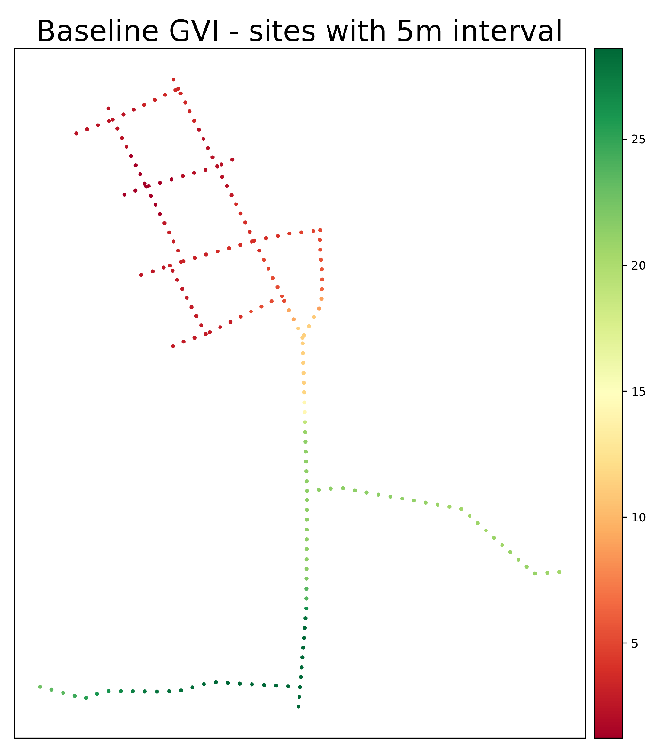
In order to check whether the proposed sGVI mitigates the sampling bias, derived from road density, an experimental comparison on an hypothetical setting is performed. The network (
Figure 4) is the same as that in
Figure 2, but this time the sites are positioned with smaller spatial interval (5 m instead of 100 m). With these quasi-continuous sampling of sites, the mean of GVI for these sites is expected to exclude the bias from site sampling. We consider the mean value as a balanced representation of area-based GVI for this area.
Table 2 provides the result of estimations from different metrics, applied to the network shown in
Figure 2 and
Figure 4. Among the three estimations from sampled sites with 100 m interval, sGVI (calculated with sampled sites with 100 m interval) showed the highest precision compared to the baseline (calculated from the sites with 5 m interval). On the other hand, GVI (mean) and GVI (median) were 28.4% and 69.8% smaller than the baseline respectively. This means that these metrics are biased toward the value where the density of sampled sites is high, although the metrics have often been used in previous studies.
Admittedly, this situation does not occur in every study area, as the difference between mean and median values of GVI depends on the (numerical) distribution of GVI. For instance, if the GVI values in an area follow the normal distribution, the choice between mean and median will be unimportant since the two values are expected to be similar by definition. However, when the distribution is more long-tailed such as power low, the difference between mean and median is not always negligible, and the importance of defining a representative value will increase.
Even if the researcher has complete knowledge of the GVI distribution in the study area (which is divided into sub-areas), it is possible that the distributions that each sub-area follows are not identical. From this viewpoint, a feasible solution to mitigate this bias is to consider the weight of each site depending on their representativeness in the sub-area, which can be realized by sGVI.
The indicator is expected to behave as a proxy of representative value of areas, not only in areas with heterogeneous distribution of sites but also in areas with homogeneous distribution of sites. This is because, with such homogeneously located sites, sGVI leverages each point quasi-equally. If the distribution of GVI of such are is following normal distribution, the estimation by sGVI will be close to the mean and the median of GVI in the area. Such robustness towards distribution of sites and eventual variation of GVI is an advantage of sGVI, which has not been explored in previous studies.
5. Case Study: Yokohama City
While the sGVI was confirmed as a balanced representation of area-based GVI in the previous section, its particularity compared to other green metrics, especially NDVI, must be studied.
5.1. Study Area
The green vegetation metrics defined in the previous section are applied in two wards (Nishi ward and Kanagawa ward) of Yokohama city, Japan. Located South of Tokyo metropolitan region, Yokohama city has its central business district located in the Nishi ward, and peripheral residential areas located in the West part of Kanagawa ward. This city structure allows us to study different behavior of the metrics, depending on the land use pattern. The geographical scale of analysis in this study is at Chome level (the Japanese name for a city block [
33]), since this is the smallest level of division for statistical data in Japan.
The area and population of the study area is shown in
Table A1 in
Appendix A. The locations of the study area is illustrated in
Figure 5 [
34].
5.2. Descriptive Analysis
This section describes basic statistics of the data source that is used, namely GVI from Google Street View imagery and NDVI from satellite imagery.
For GVI, 7780 sites are selected in total, and six corresponding images per site are retrieved via the Google Street View API. The sites are located every 100 m along a link in the road network, and it is ensured that intersections have at least one site (if images satisfying criteria of season and year are available). 84% of the sites turned out to have images taken in 2019 (see
Figure 6). This mitigates the time fluctuation, which has been pointed out in previous studies [
17,
32]. Furthermore, the month of image taking is limited to the period from April to October, with the majority (83%) of images being taken in April or May.
As for NDVI, four satellite images are retrieved and the mean value for each mesh was calculated. In contrast to GVI, this aggregation will not produce spatial bias, because every satellite image has the same spatial resolution. The study area has in total 307,335 (70,273 (Nishi) + 237,062 (Kanagawa)) meshes with 10 m spatial resolution.
Figure A1 in
Appendix A illustrates the geographical distribution of NDVI.
Figure 7 shows the histograms of NDVI and GVI for the study area, and the descriptive information is shown in
Table 3.
5.3. Comparison of Different Green Metrics
In order to further understand characteristics of the suggested indicator, sGVI, we first analyze the statistical relation between sGVI and NDVI. In this analysis, the Chome zones where sGVI is 0 are excluded. This is because of either lack of available image on Google Street View or absence of streets. With this pre-processed data set, Spearman’s rank correlation between the two metrics was calculated (
Table 4), and the result was 0.72 (
p ≪ 0.01). It should be noted that Pearson’s correlation is not appropriate here because the distributions of sGVI and NDVI do not follow normal distribution, which is a prerequisite for performing Pearson’s correlation test.
Figure 8 illustrates the scatter plot of sGVI and NDVI as well as the regressed line of NDVI by sGVI at Chome level. The coefficient of determination was 0.55. From this result, we see that factors other than sGVI contribute to more than 40% of the fluctuation of NDVI. Similar results were observed between GVI and NDVI in previous studies [
18,
32]. This brings the question of what these other influencing factors are.
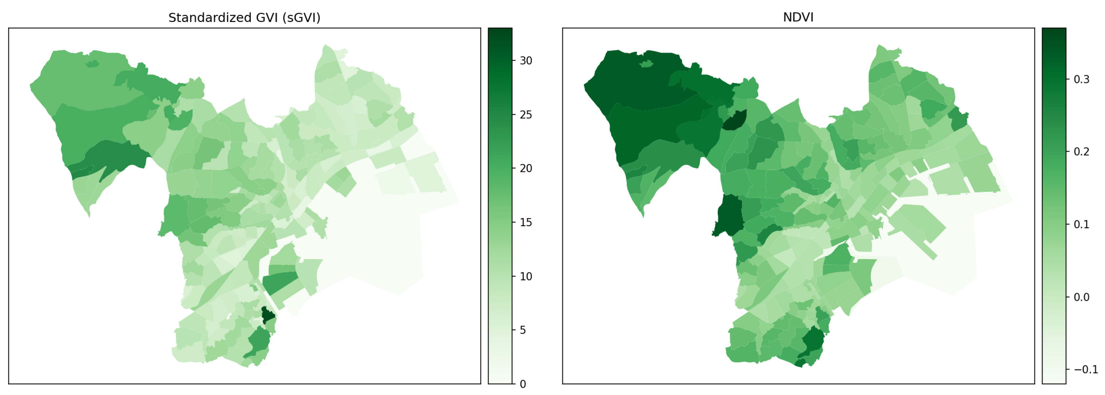
In the aim of exploring the above question, second, the geographical distribution of the estimated values was explored.
Figure 9 visually compares sGVI and NDVI calculated at Chome level. Even though the scales of value between sGVI and NDVI are not directly comparable, there is an observable tendency that NDVI leverages the vegetation in the north-west part of the study area.
Spatial distribution of residual error from the regression analysis is also illustrated in
Figure 10. Under an assumption that the relation between sGVI and NDVI can be modeled by a linear function, NDVI in the north-west part where vegetation is more present is larger than what sGVI predicts, and NDVI in the south-east part where buildings are more dominant is smaller than the prediction by sGVI.
Given that the north-west part is mainly a residential area with parks and gardens, and that the south-east part is the central business district with limited number of vegetation along streets, this result indicates that sGVI captures the green vegetation in urbanized area more than NDVI. In other words, presence of buildings makes it difficult to estimate the amount of green vegetation from the top-down viewpoint.
6. Discussion
6.1. Spatial Aggregation of Weighted Points
In geography, “everything is related to everything else, but near things are more related than distant things” [
35]. Spatial distribution of objects must therefore be considered when arguing at spatial level. From this viewpoint, simple aggregation of GVI values in a given area by mean signifies that every site is assumed to be related equally to every other sites, which is clearly false. If two sites are close, the images taken in the two sites are likely to capture an identical tree, whereas two distant sites do not have anything in common in their images. It is thus necessary to consider the spatial proximity of each site in order to estimate green vegetation, not for a site (point), but for a certain area.
This study proposed standardized GVI (sGVI), which is able to consider the heterogeneous relation among sites. Explicitly considering physical existence of road network, sGVI can mitigate a biased estimation caused by simply aggregating the mean value.
It is also possible to imagine other possibilities of weighting, especially using tools of spatial statistics. For instance, smoothing techniques such as Kernel Density Estimation (KDE) may be an option. However, KDE normally leverages densely located sites by definition, whereas the problem of aggregating GVI over an area is the opposite: provide less weight to densely located sites. This is why this method is not introduced in this study, but it may be a possible direction for future study.
6.2. Different Perspective: NDVI and GVI Groups
It has been pointed out that NDVI and GVI capture different aspects of green vegetation, due to their different viewpoints.
NDVI has a top-down viewpoint due to its use of satellite imagery, which makes it possible to capture horizontal extension of green vegetation better than other perspectives. Knowing that vegetation grows in a way that gives leaves maximum sunlight, it is reasonable to represent the existence of vegetation by NDVI. Nevertheless, it should be noted that there is green vegetation on building walls, especially in the city center, which is not fully captured by NDVI.
On the other hand, GVI has a street-level viewpoint. This is closer to humans’ perception, but has several limitations. First, vegetation hindered by objects are not considered. Second, the estimation of GVI is limited on streets where pavement necessarily appears in the images, thus lowering the estimated value. Third, canopy formed by tall trees may be only partially perceived by people on the street, since the canopy will be placed at the marge of the eyesight, which is fixed in the horizontal direction. Lastly, densely located sites may be auto-correlated, because the same tree may be observed more than once, especially if the sites are very closely located.
These points themselves are consistent with the standpoint that GVI measures the visibility of urban green vegetation, but will lead inconsistency when GVI is employed as a proxy of the existence of vegetation. The usage of indicators deriving from GVI (including sGVI), thus, should be limited to measure visibility of green vegetation.
6.3. Insight for Further Analytical Work
Multiple green vegetation metrics have been proposed, some of which are treated in this study. However, differences among them have not been fully understood. The result of this study, namely the comparison of NDVI and GVI, implies that the innate characteristic of each metric must be more carefully considered when associated with other factors.
Taking an example of physiological study, green vegetation is expected to have positive effects on physical health outcomes [
18]. Nevertheless, when the causal relation between presence of green vegetation and health outcomes, there will be at least two paths: one is optical, and the other is atmospheric/olfactory/bacterial. The former corresponds to the effect of just “seeing“ greenery, whereas the latter corresponds to the effect of more direct interaction between human body and vegetation, such as quality of air, smell of plants and presence of certain bacteria. It is clear that GVI and FGVI [
28] is an appropriate method to measure the former, while NDVI is more suitable to evaluate the latter.
For statistical analysis, attention must also be paid to the aggregation method. Presence of several mediators between green vegetation and physiological outcome has been remarked [
36], but spatial aggregation of site-based metrics has not been discussed. The proposed method of sGVI mitigates the bias from heterogeneous distribution of measurement points of GVI.
Association with these green vegetation metrics and other factors must be carefully discussed, knowing the properties of each method.
7. Conclusions
People’s exposure to green vegetation is often associated with social, economic or physiological factors, but it has been overlooked that aggregation method of green metrics may generate bias in area-based estimation. This study implemented GVI [
17] with development of designating time of image shooting, and proposed a new metric, standardized GVI (sGVI), which considers the density of sites for GVI calculation. We found that sGVI mitigates such density-led bias, and expect increased robustness to heterogeneous spatial distribution of sites compared to a simple aggregation by mean or median. Furthermore, it was shown that NDVI, which is derived from satellite images and has a top-down viewpoint, leverages green vegetation in residential area with parks and gardens, while sGVI captures more vegetation in urban area where buildings are dominant. Therefore, for further analyses associating green vegetation and other factors, especially in urban areas, it is recommended to employ sGVI since it mitigates bias from spatial distribution of sites and captures eye-level greenery in a more sensitive manner than NDVI.
For future work, there are two major issues to be considered. Firstly, the heavy computational load of Voronoi tessellation, especially when calculating sGVI in a large area, is not ideal. Keeping the idea of leveraging sparsely located sites, another direction with a lighter computational load must be explored.
The second issue is the treatment of missing points when estimating sGVI. Since not every site has images that satisfy the given conditions such as month and year, robustness to missing points must be considered in greater detail. While it is possible to mitigate this by placing sites with smaller intervals (20 m instead of 100 m, for example), it is not cost-efficient both in terms of time and money, since Google Street View API is not free: users are billed by the number of images requested via the API.
Under the SARS-CoV-2 epidemic, reduction of social contact by taking distance between people has been requested. Such situation may increase the importance of spaces outside buildings, and, thus, understanding the roles of the components in the outdoor space is crucial. Moreover, as trees are expected to play a critical role in sustainable development in environmental terms as well as in terms of public health, quantification of green space at wide range is important. From these viewpoints, sGVI prepares a solid foundation on association studies, which will contribute to the design of public space in the context of sustainable development.
Author Contributions
Conceptualization, Y.K. and Y.Y.; methodology, Y.K., S.Y.C. and Y.Y.; software, Y.K., S.Y.C. and X.L.; validation, Y.K.; formal analysis, Y.K.; investigation, Y.K.; resources, Y.K., S.Y.C. and X.L.; data curation, Y.K. and S.Y.C.; writing—original draft preparation, Y.K.; writing—review and editing, S.Y.C., H.K., X.L. and Y.Y.; visualization, Y.K.; supervision, Y.Y.; project administration, Y.Y.; funding acquisition, Y.Y. All authors have read and agreed to the published version of the manuscript.
Funding
This research received no external funding.
Conflicts of Interest
The authors declare no conflict of interest.
Abbreviations
The following abbreviations are used in this manuscript:
| GVI | Green View Index |
| GSV | Google Street View |
| sGVI | Standardized Green View Index |
| NDVI | Normalized Difference Vegetation Index |
Appendix A. Miscellaneous Information About the Study Area
Table A1.
Statistics of the study area (1 January 2020).
Table A1.
Statistics of the study area (1 January 2020).
| | Area [km] | Household | Population |
|---|
| Nishi | 6.98 | 55,811 | 103,985 |
| Kanagawa | 23.59 | 126,093 | 245,036 |
Figure A1.
NDVI in the study area.
Figure A1.
NDVI in the study area.
References
- United Nations. World Urbanization Prospects—The 2018 Revision; Technical Report; Department of Economic and Social Affairs, United Nations: New York, NY, USA, 2018. [Google Scholar]
- Wakefield, S.E.; Elliott, S.J.; Cole, D.C.; Eyles, J.D. Environmental risk and (re) action: Air quality, health, and civic involvement in an urban industrial neighbourhood. Health Place 2001, 7, 163–177. [Google Scholar] [CrossRef]
- Livesley, S.; McPherson, E.; Calfapietra, C. The urban forest and ecosystem services: Impacts on urban water, heat, and pollution cycles at the tree, street, and city scale. J. Environ. Qual. 2016, 45, 119–124. [Google Scholar] [CrossRef] [PubMed]
- Janhäll, S. Review on urban vegetation and particle air pollution—Deposition and dispersion. Atmos. Environ. 2015, 105, 130–137. [Google Scholar] [CrossRef]
- Norton, B.A.; Coutts, A.M.; Livesley, S.J.; Harris, R.J.; Hunter, A.M.; Williams, N.S. Planning for cooler cities: A framework to prioritise green infrastructure to mitigate high temperatures in urban landscapes. Landsc. Urban Plan. 2015, 134, 127–138. [Google Scholar] [CrossRef]
- Sanusi, R.; Johnstone, D.; May, P.; Livesley, S.J. Microclimate benefits that different street tree species provide to sidewalk pedestrians relate to differences in Plant Area Index. Landsc. Urban Plan. 2017, 157, 502–511. [Google Scholar] [CrossRef]
- Tzoulas, K.; Korpela, K.; Venn, S.; Yli-Pelkonen, V.; Kaźmierczak, A.; Niemela, J.; James, P. Promoting ecosystem and human health in urban areas using Green Infrastructure: A literature review. Landsc. Urban Plan. 2007, 81, 167–178. [Google Scholar] [CrossRef]
- Lee, A.C.; Maheswaran, R. The health benefits of urban green spaces: A review of the evidence. J. Public Health 2011, 33, 212–222. [Google Scholar] [CrossRef]
- Jesdale, B.M.; Morello-Frosch, R.; Cushing, L. The racial/ethnic distribution of heat risk–related land cover in relation to residential segregation. Environ. Health Perspect. 2013, 121, 811–817. [Google Scholar] [CrossRef]
- Nutsford, D.; Pearson, A.; Kingham, S. An ecological study investigating the association between access to urban green space and mental health. Public Health 2013, 127, 1005–1011. [Google Scholar] [CrossRef]
- Astell-Burt, T.; Feng, X. Association of urban green space with mental health and general health among adults in Australia. JAMA Netw. Open 2019, 2, e198209. [Google Scholar] [CrossRef]
- Turner-Skoff, J.B.; Cavender, N. The benefits of trees for livable and sustainable communities. Plants People Planet 2019, 1, 323–335. [Google Scholar] [CrossRef]
- Wolch, J.R.; Byrne, J.; Newell, J.P. Urban green space, public health, and environmental justice: The challenge of making cities ‘just green enough’. Landsc. Urban Plan. 2014, 125, 234–244. [Google Scholar] [CrossRef]
- Boone, C.G.; Buckley, G.L.; Grove, J.M.; Sister, C. Parks and People: An Environmental Justice Inquiry in Baltimore, Maryland. Ann. Assoc. Am. Geogr. 2009, 99, 767–787. [Google Scholar] [CrossRef]
- Li, X.; Zhang, C.; Li, W.; Kuzovkina, Y.A. Environmental inequities in terms of different types of urban greenery in Hartford, Connecticut. Urban For. Urban Green. 2016, 18, 163–172. [Google Scholar] [CrossRef]
- Gerrish, E.; Watkins, S.L. The relationship between urban forests and income: A meta-analysis. Landsc. Urban Plan. 2018, 170, 293–308. [Google Scholar] [CrossRef]
- Li, X.; Zhang, C.; Li, W.; Ricard, R.; Meng, Q.; Zhang, W. Assessing street-level urban greenery using Google Street View and a modified green view index. Urban For. Urban Green. 2015, 14, 675–685. [Google Scholar] [CrossRef]
- Larkin, A.; Hystad, P. Evaluating street view exposure measures of visible green space for health research. J. Expo. Sci. Environ. Epidemiol. 2019, 29, 447–456. [Google Scholar] [CrossRef]
- Yang, J.; Zhao, L.; Mcbride, J.; Gong, P. Can you see green? Assessing the visibility of urban forests in cities. Landsc. Urban Plan. 2009, 91, 97–104. [Google Scholar] [CrossRef]
- Li, X.; Zhang, C.; Li, W.; Kuzovkina, Y.A.; Weiner, D. Who lives in greener neighborhoods? The distribution of street greenery and its association with residents’ socioeconomic conditions in Hartford, Connecticut, USA. Urban For. Urban Green. 2015, 14, 751–759. [Google Scholar] [CrossRef]
- Villeneuve, P.J.; Ysseldyk, R.L.; Root, A.; Ambrose, S.; DiMuzio, J.; Kumar, N.; Shehata, M.; Xi, M.; Seed, E.; Li, X.; et al. Comparing the normalized difference vegetation index with the Google Street view measure of vegetation to assess associations between greenness, walkability, recreational physical activity, and health in Ottawa, Canada. Int. J. Environ. Res. Public Health 2018, 15, 1719. [Google Scholar] [CrossRef]
- Lu, Y. Using Google Street View to investigate the association between street greenery and physical activity. Landsc. Urban Plan. 2019, 191, 103435. [Google Scholar] [CrossRef]
- James, P.; Banay, R.F.; Hart, J.E.; Laden, F. A review of the health benefits of greenness. Curr. Epidemiol. Rep. 2015, 2, 131–142. [Google Scholar] [CrossRef] [PubMed]
- Gascon, M.; Cirach, M.; Martínez, D.; Dadvand, P.; Valentín, A.; Plasència, A.; Nieuwenhuijsen, M.J. Normalized difference vegetation index (NDVI) as a marker of surrounding greenness in epidemiological studies: The case of Barcelona city. Urban For. Urban Green. 2016, 19, 88–94. [Google Scholar] [CrossRef]
- Cai, B.Y.; Li, X.; Seiferling, I.; Ratti, C. Treepedia 2.0: Applying deep learning for large-scale quantification of urban tree cover. In Proceedings of the 2018 IEEE International Congress on Big Data (BigData Congress), Seattle, WA, USA, 10–13 December 2018; pp. 49–56. [Google Scholar]
- Cai, B.; Li, X.; Ratti, C. Quantifying Urban Canopy Cover with Deep Convolutional Neural Networks. arXiv 2019, arXiv:1912.02109. [Google Scholar]
- Chen, X.; Meng, Q.; Hu, D.; Zhang, L.; Yang, J. Evaluating greenery around streets using baidu panoramic street view images and the panoramic green view index. Forests 2019, 10, 1109. [Google Scholar] [CrossRef]
- Yu, S.; Yu, B.; Song, W.; Wu, B.; Zhou, J.; Huang, Y.; Wu, J.; Zhao, F.; Mao, W. View-based greenery: A three-dimensional assessment of city buildings’ green visibility using floor green view index. Landsc. Urban Plan. 2016, 152, 13–26. [Google Scholar] [CrossRef]
- Li, X.; Ghosh, D. Associations between body mass index and urban “green” streetscape in Cleveland, Ohio, USA. Int. J. Environ. Res. Public Health 2018, 15, 2186. [Google Scholar] [CrossRef]
- Helbich, M.; Yao, Y.; Liu, Y.; Zhang, J.; Liu, P.; Wang, R. Using deep learning to examine street view green and blue spaces and their associations with geriatric depression in Beijing, China. Environ. Int. 2019, 126, 107–117. [Google Scholar] [CrossRef]
- Lu, Y.; Sarkar, C.; Xiao, Y. The effect of street-level greenery on walking behavior: Evidence from Hong Kong. Soc. Sci. Med. 2018, 208, 41–49. [Google Scholar] [CrossRef]
- Ye, Y.; Richards, D.; Lu, Y.; Song, X.; Zhuang, Y.; Zeng, W.; Zhong, T. Measuring daily accessed street greenery: A human-scale approach for informing better urban planning practices. Landsc. Urban Plan. 2019, 191, 103434. [Google Scholar] [CrossRef]
- Gao, X.; Asami, Y. Effect of urban landscapes on land prices in two Japanese cities. Landsc. Urban Plan. 2007, 81, 155–166. [Google Scholar] [CrossRef]
- Yokohama City. Yokohama City Statistic GIS Data. 2020. Available online: https://www.city.yokohama.lg.jp/city-info/seisaku/torikumi/shien/gis/tokei-gis/gistat.html (accessed on 1 August 2020).
- Tobler, W.R. A computer movie simulating urban growth in the Detroit region. Econ. Geogr. 1970, 46, 234–240. [Google Scholar] [CrossRef]
- Wang, R.; Helbich, M.; Yao, Y.; Zhang, J.; Liu, P.; Yuan, Y.; Liu, Y. Urban greenery and mental wellbeing in adults: Cross-sectional mediation analyses on multiple pathways across different greenery measures. Environ. Res. 2019, 176, 108535. [Google Scholar] [CrossRef] [PubMed]
© 2020 by the authors. Licensee MDPI, Basel, Switzerland. This article is an open access article distributed under the terms and conditions of the Creative Commons Attribution (CC BY) license (http://creativecommons.org/licenses/by/4.0/).


