An Elitist Multi-Objective Particle Swarm Optimization Algorithm for Sustainable Dynamic Economic Emission Dispatch Integrating Wind Farms


Abstract
1. Introduction
1.1. Research Background
1.2. Related Works
1.3. Aims and Contributions
2. Materials and Methods
2.1. Chance-Constrained DEED Problem
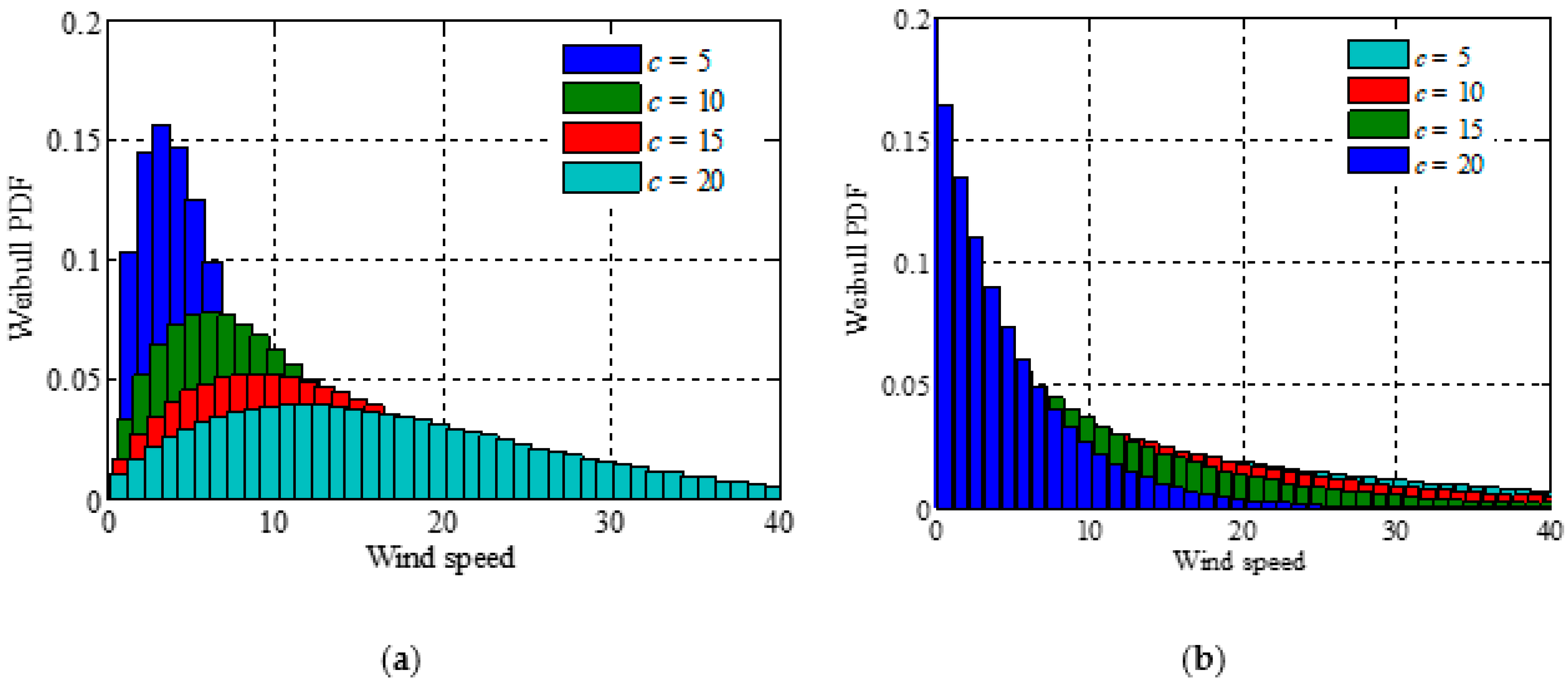
2.2. Probability Model of WP Output
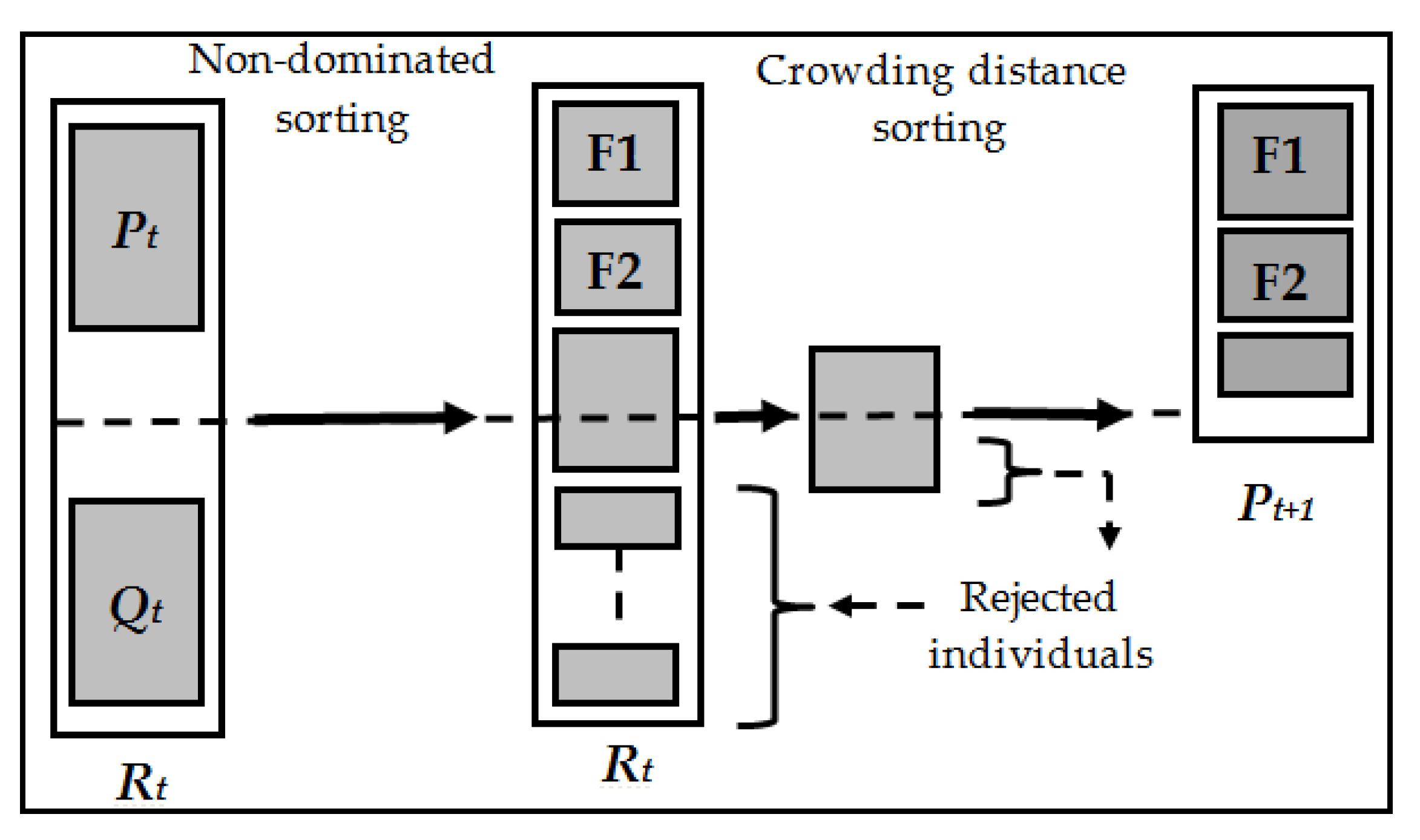
2.3. Implementation of the Non-Dominated Sorting PSO Algorithm
3. Results and Discussion
- (i)
- SEED problem without wind power.
- (ii)
- DEED problem without wind power.
- (iii)
- DEED problem with wind power.
3.1. Case 1: SEED Problem without Wind Power
3.2. Case 2: DEED Problem without Wind Power
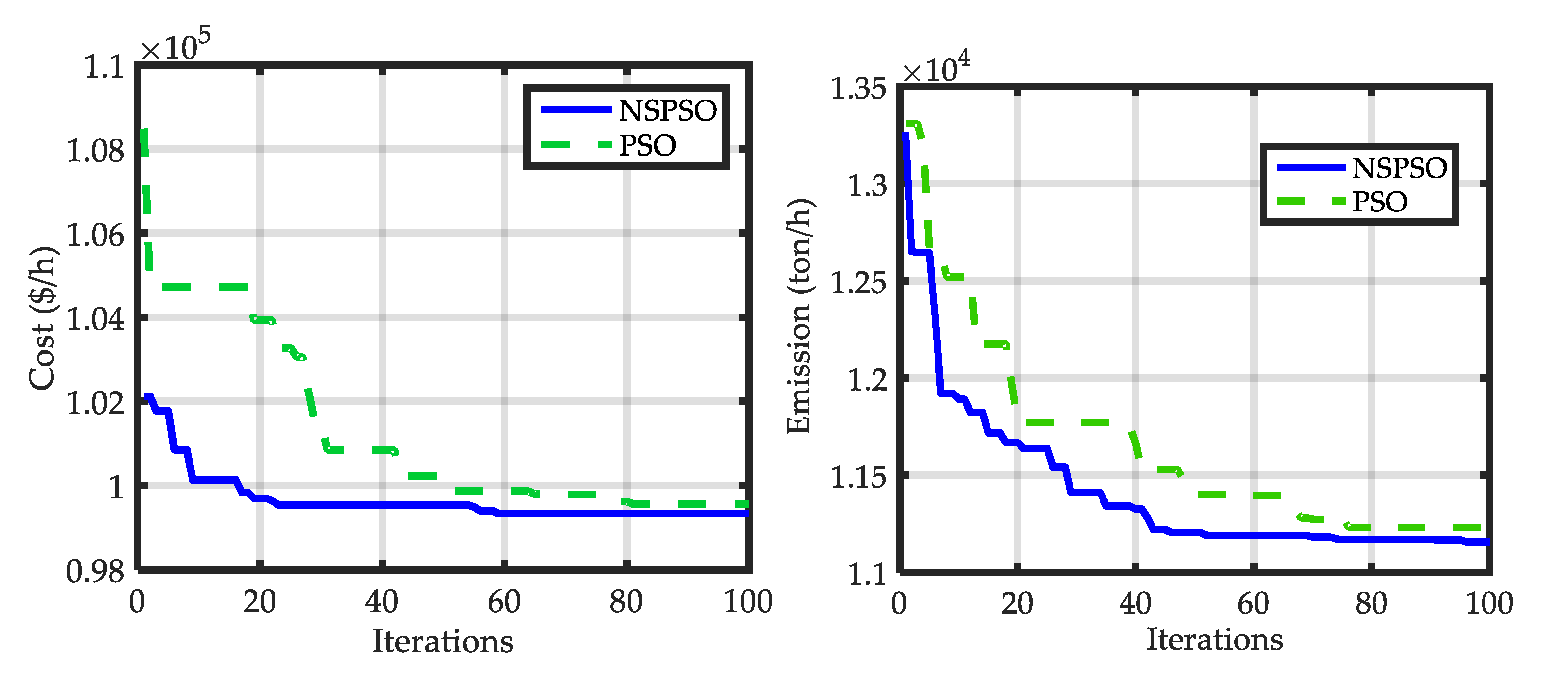
3.3. Case 3: DEED with Wind Power
4. Conclusions
Author Contributions
Funding
Acknowledgments
Conflicts of Interest
Nomenclature
| CT | Total fuel cost in USD |
| ET | Total emission in ton |
| N: | Number of thermal units |
| ai, bi, ci, di and ei | Cost coefficients |
| αi, βi, γi, ηi, and λI | Emission coefficients |
| Generation in MW of unit i at time t | |
| Total demand power in MW at time t | |
| Probability of event | |
| α | Probability that the energy balance constraint cannot be met |
| Wind power output at time t | |
| Total losses in MW at time t | |
| N | Number of thermal units |
| and | Minimum and maximum limits of generation of unit i, respectively |
| and | Down-ramp and up-ramp limits of the of the i-th unit in MW |
| and | Down and up limits of the k-th POZ of unit i, respectively |
| Number of POZ for the i-th unit | |
| Probability density function (PDF) | |
| Cumulative distribution function (CDF) | |
| v | Wind speed in m/s |
| V and PW | Wind speed and wind power random variables |
| k and c | Shape and scale factors of the Weibull distribution function, respectively |
| , and | Cut-in, cut-out and rated wind speeds in m/s, respectively |
| wr | Rated wind power output in MW |
Appendix A

| Unit | ai | bi | ci | di | ei | αi | βi | γi | ηi | λi |
|---|---|---|---|---|---|---|---|---|---|---|
| 1 | 786.7988 | 38.5397 | 0.1524 | 450 | 0.041 | 103.3908 | −2.4444 | 0.0312 | 0.5035 | 0.0207 |
| 2 | 451.3251 | 46.1591 | 0.1058 | 600 | 0.036 | 103.3908 | −2.4444 | 0.0312 | 0.5035 | 0.0207 |
| 3 | 1049.9977 | 40.3965 | 0.0280 | 320 | 0.028 | 300.3910 | −4.0695 | 0.0509 | 0.4968 | 0.0202 |
| 4 | 1243.5311 | 38.3055 | 0.0354 | 260 | 0.052 | 300.3910 | −4.0695 | 0.0509 | 0.4968 | 0.0202 |
| 5 | 1658.5696 | 36.3278 | 0.0211 | 280 | 0.063 | 320.0006 | −3.8132 | 0.0344 | 0.4972 | 0.0200 |
| 6 | 1356.6592 | 38.2704 | 0.0179 | 310 | 0.048 | 320.0006 | −3.8132 | 0.0344 | 0.4972 | 0.0200 |
| 7 | 1450.7045 | 36.5104 | 0.0121 | 300 | 0.086 | 330.0056 | −3.9023 | 0.0465 | 0.5163 | 0.0214 |
| 8 | 1450.7045 | 36.5104 | 0.0121 | 340 | 0.082 | 330.0056 | −3.9023 | 0.0465 | 0.5163 | 0.0214 |
| 9 | 1455.6056 | 39.5804 | 0.1090 | 270 | 0.098 | 350.0056 | −3.9524 | 0.0465 | 0.5475 | 0.0234 |
| 10 | 1469.4026 | 40.5407 | 0.1295 | 380 | 0.094 | 360.0012 | −3.9864 | 0.0470 | 0.5475 | 0.0234 |
| Unit | ||||
|---|---|---|---|---|
| 1 | 150 | 470 | 80 | 80 |
| 2 | 135 | 470 | 80 | 80 |
| 3 | 73 | 340 | 80 | 80 |
| 4 | 60 | 300 | 50 | 50 |
| 5 | 73 | 243 | 50 | 50 |
| 6 | 57 | 160 | 50 | 50 |
| 7 | 20 | 130 | 30 | 30 |
| 8 | 47 | 120 | 30 | 30 |
| 9 | 20 | 80 | 30 | 30 |
| 10 | 10 | 55 | 30 | 30 |
| Hour | 1 | 2 | 3 | 4 | 5 | 6 | 7 | 8 | 9 | 10 | 11 | 12 |
|---|---|---|---|---|---|---|---|---|---|---|---|---|
| Load (MW) | 1036 | 1110 | 1258 | 1406 | 1480 | 1628 | 1702 | 1776 | 1924 | 2022 | 2106 | 2150 |
| Hour | 13 | 14 | 15 | 16 | 17 | 18 | 19 | 20 | 21 | 22 | 23 | 24 |
| Load (MW) | 2072 | 1924 | 1776 | 1554 | 1480 | 1628 | 1776 | 1972 | 1924 | 1628 | 1332 | 1184 |
| Units | Best Cost | Best Emission | ||
|---|---|---|---|---|
| NSPSO | PSO | NSPSO | PSO | |
| 1 | 113.9975 | 113.6956 | 444.5290 | 439.2442 |
| 2 | 111.2700 | 108.5791 | 118.8684 | 118.8350 |
| 3 | 97.7987 | 97.5901 | 119.5250 | 119.1685 |
| 4 | 78.6822 | 180.8286 | 120.0000 | 120.0000 |
| 5 | 87.7614 | 89.4804 | 171.0041 | 171.3165 |
| 6 | 39.3092 | 135.9100 | 99.6506 | 100.0000 |
| 7 | 61.0281 | 262.3170 | 126.4088 | 123.6008 |
| 8 | 84.7192 | 286.7468 | 293.3165 | 293.0055 |
| 9 | 282.9047 | 289.1561 | 298.0365 | 298.3546 |
| 10 | 129.1357 | 128.6181 | 296.4214 | 297.2705 |
| 11 | 165.2336 | 165.0649 | 136.1537 | 137.1096 |
| 12 | 94.1237 | 95.2535 | 298.0555 | 298.7171 |
| 13 | 125.0462 | 127.4267 | 300.0000 | 299.9239 |
| 14 | 393.5936 | 393.9443 | 435.5130 | 437.5409 |
| 15 | 304.3556 | 303.7451 | 428.8594 | 428.4812 |
| 16 | 395.9528 | 392.3604 | 424.3950 | 425.0628 |
| 17 | 489.8036 | 486.7798 | 418.5687 | 420.6127 |
| 18 | 489.6818 | 480.9941 | 438.3276 | 438.2479 |
| 19 | 512.0610 | 517.3487 | 441.5894 | 443.2781 |
| 20 | 512.6642 | 511.1498 | 437.8936 | 436.2938 |
| 21 | 523.1834 | 523.5155 | 433.7515 | 434.5389 |
| 22 | 523.1455 | 532.7049 | 432.6224 | 431.5904 |
| 23 | 521.7535 | 536.3904 | 432.0455 | 431.4084 |
| 24 | 523.5970 | 528.3499 | 437.9027 | 439.7005 |
| 25 | 525.0606 | 523.1002 | 433.8896 | 434.0663 |
| 26 | 535.5420 | 546.2872 | 437.0916 | 435.3730 |
| 27 | 11.6919 | 13.9834 | 440.2194 | 439.3075 |
| 28 | 10.0623 | 18.6982 | 28.2081 | 27.6326 |
| 29 | 10.0201 | 13.3795 | 28.3884 | 27.9565 |
| 30 | 95.7998 | 83.7703 | 28.3276 | 30.0000 |
| 31 | 199.9715 | 182.6645 | 98.9027 | 99.7623 |
| 32 | 200.0000 | 196.3166 | 171.4707 | 170.4029 |
| 33 | 200.0000 | 199.0675 | 171.9558 | 171.7829 |
| 34 | 203.7138 | 186.6948 | 169.5057 | 169.1000 |
| 35 | 170.1866 | 181.6321 | 200.0000 | 200.0000 |
| 36 | 202.3923 | 195.0869 | 200.0000 | 199.8316 |
| 37 | 120.0000 | 119.0675 | 200.0000 | 199.9375 |
| 38 | 113.7251 | 114.3643 | 102.1179 | 103.9197 |
| 39 | 120.0000 | 108.4289 | 103.8253 | 103.8042 |
| 40 | 521.0316 | 529.5086 | 102.6590 | 103.8210 |
| Cost (USD/h) | 121,153 | 122,362 | 129,911 | 129,945 |
| Emission (USD/h) | 389,953 | 4.10112 | 176,299 | 176,305 |
References
- Pandit, N.; Tripathi, A.; Tapaswi, S.; Pandit, M. An improved bacterial foraging algorithm for combined static/dynamic environmental economic dispatch. Appl. Soft Comput. 2012, 12, 3500–3513. [Google Scholar] [CrossRef]
- Huang, W.T.; Yao, K.; Chen, M.K.; Wang, F.Y.; Zhu, C.H.; Chang, Y.R.; Lee, Y.D.; Ho, Y.H. Derivation and Application of a New Transmission Loss Formula for Power System Economic Dispatch. Energies 2018, 11, 417. [Google Scholar] [CrossRef]
- Hazra, S.; Roy, P.K. Quasi-oppositional chemical reaction optimization for combined economic emission dispatch in power system considering wind power uncertainties. Renew. Energy Focus 2019, 31, 45–62. [Google Scholar] [CrossRef]
- Liang, Z.; Glover, J.D. A zoom feature for a dynamic programming solution to economic dispatch including transmission losses. IEEE Trans. Power Syst. 1992, 7, 544–550. [Google Scholar] [CrossRef]
- Gar, M.C.W.; Aganagic, J.G.; Meding, T.; Jose, B.; Reeves, S. Experience with mixed integer linear programming based approach on short term hydrothermal scheduling. IEEE Trans. Power Syst. 2001, 16, 743–749. [Google Scholar]
- Torres, G.; Quintana, V. On a nonlinear multiple centrality corrections interior-point method for optimal power flow. IEEE Trans. Power Syst. 2001, 16, 222–228. [Google Scholar] [CrossRef]
- Ganjefar, S.; Tofighi, M. Dynamic economic dispatch solution using an improved genetic algorithm with non-stationary penalty functions. Eur. Trans. Electr. Power 2011, 21, 1480–1492. [Google Scholar] [CrossRef]
- Lu, H.; Sriyanyong, P.; Song, Y.H.; Dillon, T. Experimental Study of a New Hybrid PSO with Mutation for Economic Dispatch with Non-smooth Cost Function. Int. J. Electr. Power 2010, 32, 921–935. [Google Scholar] [CrossRef]
- Sen, T.; Mathur, H.D. A new approach to solve Economic Dispatch problem using a Hybrid ACO–ABC–HS optimization algorithm. Int. J. Electr. Power 2016, 78, 735–744. [Google Scholar] [CrossRef]
- Vaisakh, K.; Praveena, P.; Naga Sujatha, K. Solution of Dynamic Economic Emission Dispatch Problem by Hybrid Bacterial Foraging Algorithm. Int. J. Comput. Sci. Electron. Eng. 2014, 2, 58–64. [Google Scholar]
- Niknam, T.; Narimani, M.R.; Jabbari, M. Dynamic optimal power flow using hybrid particle swarm optimization and simulated annealing. Int. Trans. Electr. Energy Syst. 2013, 23, 975–1001. [Google Scholar] [CrossRef]
- Jiang, X.; Zhou, J.; Wang, H.; Zhang, Y. Dynamic environmental economic dispatch using multiobjective differential evolution algorithm with expanded double selection and adaptive random restart. Int. J. Electr. Power 2013, 49, 399–407. [Google Scholar] [CrossRef]
- Hetzer, J.; Yu, C.D.; Bhattarai, K. An economic dispatch model incorporating wind power. IEEE Trans. Energy Convers. 2008, 23, 603–611. [Google Scholar] [CrossRef]
- Liu, X.; Xu, W. Economic load dispatch constrained by wind power availability: A here-and-now approach. IEEE Trans. Sustain. Energy 2010, 1, 1–9. [Google Scholar] [CrossRef]
- Roy, P.K.; Bhui, S. Multi-objective quasi-oppositional teaching learning based optimization for economic emission load dispatch problem. Int. J. Electr. Power 2013, 53, 937–948. [Google Scholar] [CrossRef]
- Zhu, Y.; Wang, J.; Qu, B. Multi-objective economic emission dispatch considering wind power using evolutionary algorithm based on decomposition. Int. J. Electr. Power 2014, 63, 434–445. [Google Scholar] [CrossRef]
- Alham, M.H.; Elshahed, M.; Ibrahim, D.K.; Abo El Zahab, E.E.D. A dynamic economic emission dispatch considering wind power uncertainty incorporating energy storage system and demand side management. Renew. Energy 2016, 96, 800–811. [Google Scholar] [CrossRef]
- Hu, Y.; Li, Y.; Xu, M.; Zhou, L.; Cui, M. A Chance-Constrained Economic Dispatch Model in Wind-Thermal-Energy Storage System. Energies 2017, 10, 326. [Google Scholar] [CrossRef]
- Teeparthi, K.; Vinod Kumar, D.M. Multi-objective hybrid PSO-APO algorithm based security constrained optimal power flow with wind and thermal generators. Eng. Sci. Technol. 2017, 20, 411–426. [Google Scholar] [CrossRef]
- Aghaei, J.; Niknam, T.; Azizipanah-Abarghooee, R.; Arroyo, J.M. Scenario-based dynamic economic emission dispatch considering load and wind power uncertainties. Int. J. Electr. Power 2013, 47, 351–367. [Google Scholar] [CrossRef]
- Biswas, P.; Suganthan, P.N.; Mallipeddi, R.; Amaratunga, G.A.J. Optimal reactive power dispatch with uncertainties in load demand and renewable energy sources adopting scenario-based approach. Appl. Soft Comput. 2019, 75, 616–632. [Google Scholar] [CrossRef]
- Jadhav, H.T.; Roy, R. Gbest guided artificial bee colony algorithm for environmental/economic dispatch considering wind power. Exp. Syst. Appl. 2013, 40, 6385–6399. [Google Scholar] [CrossRef]
- Zou, D.; Li, S.; Li, Z.; Kong, X. A new global particle swarm optimization for the economic emission dispatch with or without transmission losses. Energy Convers. Manag. 2017, 139, 45–70. [Google Scholar] [CrossRef]
- Hagh, M.T.; Kalajahi, S.M.S.; Ghorbani, N. Solution to economic emission dispatch problem including wind farms using Exchange Market Algorithm Method. Appl. Soft Comput. 2020, 88, 1–10. [Google Scholar] [CrossRef]
- Liu, G.; Zhu, Y.; Jang, W. Wind-thermal dynamic economic emission dispatch with a hybrid multi-objective algorithm based on wind speed statistical analysis. IET Gener. Transm. Dis. 2018, 12, 3972–3984. [Google Scholar] [CrossRef]
- Kennedy, J.; Eberhart, R. Particle swarm optimization. In Proceedings of the IEEE International Conference on Neural Networks 1995, Perth, Australia, 27 November–1 December 1995; pp. 1942–1948. [Google Scholar]
- Rezaei, F.; Safavi, H.R.; Mirchi, A.; Madani, K. f-MOPSO: An alternative multi-objective PSO algorithm for conjunctive water use management. J. Hydro Environ. Res. 2017, 14, 1–18. [Google Scholar] [CrossRef]
- Deb, K.; Pratap, A.; Agarwal, S.; Meyarivan, T. A fast and elitist multiobjective genetic algorithm: NSGA-II. Trans. Evol. Comput. 2002, 6, 182–197. [Google Scholar] [CrossRef]
- Kien, L.C.; Duong, T.L.; Phan, V.D.; Nguyen, T.T. Maximizing Total Profit of Thermal Generation Units in Competitive Electric Market by Using a Proposed Particle Swarm Optimization. Sustainability 2020, 12, 1265. [Google Scholar] [CrossRef]
- Mahmoud, K.; Abdel-Nasser, M.; Mustafa, E.; Ali, Z.M. Improved Salp—Swarm Optimizer and Accurate Forecasting Model for Dynamic Economic Dispatch in Sustainable Power Systems. Sustainability 2020, 12, 576. [Google Scholar] [CrossRef]


| Techniques | Dispatch Problems |
|---|---|
| Dynamic programming [4] | Static economic dispatch problem without valve-point loading effects (VPLE) constraints |
| Interior point method [6] | Nonlinear optimal power flow |
| Particle swarm optimization (PSO) [8] | Static economic dispatch with VPLE constraints |
| Artificial bee colony (ABC) [9] | |
| Genetic algorithm [7] | Dynamic economic dispatch problem with VPLE constraints |
| Bacterial foraging [10] | Dynamic economic emission dispatch (DEED) problem with VPLE constraints |
| Simulated annealing [11] | |
| Differential evolution (DE) [12] | |
| Here-and-now approach [14] | Static economic dispatch problem including wind power and without VPLE |
| Stochastic optimization technique [15] | Static economic emission dispatch (SEED) problem considering wind power |
| Chance-constraint programming [16] | SEED problem considering wind power |
| Chance-constraint programming [17] | DEED problem considering wind power |
| Chance-constraint programming [18] | Static economic dispatch considering wind power and without VPLE |
| Scenario-based approach [20] | DEED problem considering wind power |
| Scenario-based approach [21] | Reactive power dispatch considering renewable energy sources and with uncertainties in loads. |
| Method | Minimum Total Cost (USD) | Minimum Total Emission (ton) |
|---|---|---|
| NSPSO | 2,474,472.8 | 293,416.3 |
| PSO | 2,491,480.2 | 2.97696 |
| IBFA [1] | 2,481,733.3 | 295,833.0 |
| NSGAII [2] | 2.5168 × 10⁶ | 3.1740 × 10⁵ |
| Hour | P1 | P2 | P3 | P4 | P5 | P6 | P7 | P8 | P9 | P10 | WP |
|---|---|---|---|---|---|---|---|---|---|---|---|
| 1 | 152.19 | 135.00 | 143.75 | 60.00 | 73.00 | 160.00 | 130.00 | 98.50 | 25.23 | 46.13 | 30.89 |
| 2 | 150.07 | 137.64 | 191.51 | 60.00 | 121.47 | 152.07 | 130.00 | 120.00 | 20.00 | 16.13 | 32.42 |
| 3 | 152.45 | 135.00 | 271.51 | 110.00 | 171.47 | 145.20 | 130.00 | 120.00 | 20.00 | 12.62 | 17.80 |
| 4 | 154.32 | 135.00 | 268.30 | 145.34 | 217.31 | 155.92 | 123.12 | 119.74 | 50.00 | 39.69 | 31.44 |
| 5 | 153.35 | 136.00 | 297.97 | 168.14 | 227.50 | 160.00 | 130.00 | 118.81 | 49.26 | 44.39 | 32.52 |
| 6 | 196.18 | 135.00 | 329.35 | 218.14 | 243.00 | 144.52 | 130.00 | 120.00 | 71.22 | 55.00 | 32.33 |
| 7 | 151.82 | 199.68 | 340.00 | 255.06 | 237.69 | 160.00 | 123.16 | 120.00 | 80.00 | 55.00 | 30.84 |
| 8 | 166.04 | 226.41 | 340.00 | 300.00 | 243.00 | 160.00 | 130.00 | 120.00 | 80.00 | 53.27 | 14.60 |
| 9 | 224.73 | 306.41 | 340.00 | 300.00 | 243.00 | 160.00 | 130.00 | 120.00 | 80.00 | 55.00 | 32.63 |
| 10 | 252.51 | 386.41 | 340.00 | 300.00 | 243.00 | 160.00 | 130.00 | 120.00 | 80.00 | 54.27 | 32.46 |
| 11 | 272.99 | 466.41 | 340.00 | 300.00 | 243.00 | 160.00 | 130.00 | 120.00 | 80.00 | 46.38 | 32.33 |
| 12 | 308.76 | 470.00 | 340.00 | 300.00 | 243.00 | 160.00 | 130.00 | 120.00 | 80.00 | 55.00 | 32.49 |
| 13 | 272.91 | 463.03 | 327.97 | 300.00 | 232.48 | 160.00 | 130.00 | 103.97 | 79.81 | 55.00 | 29.48 |
| 14 | 195.22 | 383.58 | 311.62 | 300.00 | 243.00 | 159.38 | 129.81 | 119.01 | 76.49 | 42.81 | 31.80 |
| 15 | 152.33 | 303.58 | 301.25 | 300.00 | 243.00 | 129.41 | 130.00 | 120.00 | 78.15 | 44.18 | 31.32 |
| 16 | 161.55 | 223.58 | 221.25 | 250.00 | 233.79 | 160.00 | 130.00 | 120.00 | 55.00 | 14.18 | 27.29 |
| 17 | 150.68 | 145.58 | 218.55 | 239.01 | 243.00 | 144.51 | 129.86 | 119.07 | 51.30 | 44.18 | 32.04 |
| 18 | 151.05 | 213.33 | 297.55 | 249.74 | 232.67 | 154.08 | 126.38 | 117.79 | 54.29 | 45.89 | 31.88 |
| 19 | 178.47 | 293.33 | 300.00 | 299.74 | 243.00 | 160.00 | 130.00 | 87.79 | 53.17 | 55.00 | 32.57 |
| 20 | 212.61 | 373.33 | 340.00 | 300.00 | 243.00 | 160.00 | 130.00 | 117.79 | 80.00 | 55.00 | 32.50 |
| 21 | 231.14 | 308.96 | 339.73 | 299.43 | 243.00 | 160.00 | 125.76 | 119.94 | 76.99 | 54.78 | 32.20 |
| 22 | 152.08 | 232.02 | 262.12 | 249.43 | 239.68 | 160.00 | 130.00 | 120.00 | 52.59 | 44.88 | 31.91 |
| 23 | 153.27 | 152.02 | 182.12 | 235.39 | 189.68 | 110.00 | 100.00 | 120.00 | 80.00 | 14.88 | 25.64 |
| 24 | 152.08 | 135.00 | 117.01 | 185.39 | 156.80 | 100.04 | 130.00 | 90.00 | 80.00 | 31.39 | 30.48 |
| Cost (USD) | 2,433,467.20 | ||||||||||
| Emission (ton) | 331,251.40 | ||||||||||
| Hour | P1 | P2 | P3 | P4 | P5 | P6 | P7 | P8 | P9 | P10 | WP |
|---|---|---|---|---|---|---|---|---|---|---|---|
| 1 | 165.58 | 135.60 | 88.56 | 73.46 | 133.09 | 119.92 | 92.78 | 92.31 | 78.23 | 54.01 | 21.60 |
| 2 | 165.52 | 136.28 | 95.30 | 91.47 | 136.97 | 132.32 | 100.62 | 116.64 | 79.97 | 55.00 | 21.75 |
| 3 | 165.70 | 157.99 | 115.67 | 117.19 | 163.79 | 159.98 | 129.38 | 119.54 | 79.96 | 54.98 | 21.76 |
| 4 | 195.69 | 197.85 | 138.87 | 139.11 | 203.33 | 160.00 | 130.00 | 120.00 | 80.00 | 54.95 | 21.69 |
| 5 | 216.08 | 213.04 | 149.59 | 155.70 | 219.00 | 160.00 | 129.69 | 120.00 | 79.93 | 55.00 | 21.62 |
| 6 | 245.43 | 250.33 | 182.85 | 189.66 | 242.54 | 159.60 | 129.70 | 119.86 | 79.89 | 55.00 | 21.76 |
| 7 | 265.32 | 270.48 | 202.15 | 209.58 | 241.34 | 160.00 | 130.00 | 120.00 | 80.00 | 55.00 | 21.73 |
| 8 | 284.88 | 287.09 | 225.55 | 227.96 | 242.92 | 160.00 | 129.76 | 119.96 | 79.97 | 55.00 | 21.71 |
| 9 | 326.49 | 317.64 | 268.44 | 277.96 | 243.00 | 157.18 | 130.00 | 120.00 | 80.00 | 54.67 | 18.91 |
| 10 | 340.26 | 355.82 | 340.00 | 268.08 | 243.00 | 160.00 | 130.00 | 120.00 | 80.00 | 51.92 | 11.95 |
| 11 | 384.79 | 366.58 | 340.00 | 300.00 | 243.00 | 160.00 | 130.00 | 120.00 | 78.17 | 55.00 | 14.91 |
| 12 | 394.93 | 395.50 | 340.00 | 300.00 | 243.00 | 160.00 | 130.00 | 120.00 | 80.00 | 55.00 | 21.77 |
| 13 | 356.63 | 356.77 | 332.55 | 299.30 | 242.81 | 159.97 | 129.92 | 120.00 | 79.87 | 54.87 | 21.76 |
| 14 | 323.38 | 324.57 | 265.26 | 272.00 | 242.98 | 159.96 | 129.66 | 119.67 | 79.89 | 55.00 | 21.76 |
| 15 | 287.40 | 287.15 | 224.63 | 226.75 | 243.00 | 160.00 | 129.69 | 119.79 | 79.84 | 55.00 | 21.61 |
| 16 | 234.54 | 235.52 | 170.56 | 176.75 | 238.93 | 160.00 | 130.00 | 120.00 | 55.00 | 55.00 | 21.75 |
| 17 | 218.58 | 217.50 | 160.73 | 158.17 | 224.54 | 159.47 | 129.03 | 119.99 | 54.93 | 55.00 | 21.71 |
| 18 | 253.80 | 256.98 | 191.47 | 190.38 | 242.58 | 159.98 | 130.00 | 120.00 | 54.89 | 55.00 | 21.69 |
| 19 | 293.70 | 291.55 | 231.14 | 234.04 | 243.00 | 159.96 | 129.96 | 119.98 | 54.95 | 54.95 | 21.73 |
| 20 | 301.23 | 340.24 | 311.14 | 284.04 | 243.00 | 160.00 | 130.00 | 120.00 | 80.00 | 55.00 | 20.92 |
| 21 | 322.36 | 316.67 | 269.77 | 275.90 | 242.94 | 159.92 | 130.00 | 119.88 | 79.79 | 54.99 | 21.76 |
| 22 | 244.56 | 236.67 | 189.77 | 225.90 | 243.00 | 160.00 | 100.00 | 120.00 | 80.00 | 55.00 | 21.62 |
| 23 | 165.11 | 157.07 | 109.77 | 175.90 | 193.00 | 160.00 | 125.62 | 120.00 | 80.00 | 55.00 | 21.75 |
| 24 | 170.50 | 137.02 | 116.29 | 125.90 | 143.00 | 148.23 | 107.99 | 104.65 | 80.00 | 55.00 | 20.17 |
| Cost (USD) | 2,552,118.86 | ||||||||||
| Emission (ton) | 283,538.16 | ||||||||||
| Hour | P1 | P2 | P3 | P4 | P5 | P6 | P7 | P8 | P9 | P10 | WP |
|---|---|---|---|---|---|---|---|---|---|---|---|
| 1 | 150.11 | 135.64 | 77.13 | 113.31 | 123.76 | 125.26 | 94.02 | 86.25 | 64.89 | 52.62 | 31.51 |
| 2 | 150.13 | 135.00 | 83.51 | 110.89 | 167.96 | 128.21 | 95.09 | 94.21 | 78.68 | 55.00 | 32.57 |
| 3 | 151.74 | 138.19 | 130.19 | 125.09 | 172.81 | 159.16 | 124.66 | 119.95 | 76.13 | 55.00 | 32.23 |
| 4 | 155.27 | 144.41 | 176.07 | 172.92 | 222.81 | 154.32 | 130.00 | 120.00 | 80.00 | 55.00 | 29.37 |
| 5 | 166.61 | 189.98 | 188.18 | 184.09 | 219.69 | 159.73 | 128.33 | 119.41 | 80.00 | 49.56 | 32.59 |
| 6 | 208.48 | 220.78 | 203.56 | 225.51 | 243.00 | 159.56 | 128.76 | 119.74 | 80.00 | 53.65 | 32.10 |
| 7 | 255.24 | 245.79 | 220.35 | 275.51 | 243.00 | 129.32 | 130.00 | 89.74 | 80.00 | 55.00 | 30.94 |
| 8 | 220.71 | 300.02 | 277.02 | 269.20 | 243.00 | 157.83 | 100.00 | 119.74 | 80.00 | 37.67 | 28.59 |
| 9 | 274.93 | 289.02 | 326.95 | 294.78 | 243.00 | 155.08 | 129.49 | 117.97 | 80.00 | 48.61 | 32.35 |
| 10 | 298.85 | 369.02 | 310.79 | 300.00 | 243.00 | 160.00 | 130.00 | 120.00 | 80.00 | 55.00 | 32.26 |
| 11 | 287.06 | 449.02 | 340.00 | 300.00 | 243.00 | 160.00 | 130.00 | 120.00 | 80.00 | 55.00 | 27.25 |
| 12 | 338.40 | 463.32 | 334.81 | 297.73 | 239.12 | 157.06 | 128.35 | 118.05 | 77.85 | 54.55 | 30.57 |
| 13 | 312.20 | 383.32 | 340.00 | 300.00 | 243.00 | 159.68 | 129.85 | 120.00 | 79.20 | 53.61 | 32.44 |
| 14 | 274.94 | 310.29 | 295.01 | 293.28 | 242.08 | 159.90 | 130.00 | 119.61 | 80.00 | 54.76 | 32.49 |
| 15 | 225.34 | 250.11 | 288.03 | 262.93 | 242.66 | 160.00 | 121.27 | 119.74 | 80.00 | 53.24 | 29.71 |
| 16 | 150.21 | 203.99 | 251.89 | 232.77 | 228.27 | 153.00 | 126.88 | 116.35 | 51.72 | 55.00 | 26.48 |
| 17 | 159.48 | 168.06 | 203.71 | 195.09 | 243.00 | 160.00 | 129.39 | 116.88 | 55.00 | 55.00 | 32.33 |
| 18 | 210.39 | 236.26 | 241.82 | 243.83 | 232.79 | 153.36 | 130.00 | 86.88 | 55.00 | 54.52 | 30.67 |
| 19 | 248.46 | 249.38 | 264.83 | 293.83 | 243.00 | 160.00 | 130.00 | 110.55 | 55.00 | 55.00 | 23.65 |
| 20 | 290.34 | 310.01 | 340.00 | 293.29 | 243.00 | 157.66 | 130.00 | 120.00 | 74.49 | 55.00 | 30.54 |
| 21 | 285.72 | 296.94 | 302.19 | 293.47 | 242.59 | 159.99 | 130.00 | 119.57 | 79.11 | 54.62 | 28.42 |
| 22 | 213.06 | 223.41 | 222.19 | 243.47 | 213.47 | 160.00 | 129.62 | 117.53 | 80.00 | 41.53 | 30.95 |
| 23 | 156.28 | 143.41 | 184.23 | 193.47 | 163.47 | 160.00 | 99.62 | 120.00 | 80.00 | 37.35 | 24.93 |
| 24 | 151.87 | 135.00 | 115.93 | 145.17 | 182.97 | 133.97 | 129.62 | 90.00 | 50.00 | 43.52 | 30.02 |
| Cost (USD) | 2,466,582.70 | ||||||||||
| Emission (ton) | 298,159.46 | ||||||||||
| α | Dynamic Economic Dispatch | Dynamic Emission Dispatch | Compromise Solution | |||
|---|---|---|---|---|---|---|
| Cost (×106 (USD)) | Emission (×105 ton) | Cost (×106 (USD)) | Emission (×105 ton) | Cost (×106 (USD)) | Emission (×105 ton) | |
| 0.25 | 2.433467 | 3.31251 | 2.552118 | 2.83538 | 2.466582 | 2.98159 |
| 0.3 | 2.376280 | 3.07791 | 2.506736 | 2.70929 | 2.427758 | 2.80227 |
| 0.35 | 2.360207 | 3.02358 | 2.470134 | 2.65313 | 2.394421 | 2.72884 |
| Ratio η | 5% | 10% | 15% | 20% |
| Cost (USD/h) | 83,865 | 82,007 | 80,312 | 78,579 |
| Emission (ton/h) | 7570 | 7190 | 6818 | 6481 |
© 2020 by the authors. Licensee MDPI, Basel, Switzerland. This article is an open access article distributed under the terms and conditions of the Creative Commons Attribution (CC BY) license (http://creativecommons.org/licenses/by/4.0/).
Share and Cite
Alshammari, M.E.; Ramli, M.A.M.; Mehedi, I.M. An Elitist Multi-Objective Particle Swarm Optimization Algorithm for Sustainable Dynamic Economic Emission Dispatch Integrating Wind Farms. Sustainability 2020, 12, 7253. https://doi.org/10.3390/su12187253
Alshammari ME, Ramli MAM, Mehedi IM. An Elitist Multi-Objective Particle Swarm Optimization Algorithm for Sustainable Dynamic Economic Emission Dispatch Integrating Wind Farms. Sustainability. 2020; 12(18):7253. https://doi.org/10.3390/su12187253
Chicago/Turabian StyleAlshammari, Motaeb Eid, Makbul A. M. Ramli, and Ibrahim M. Mehedi. 2020. "An Elitist Multi-Objective Particle Swarm Optimization Algorithm for Sustainable Dynamic Economic Emission Dispatch Integrating Wind Farms" Sustainability 12, no. 18: 7253. https://doi.org/10.3390/su12187253
APA StyleAlshammari, M. E., Ramli, M. A. M., & Mehedi, I. M. (2020). An Elitist Multi-Objective Particle Swarm Optimization Algorithm for Sustainable Dynamic Economic Emission Dispatch Integrating Wind Farms. Sustainability, 12(18), 7253. https://doi.org/10.3390/su12187253