Assessing Impacts of Land Use/Land Cover Conversion on Changes in Ecosystem Services Value on the Loess Plateau, China


Abstract
1. Introduction
2. Materials and Methods
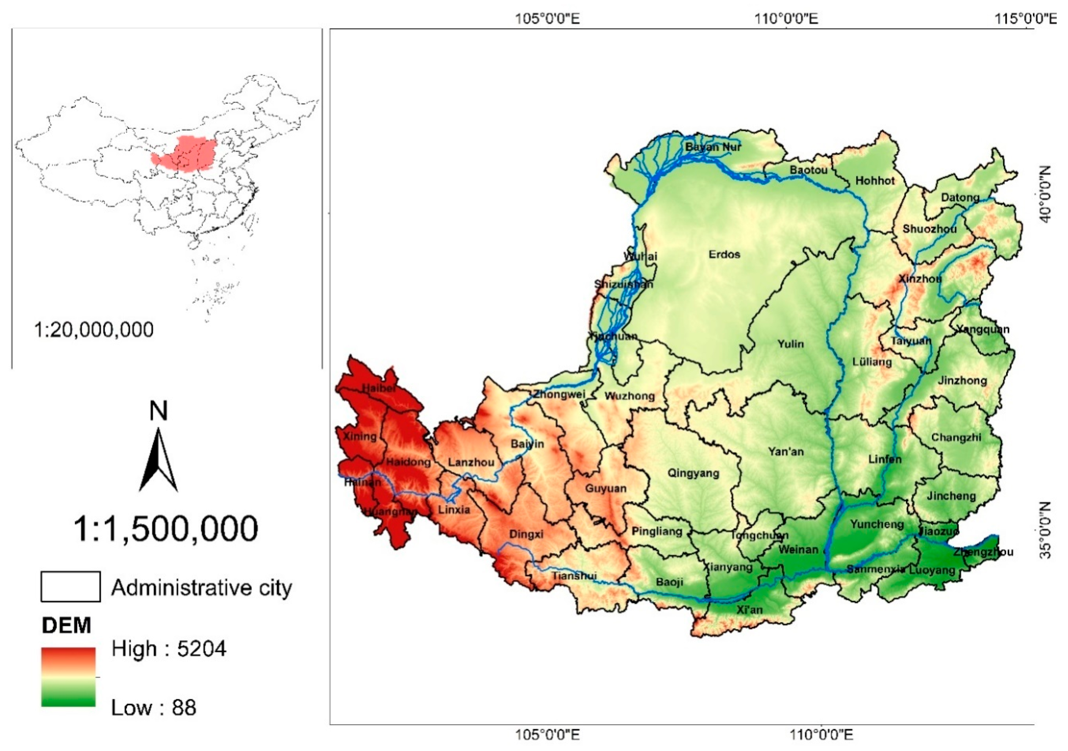
2.1. Study Area
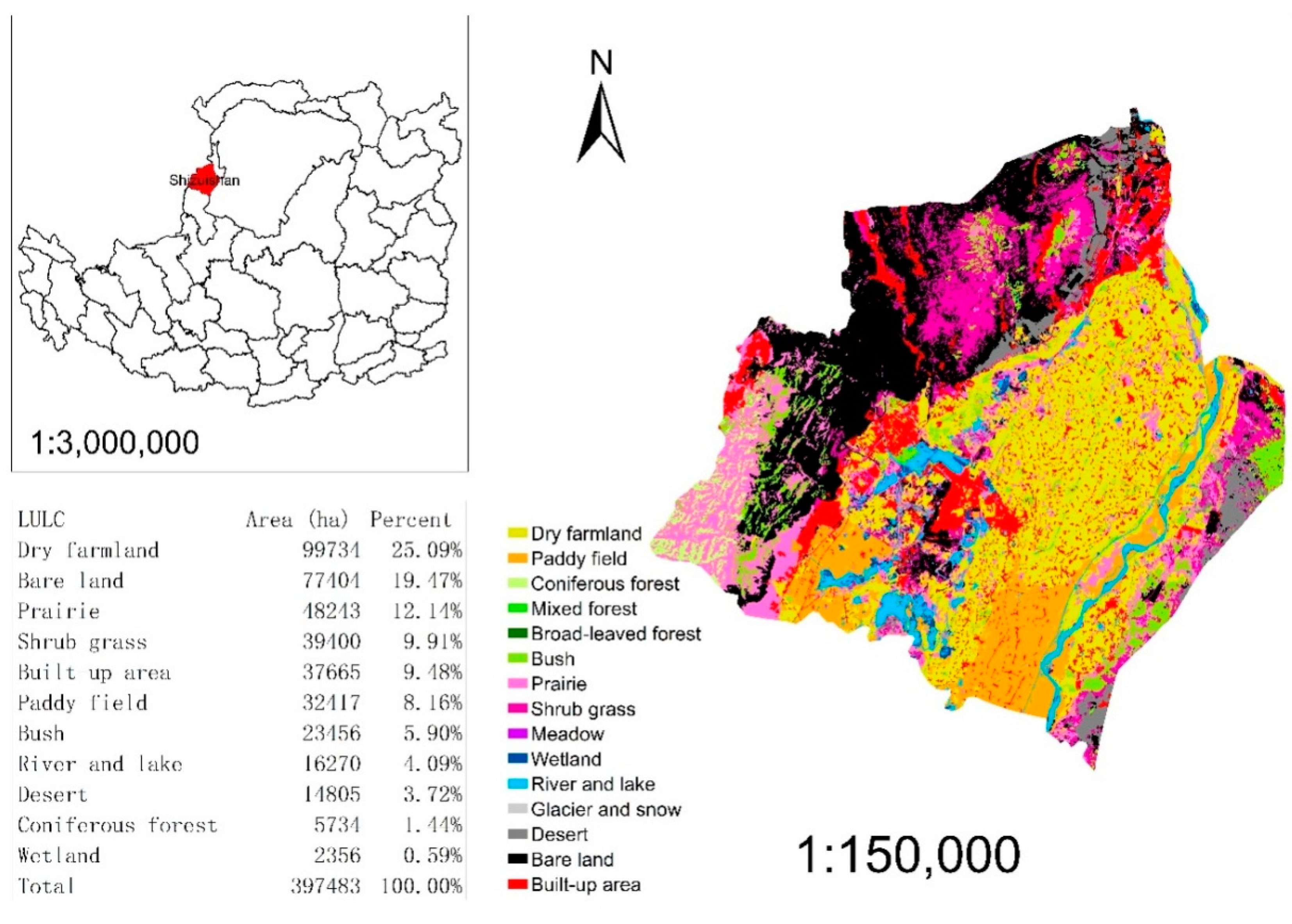
2.2. Identifying LULC
2.3. Calculating ESVs
2.4. Analyzing Elasticity of ESV Changes in Response to LULC Changes
3. Results
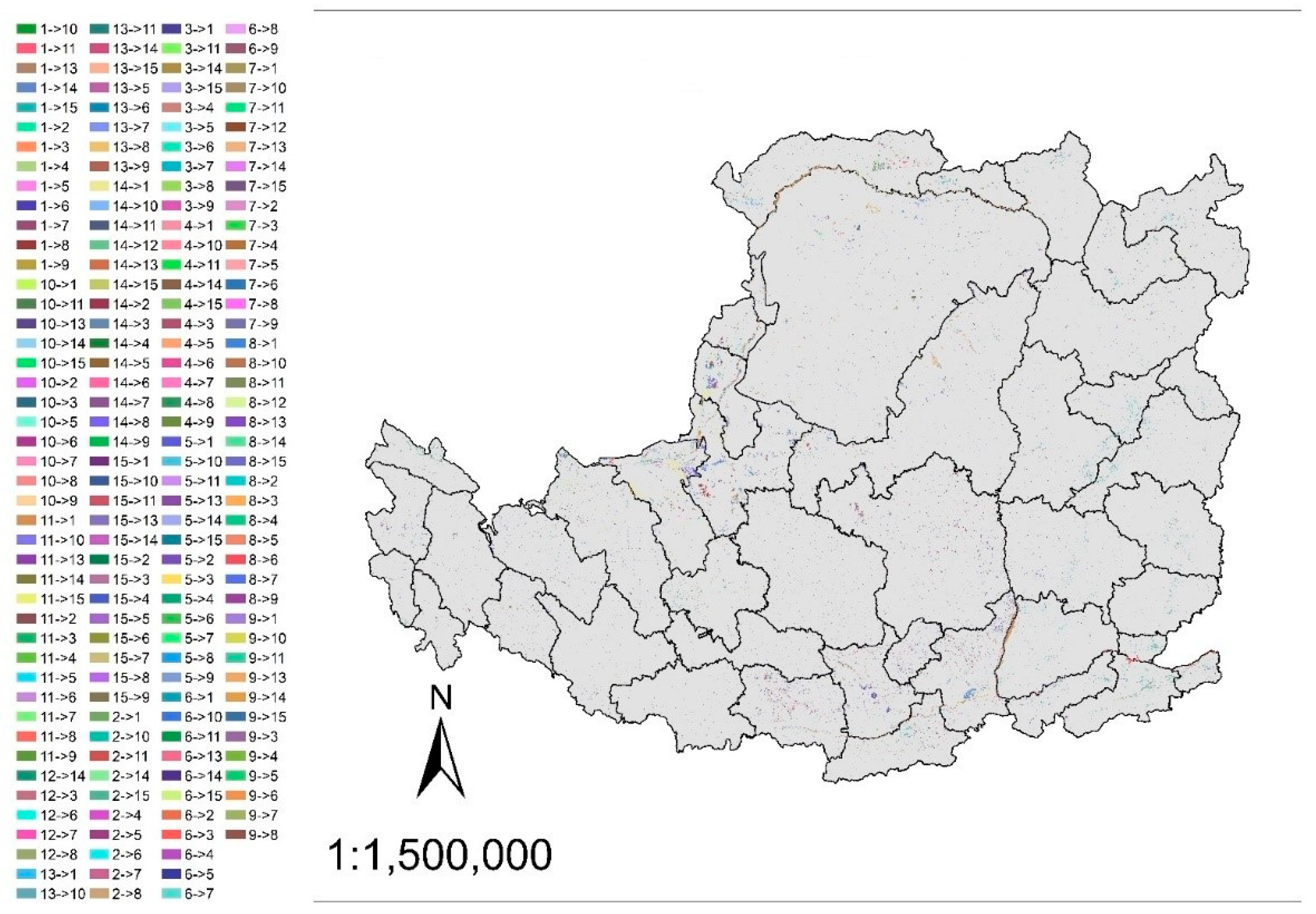
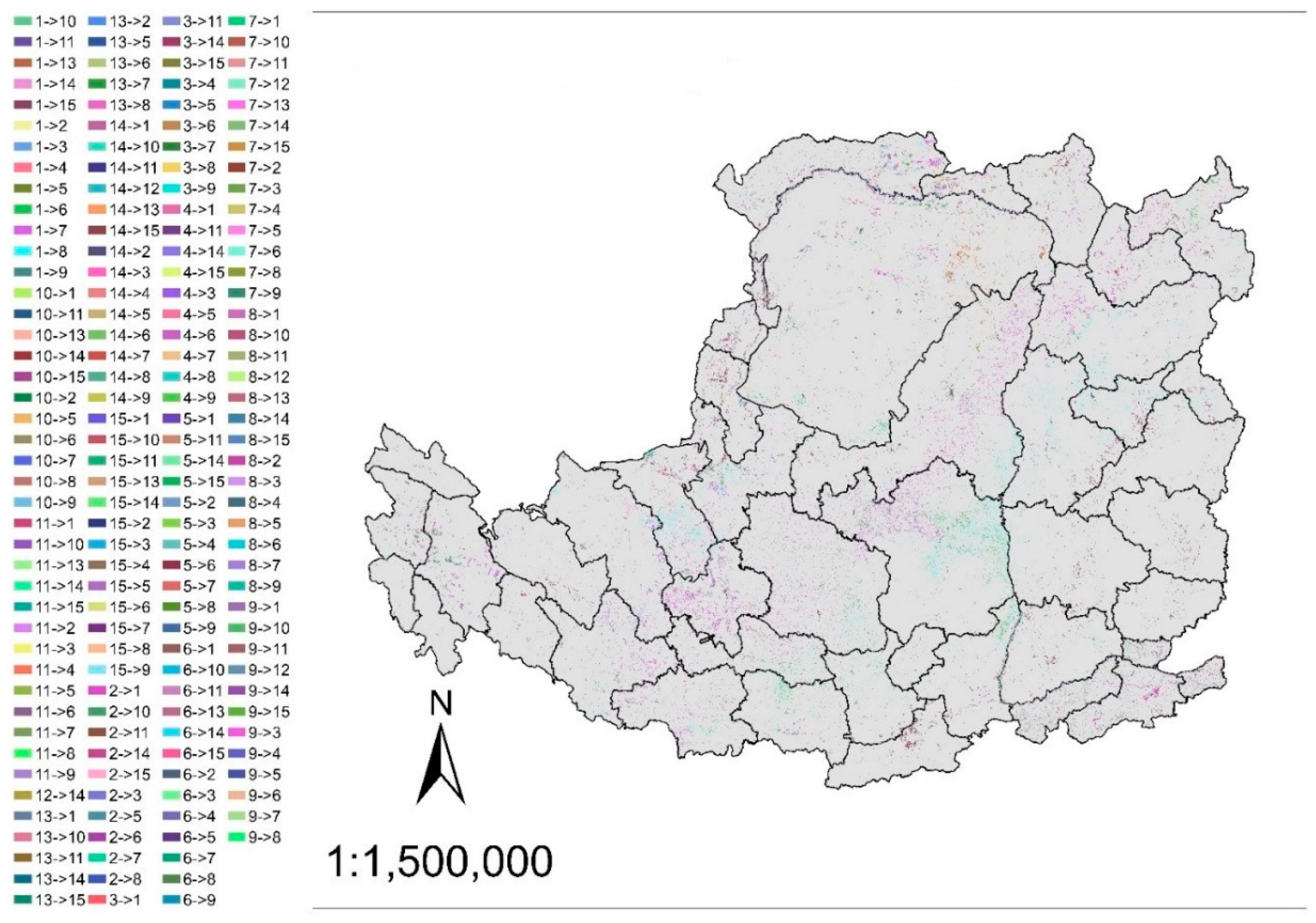
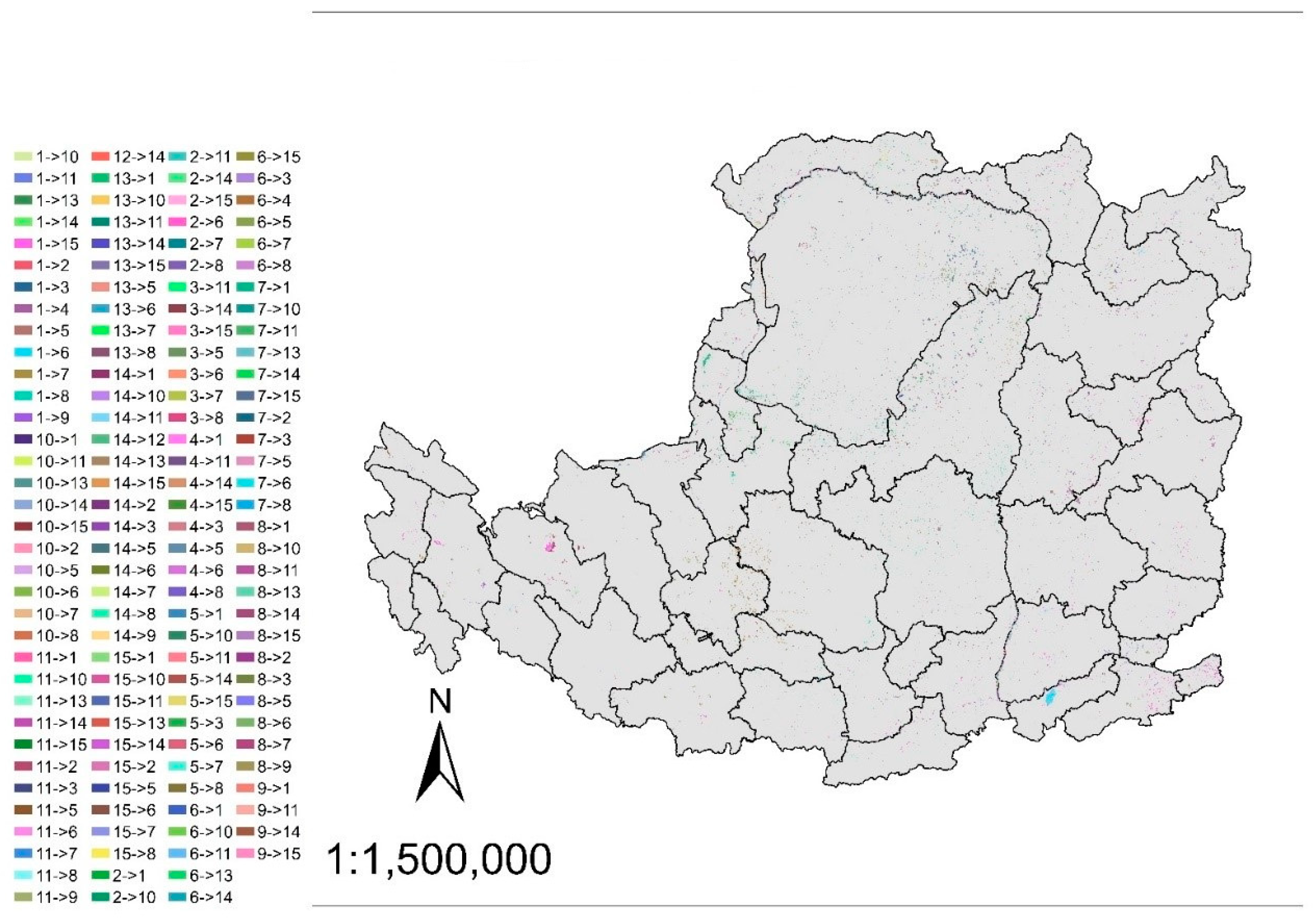
3.1. LULC Conversion between 1990 and 2015
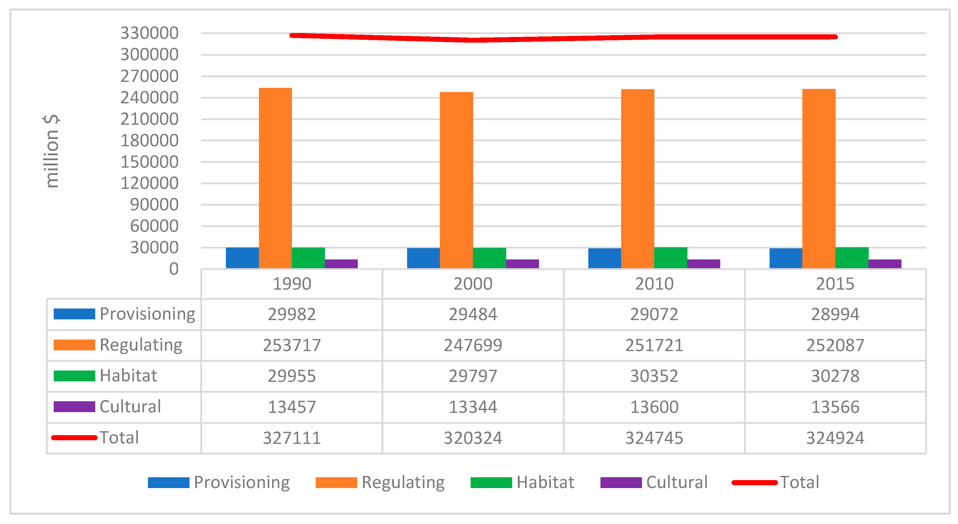
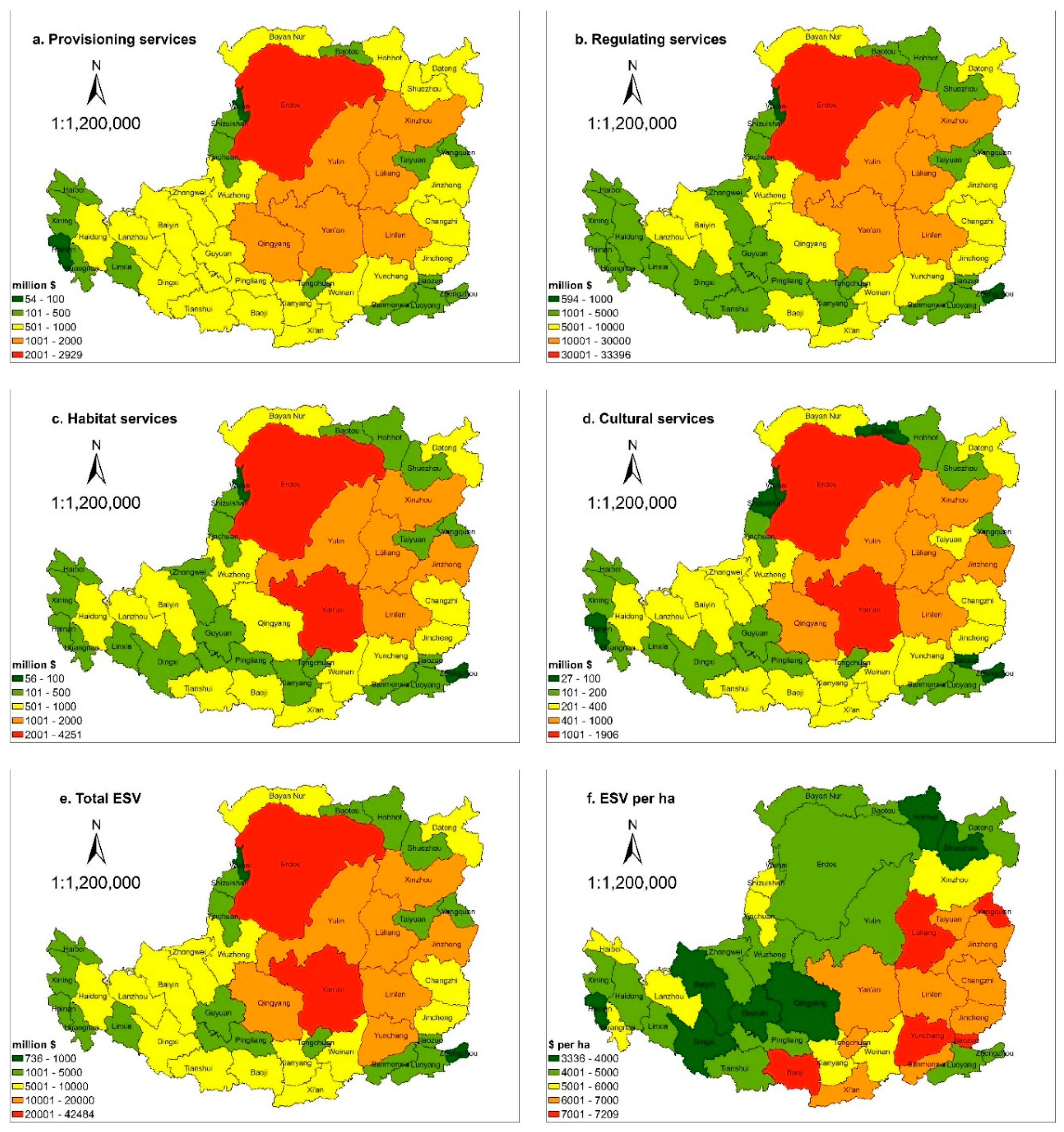
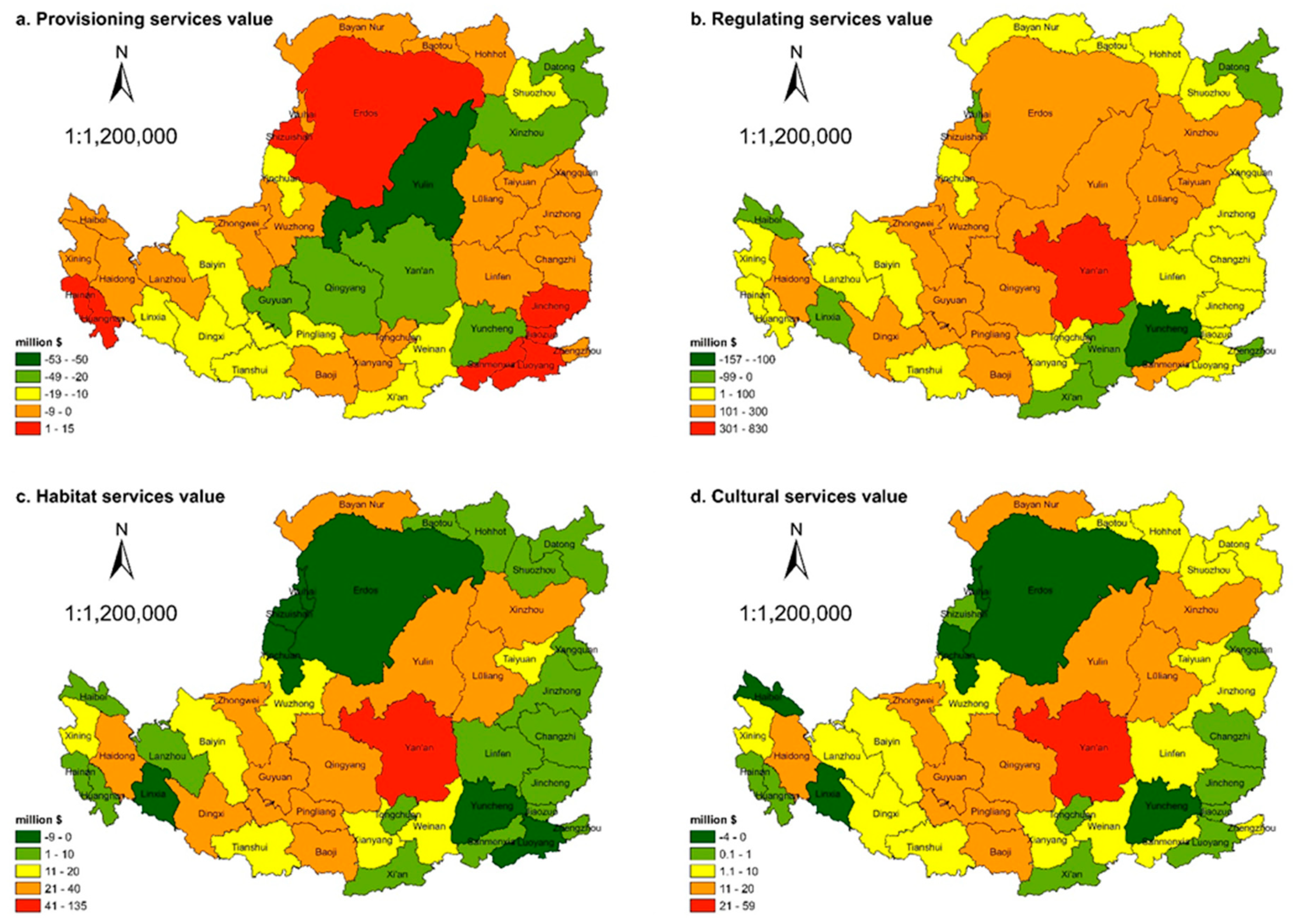
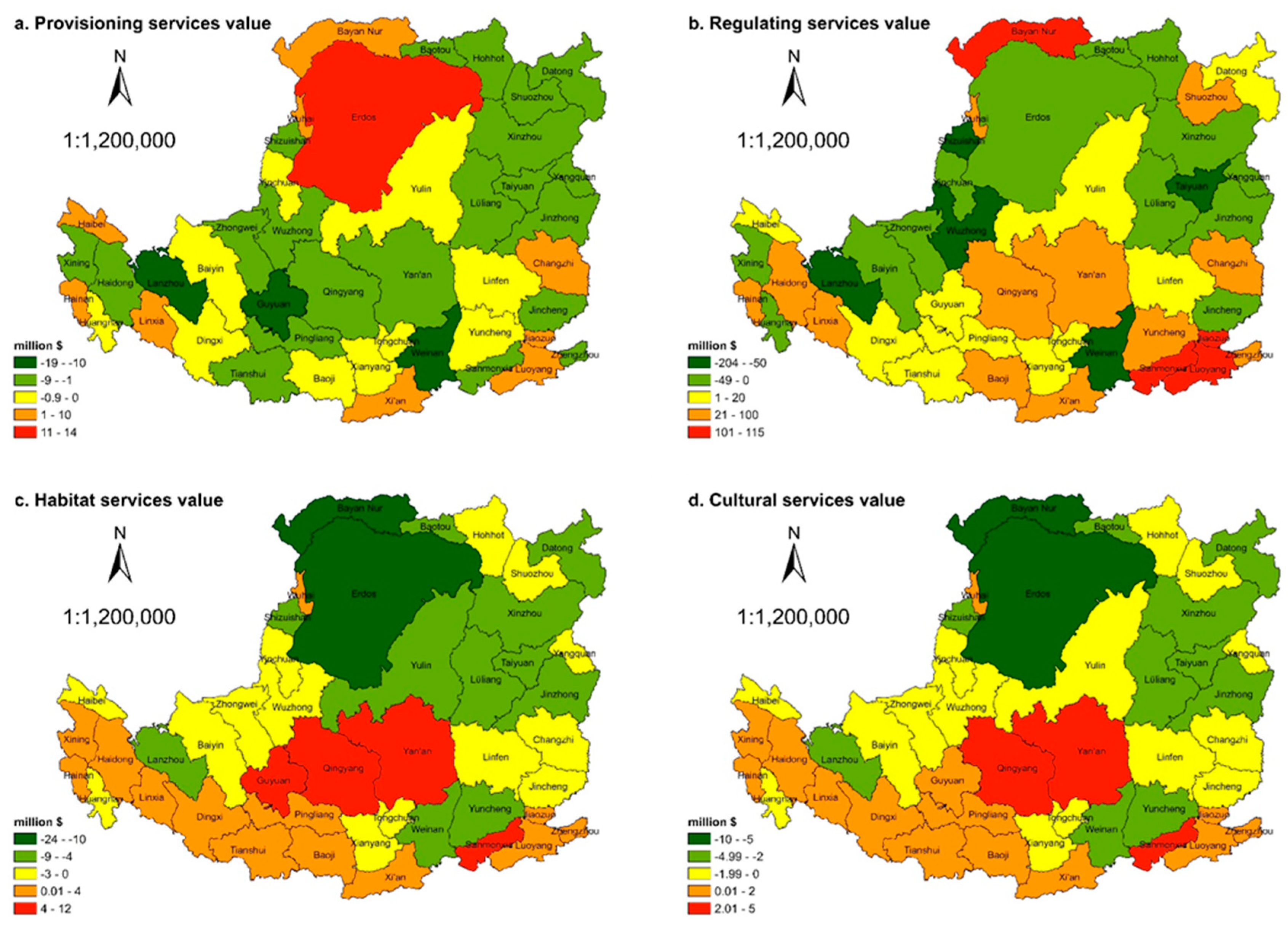
3.2. ESV Changes between 1990 and 2015
3.3. Elasticity Analysis
4. Discussion
4.1. The Implications for Policy-Making
4.2. The Driving Factors for LULC Conversion on the LP
4.3. The Improvement of Accuracy
5. Conclusions
Author Contributions
Funding
Acknowledgments
Conflicts of Interest
Appendix A


| To | Dry Farmland | Paddy Field | Coniferous Forest | Mixed Forest | Broad-Leaved Forest | Bush | Prairie | Shrub Grass | Meadow | Wetland | River and Lake | Glacier and Snow | Desert | Bare Land | Built-Up Area | |
|---|---|---|---|---|---|---|---|---|---|---|---|---|---|---|---|---|
| From | ||||||||||||||||
| Dry farmland | - | 1987 | 148 | 516 | 9546 | 54,646 | 55,740 | 80,831 | 2073 | 1732 | 20,191 | 0 | 103 | 13,628 | 149,663 | |
| Paddy field | 8208 | - | 0 | 2 | 1 | 235 | 208 | 73 | 0 | 112 | 811 | 0 | 0 | 21 | 1772 | |
| Coniferous forest | 121 | 0 | - | 153 | 788 | 1732 | 227 | 661 | 149 | 0 | 16 | 0 | 0 | 30 | 13 | |
| Mixed forest | 315 | 0 | 259 | - | 2410 | 1208 | 36 | 274 | 9 | 1 | 36 | 0 | 0 | 25 | 38 | |
| Broad-leaved forest | 2721 | 0 | 762 | 909 | - | 7666 | 998 | 2233 | 74 | 0 | 79 | 0 | 10 | 101 | 356 | |
| Bush | 23,520 | 30 | 1321 | 707 | 7781 | - | 13,140 | 11,528 | 1682 | 90 | 619 | 0 | 2979 | 839 | 3201 | |
| Prairie | 74,943 | 848 | 192 | 32 | 822 | 10,057 | - | 13,438 | 843 | 1044 | 2576 | 1 | 6141 | 5272 | 10,663 | |
| Shrub grass | 107,384 | 5365 | 646 | 223 | 2562 | 20,085 | 22,741 | - | 118 | 514 | 4003 | 23 | 6697 | 18,583 | 19,445 | |
| Meadow | 1179 | 0 | 62 | 2 | 12 | 1175 | 708 | 112 | - | 7 | 3 | 0 | 0 | 182 | 103 | |
| Wetland | 7630 | 199 | 1 | 0 | 14 | 308 | 952 | 594 | 29 | - | 8020 | 0 | 3 | 1760 | 199 | |
| River and lake | 75,876 | 5346 | 6 | 66 | 423 | 3280 | 8405 | 10,936 | 7 | 10,818 | - | 0 | 729 | 37,079 | 2820 | |
| Glacier and snow | 0 | 0 | 0 | 0 | 0 | 1 | 2 | 0 | 0 | 0 | 0 | - | 0 | 6776 | 0 | |
| Desert | 5387 | 0 | 0 | 0 | 10 | 4900 | 14,641 | 20,722 | 1 | 42 | 22 | 0 | - | 416 | 398 | |
| Bare land | 111,765 | 5748 | 22 | 21 | 166 | 5552 | 9969 | 20,863 | 171 | 1007 | 13,916 | 1438 | 111 | - | 8263 | |
| Built-up area | 7456 | 67 | 15 | 5 | 224 | 504 | 788 | 806 | 10 | 6 | 97 | 0 | 12 | 147 | - | |
| To | Dry Farmland | Paddy Field | Coniferous Forest | Mixed Forest | Broad-Leaved Forest | Bush | Prairie | Shrub Grass | Meadow | Wetland | River and Lake | Glacier and Snow | Desert | Bare Land | Built-Up Area | |
|---|---|---|---|---|---|---|---|---|---|---|---|---|---|---|---|---|
| From | ||||||||||||||||
| Dry farmland | - | 8706 | 577 | 1252 | 27,139 | 232,021 | 595,344 | 320,514 | 16,900 | 6967 | 40,955 | 0 | 306 | 36,357 | 254,592 | |
| Paddy field | 9912 | - | 0 | 0 | 17 | 214 | 102 | 43 | 29 | 1709 | 0 | 0 | 76 | 1192 | ||
| Coniferous forest | 84 | 0 | - | 157 | 2099 | 707 | 35 | 307 | 4 | 0 | 13 | 0 | 0 | 16 | 80 | |
| Mixed forest | 141 | 0 | 147 | - | 925 | 544 | 18 | 237 | 0 | 0 | 5 | 0 | 0 | 5 | 37 | |
| Broad-leaved forest | 2089 | 3 | 2773 | 874 | - | 10,033 | 496 | 1791 | 0 | 0 | 222 | 0 | 0 | 243 | 677 | |
| Bush | 11,926 | 4 | 928 | 664 | 13,485 | - | 6004 | 8944 | 124 | 27 | 725 | 0 | 668 | 1280 | 8654 | |
| Prairie | 58,295 | 692 | 181 | 20 | 728 | 13,773 | - | 8518 | 235 | 1731 | 6308 | 1 | 4097 | 13,008 | 75,909 | |
| Shrub grass | 45,516 | 1790 | 225 | 292 | 2124 | 19,979 | 17,254 | - | 12 | 1081 | 10,787 | 6 | 6484 | 12,744 | 54,031 | |
| Meadow | 60 | 0 | 13 | 1 | 0 | 566 | 165 | 2 | - | 0 | 23 | 2 | 0 | 6 | 319 | |
| Wetland | 3758 | 78 | 0 | 0 | 96 | 627 | 2257 | 764 | 0 | - | 8015 | 0 | 6 | 1669 | 1030 | |
| River and lake | 21,206 | 3324 | 27 | 19 | 155 | 2411 | 5804 | 5545 | 5 | 10,028 | - | 0 | 110 | 18,747 | 4779 | |
| Glacier and snow | 0 | 0 | 0 | 0 | 0 | 0 | 0 | 0 | 0 | 0 | 0 | - | 0 | 0 | 0 | |
| Desert | 2300 | 30 | 192 | 2193 | 12,381 | 15,616 | 0 | 0 | 0 | 127 | 167 | 0 | - | 521 | 4260 | |
| Bare land | 30,622 | 584 | 13 | 18 | 361 | 3921 | 12,391 | 14,113 | 130 | 3567 | 26,562 | 2878 | 580 | - | 24,159 | |
| Built-up area | 10,118 | 636 | 1 | 3 | 68 | 347 | 114 | 470 | 1 | 11 | 233 | 0 | 1 | 86 | - | |
| To | Dry Farmland | Paddy Field | Coniferous Forest | Mixed Forest | Broad-Leaved Forest | Bush | Prairie | Shrub Grass | Meadow | Wetland | River and Lake | Glacier and Snow | Desert | Bare Land | Built-Up Area | |
|---|---|---|---|---|---|---|---|---|---|---|---|---|---|---|---|---|
| From | ||||||||||||||||
| Dry farmland | - | 1466 | 0 | 1 | 833 | 24,214 | 117,626 | 50,456 | 2576 | 1358 | 21,071 | 0 | 58 | 15,245 | 106,479 | |
| Paddy field | 577 | - | 0 | 0 | 0 | 401 | 598 | 35 | 0 | 0 | 2403 | 0 | 0 | 243 | 4878 | |
| Coniferous forest | 0 | 0 | - | 0 | 3 | 16 | 10 | 5 | 0 | 0 | 5 | 0 | 0 | 12 | 476 | |
| Mixed forest | 32 | 0 | 0 | - | 0 | 1 | 0 | 44 | 0 | 0 | 0 | 0 | 0 | 17 | 347 | |
| Broad-leaved forest | 795 | 0 | 2 | 0 | - | 94 | 107 | 198 | 0 | 0 | 111 | 0 | 0 | 443 | 2006 | |
| Bush | 9877 | 0 | 9 | 0 | 2835 | - | 1375 | 745 | 0 | 88 | 949 | 0 | 96 | 3043 | 15,688 | |
| Prairie | 64,399 | 5 | 0 | 0 | 72 | 2868 | - | 2765 | 0 | 157 | 5665 | 0 | 715 | 12,980 | 61,211 | |
| Shrub grass | 33,188 | 0 | 0 | 0 | 100 | 1552 | 3538 | - | 5 | 323 | 5751 | 0 | 1622 | 20,920 | 40,445 | |
| Meadow | 199 | 0 | 0 | 0 | 0 | 0 | 0 | 0 | - | 0 | 265 | 0 | 0 | 1170 | 213 | |
| Wetland | 3183 | 66 | 0 | 0 | 24 | 277 | 1819 | 554 | 0 | - | 13,052 | 0 | 6 | 2248 | 654 | |
| River and lake | 8542 | 2103 | 1 | 0 | 28 | 1120 | 6936 | 5251 | 26 | 4903 | - | 0 | 117 | 17,418 | 624 | |
| Glacier and snow | 0 | 0 | 0 | 0 | 0 | 0 | 0 | 0 | 0 | 0 | 0 | - | 0 | 454 | 0 | |
| Desert | 5372 | 0 | 0 | 0 | 55 | 3780 | 12,277 | 13,866 | 0 | 67 | 98 | 0 | - | 3146 | 5759 | |
| Bare land | 11,939 | 58 | 0 | 0 | 21 | 1879 | 7017 | 6481 | 96 | 1216 | 16,630 | 0 | 2921 | - | 10,478 | |
| Built-up area | 38 | 0 | 0 | 0 | 2 | 39 | 7 | 31 | 0 | 3 | 660 | 0 | 1 | 14 | - | |


References
- Millennium ecosystem assessment. In Ecosystems and Human Well-Being: Synthesis; Island Press: Washington, DC, USA, 2005.
- The Economics of Ecosystems and Biodiversity: Mainstreaming the Economics of Nature: A synthesis of the Approach, Conclusions and Recommendations of TEEB; UNEP: Nairobi, Kenya, 2010.
- Costanza, R.; D’Arge, R.; De Groot, R.; Farber, S.; Grasso, M.; Hannon, B.; Limburg, K.; Naeem, S.; O’Neill, R.V.; Paruelo, J.; et al. The value of the world’s ecosystem services and natural capital. Nature 1997, 387, 253–260. [Google Scholar] [CrossRef]
- De Groot, R.; Brander, L.; Van Der Ploeg, S.; Costanza, R.; Bernard, F.; Braat, L.; Christie, M.; Crossman, N.; Ghermandi, A.; Hein, L.; et al. Global estimates of the value of ecosystems and their services in monetary units. Ecosyst. Serv. 2012, 1, 50–61. [Google Scholar] [CrossRef]
- Bateman, I.J.; Harwood, A.R.; Mace, G.M.; Watson, R.T.; Abson, D.J.; Andrews, B.; Binner, A.; Crowe, A.; Day, B.H.; Dugdale, S.; et al. Bringing ecosystem services into economic decision-making: Land use in the United Kingdom. Science 2013, 341, 45–50. [Google Scholar] [CrossRef] [PubMed]
- Fu, B.; Zhang, L.; Xu, Z.; Zhao, Y.; Wei, Y.; Skinner, D. Ecosystem services in changing land use. J. Soils Sediments 2015, 15, 833–843. [Google Scholar] [CrossRef]
- Costanza, R.; De Groot, R.; Sutton, P.; Van der Ploeg, S.; Anderson, S.J.; Kubiszewski, I.; Farber, S.; Turner, R.K. Changes in the global value of ecosystem services. Glob. Environ. Chang. 2014, 26, 152–158. [Google Scholar] [CrossRef]
- Schägner, J.; Brander, L.; Maes, J.; Hartje, V. Mapping ecosystem services’ values: Current practice and future prospects. Ecosyst. Serv. 2013, 4, 33–46. [Google Scholar] [CrossRef]
- Kindu, M.; Schneider, T.; Teketay, D.; Knoke, T. Changes of ecosystem service values in response to land use/land cover dynamics in Munessa-Shashemene landscape of the Ethiopian highlands. Sci. Total Environ. 2016, 547, 137–147. [Google Scholar] [CrossRef]
- Song, W.; Deng, X. Land-use/land-cover change and ecosystem service provision in China. Sci. Total Environ. 2017, 576, 705–719. [Google Scholar] [CrossRef]
- Arowolo, A.O.; Deng, X.; Olatunji, O.A.; Obayelu, A.E. Assessing changes in the value of ecosystem services in response to land-use/land-cover dynamics in Nigeria. Sci. Total Environ. 2018, 636, 597–609. [Google Scholar] [CrossRef]
- Zhang, F.; Yushanjiang, A.; Jing, Y. Assessing and predicting changes of the ecosystem service values based on land use/cover change in Ebinur Lake Wetland National Nature Reserve, Xinjiang, China. Sci. Total Environ. 2019, 656, 1133–1144. [Google Scholar] [CrossRef]
- Qiu, B.; Li, H.; Zhou, M.; Zhang, L. Vulnerability of ecosystem services provisioning to urbanization: A case of China. Ecol. Indic. 2015, 57, 505–513. [Google Scholar] [CrossRef]
- Liu, W.; Yan, Y.; Wang, D.; Ma, W. Integrate carbon dynamics models for assessing the impact of land use intervention on carbon sequestration ecosystem service. Ecol. Indic. 2018, 91, 268–277. [Google Scholar] [CrossRef]
- Salata, S.; Ronchi, S.; Arcidiacono, A. Mapping air filtering in urban areas. A Land Use Regression model for Ecosystem Services assessment in planning. Ecosyst. Serv. 2017, 28, 341–350. [Google Scholar] [CrossRef]
- Brauman, K.A.; Freyberg, D.L.; Daily, G. Impacts of Land-Use Change on Groundwater Supply: Ecosystem Services Assessment in Kona, Hawaii. J. Water Resour. Plann. Manag. 2015, 141. [Google Scholar] [CrossRef]
- Lavelle, P.; Rodríguez, N.; Arguello, O.; Bernal, J.; Botero, C.; Chaparro, P.; Gómez, Y.; Gutiérrez, A.; Del Pilar Hurtado, M.; Loaiza, S.; et al. Soil ecosystem services and land use in the rapidly changing Orinoco River Basin of Colombia. Agric. Ecosyst. Environ. 2014, 185, 106–117. [Google Scholar] [CrossRef]
- Butler, J.R.A.; Wong, G.Y.; Metcalfe, D.J.; Honzák, M.; Pert, P.L.; Rao, N.; Van Grieken, M.E.; Lawson, T.; Bruce, C.; Kroon, F.J.; et al. An analysis of trade-offs between multiple ecosystem services and stakeholders linked to land use and water quality management in the Great Barrier Reef, Australia. Agric. Ecosyst. Environ. 2013, 180, 176–191. [Google Scholar] [CrossRef]
- Bozzola, M.; Massetti, E.; Mendelsohn, R.; Capitanio, F. A Ricardian analysis of the impact of climate change on Italian agriculture. Eur. Rev. Agric. Econ. 2018, 45, 57–79. [Google Scholar] [CrossRef]
- Chavas, J.-P.; Di Falco, S.; Adinolfi, F.; Capitanio, F. Weather effects and their long-term impact on the distribution of agricultural yields: Evidence from Italy. Eur. Rev. Agric. Econ. 2019, 46, 29–51. [Google Scholar] [CrossRef]
- Capitanio, F.; Gatto, E.; Millemaci, E. CAP payments and spatial diversity in cereal crops: An analysis of Italian farms. Land Use Policy 2016, 54, 574–582. [Google Scholar] [CrossRef]
- Pascucci, S.; de-Magistris, T.; Dries, L.; Adinolfi, F.; Capitanio, F. Participation of Italian farmers in rural development policy. Eur. Rev. Agric. Econ. 2013, 40, 605–631. [Google Scholar] [CrossRef]
- Cumming, G.S.; Buerkert, A.; Hoffmann, E.M.; Schlecht, E.; Von Cramon-Taubadel, S.; Tscharntke, T. Implications of agricultural transitions and urbanization for ecosystem services. Nature 2014, 515, 50–57. [Google Scholar] [CrossRef] [PubMed]
- Cariveau, D.P.; Williams, N.M.; Benjamin, F.E.; Winfree, R. Response diversity to land use occurs but does not consistently stabilize ecosystem services provided by native pollinators. Ecol. Lett. 2013, 16, 903–911. [Google Scholar] [CrossRef] [PubMed]
- Fontana, V.; Radtke, A.; Walde, J.; Tasser, E.; Wilhalm, T.; Zerbe, S.; Tappeiner, U. What plant traits tell us: Consequences of land-use change of a traditional agro-forest system on biodiversity and ecosystem service provision. Agric. Ecosyst. Environ. 2014, 186, 44–53. [Google Scholar] [CrossRef]
- Byrd, K.B.; Flint, L.E.; Alvarez, P.; Casey, C.F.; Sleeter, B.M.; Soulard, C.E.; Flint, A.L.; Sohl, T.L. Integrated climate and land use change scenarios for California rangeland ecosystem services: Wildlife habitat, soil carbon, and water supply. Landsc. Ecol 2015, 30, 729–750. [Google Scholar] [CrossRef]
- Feng, X.; Fu, B.; Lu, N.; Zeng, Y.; Wu, B. How ecological restoration alters ecosystem services: An analysis of carbon sequestration in China’s Loess Plateau. Sci. Rep. 2013, 3, 2846. [Google Scholar] [CrossRef]
- Wu, D.; Zou, C.; Cao, W.; Xiao, T.; Gong, G. Ecosystem services changes between 2000 and 2015 in the Loess Plateau, China: A response to ecological restoration. PLoS ONE 2019, 14, e0209483. [Google Scholar] [CrossRef]
- Jiang, C.; Zhang, H.; Zhang, Z. Spatially explicit assessment of ecosystem services in China’s Loess Plateau: Patterns, interactions, drivers, and implications. Glob. Planet. Chang. 2018, 161, 41–52. [Google Scholar] [CrossRef]
- Wei, H.; Fan, W.; Ding, Z.; Weng, B.; Xing, K.; Wang, X.; Lu, N.; Ulgiati, S.; Dong, X. Ecosystem Services and Ecological Restoration in the Northern Shaanxi Loess Plateau, China, in Relation to Climate Fluctuation and Investments in Natural Capital. Sustainability 2017, 9, 199. [Google Scholar] [CrossRef]
- Luo, Y.; Lü, Y.; Fu, B.; Zhang, Q.; Li, T.; Hu, W.; Comber, A. Half century change of interactions among ecosystem services driven by ecological restoration: Quantification and policy implications at a watershed scale in the Chinese Loess Plateau. Sci. Total Environ. 2019, 651, 2546–2557. [Google Scholar] [CrossRef]
- Hou, Y.; Lü, Y.; Chen, W.; Fu, B. Temporal variation and spatial scale dependency of ecosystem service interactions: A case study on the central Loess Plateau of China. Landsc. Ecol. 2017, 32, 1201–1217. [Google Scholar] [CrossRef]
- Su, C.; Fu, B. Evolution of ecosystem services in the Chinese Loess Plateau under climatic and land use changes. Glob. Planet. Chang. 2013, 101, 119–128. [Google Scholar] [CrossRef]
- Shang, X.; Li, X. Holocene vegetation characteristics of the southern Loess Plateau in the Weihe River valley in China. Rev. Palaeobot. Palynol. 2010, 160, 46–52. [Google Scholar] [CrossRef]
- Wang, L.; Shao, M.; Wang, Q.; Gale, W.L. Historical changes in the environment of the Chinese Loess Plateau. Environ. Sci. Policy 2006, 9, 675–684. [Google Scholar] [CrossRef]
- Cai, Q.G. Soil erosion and management on the Loess Plateau. J. Geogr. Sci. 2001, 11, 53–70. [Google Scholar] [CrossRef]
- Fu, B.; Liu, Y.; Lü, Y.; He, C.; Zeng, Y.; Wu, B. Assessing the soil erosion control service of ecosystems change in the Loess Plateau of China. Ecol. Complex. 2011, 8, 284–293. [Google Scholar] [CrossRef]
- Lü, Y.; Fu, B.; Feng, X.; Zeng, Y.; Liu, Y.; Chang, R.; Sun, G.; Wu, B. A policy-driven large scale ecological restoration: Quantifying ecosystem services changes in the Loess Plateau of China. PLoS ONE 2012, 7, e31782. [Google Scholar] [CrossRef]
- Wu, B.; Qian, J.; Zeng, Y. Land Cover Atlas of the People’s Republic of China (1:1,000,000); SinoMaps Press: Beijing, China, 2017.
- Xie, G.; Zhang, C.; Zhen, L.; Zhang, L. Dynamic changes in the value of China’s ecosystem services. Ecosyst. Serv. 2017, 26, 146–154. [Google Scholar] [CrossRef]
- Plummer, M.L. Assessing benefit transfer for the valuation of ecosystem services. Front. Ecol. Environ. 2009, 7, 38–45. [Google Scholar] [CrossRef]
- Richardson, L.; Loomis, J.; Kroeger, T.; Casey, F. The role of benefit transfer in ecosystem service valuation. Ecol. Econ. 2015, 115, 51–58. [Google Scholar] [CrossRef]
- Xie, G.; Lu, C.; Leng, Y.; Zheng, D.; Li, S. Ecological assets valuation of the Tibetan Plateau. J. Nat. Resour. 2003, 18, 189–196. (In Chinese) [Google Scholar]
- Jiang, W.; Lü, Y.; Liu, Y.; Gao, W. Ecosystem service value of the Qinghai-Tibet Plateau significantly increased during 25 years. Ecosyst. Serv. 2020, 44, 101146. [Google Scholar] [CrossRef]
- Crespo-Cebada, E.; Díaz-Caro, C.; Robina-Ramírez, R.; Sánchez-Hernández, M.I. Is Biodiversity a Relevant Attribute for Assessing Natural Parks? Evidence from Cornalvo Natural Park in Spain. Forests 2020, 11, 410. [Google Scholar] [CrossRef]
- Jenkins, C.N.; Joppa, L. Expansion of the global terrestrial protected area system. Biol. Conserv. 2009, 142, 2166–2174. [Google Scholar] [CrossRef]
- Ren, Y.; Lü, Y.; Fu, B.; Comber, A.; Li, T.; Hu, J. Driving Factors of Land Change in China’s Loess Plateau: Quantification Using Geographically Weighted Regression and Management Implications. Remote Sens. 2020, 12, 453. [Google Scholar] [CrossRef]
- Du, X.; Zhao, X.; Liang, S.; Zhao, J.; Xu, P.; Wu, D. Quantitatively Assessing and Attributing Land Use and Land Cover Changes on China’s Loess Plateau. Remote Sens. 2020, 12, 353. [Google Scholar] [CrossRef]
- Foody, G.M. Valuing map validation: The need for rigorous land cover map accuracy assessment in economic valuations of ecosystem services. Ecol. Econ. 2015, 111, 23–28. [Google Scholar] [CrossRef]
- Song, X.-P. Global Estimates of Ecosystem Service Value and Change: Taking into Account Uncertainties in Satellite-based Land Cover Data. Ecol. Econ. 2018, 143, 227–235. [Google Scholar] [CrossRef]
- Yang, H.; Li, S.; Chen, J.; Zhang, X.; Xu, S. The Standardization and Harmonization of Land Cover Classification Systems towards Harmonized Datasets: A Review. Int. J. Geo-Inf. 2017, 6, 154. [Google Scholar] [CrossRef]
- Song, P.; Kim, G.; Mayer, A.; He, R.; Tian, G. Assessing the Ecosystem Services of Various Types of Urban Green Spaces Based on i-Tree Eco. Sustainability 2020, 12, 1630. [Google Scholar] [CrossRef]
- Xie, Q.; Yue, Y.; Sun, Q.; Chen, S.; Lee, S.; Kim, S.W. Assessment of Ecosystem Service Values of Urban Parks in Improving Air Quality: A Case Study of Wuhan, China. Sustainability 2019, 11, 6519. [Google Scholar] [CrossRef]


| LULC [40] | China Cover [39] |
|---|---|
| Dry farmland | Dry farmland |
| Paddy field | Paddy field |
| Coniferous forest | Evergreen needleleaf forest |
| Deciduous needleleaf forest | |
| Mixed forest | Broadleaf and needleleaf mixed forest |
| Broad-leaved forest | Evergreen broadleaf forest |
| Deciduous broadleaf forest | |
| Bush | Evergreen broadleaf shrubland |
| Deciduous broadleaf shrubland | |
| Evergreen needleleaf shrubland | |
| Sparse forest | |
| Sparse shrubland | |
| Tree orchard | |
| Shrub orchard | |
| Tree garden | |
| Shrub garden | |
| Prairie | Temperate steppe |
| Alpine steppe | |
| Shrub grass | Tussock |
| Sparse grassland | |
| Lawn | |
| Meadow | Temperate meadow |
| Alpine meadow | |
| Wetland | Tree wetland |
| Shrub wetland | |
| Herbaceous wetland | |
| River and lake | Lake |
| Reservoir/pond | |
| River | |
| Canal/channel | |
| Glacier and snow | Permanent ice/snow |
| Desert | Moss/lichen |
| Gobi | |
| Desert | |
| Bare land | Bare rock |
| Bare soil | |
| Salina | |
| Built-up area | Settlement |
| Transportation land | |
| Mining field |
| LULC | Provisioning Services | Regulating Services | Habitat Services | Cultural Services | |||||||
|---|---|---|---|---|---|---|---|---|---|---|---|
| Food | Materials | Water | Air Quality Regulation | Climate Regulation | Waste Treatment | Water Flow Regulation | Erosion Prevention | Soil Fertility Maintenance | |||
| Dry farmland | 427.72 | 201.28 | 10.06 | 337.14 | 181.15 | 50.32 | 135.86 | 518.3 | 60.38 | 65.42 | 30.19 |
| Paddy field | 684.35 | 45.29 | -1323.42 | 558.55 | 286.82 | 85.54 | 1368.7 | 5.03 | 95.61 | 105.67 | 45.29 |
| Coniferous forest | 110.7 | 261.66 | 135.86 | 855.44 | 2551.22 | 749.77 | 1680.69 | 1036.59 | 80.51 | 946.02 | 412.62 |
| Mixed forest | 155.99 | 357.27 | 186.18 | 1182.52 | 3537.5 | 1001.37 | 1766.23 | 1439.15 | 110.7 | 1308.32 | 573.65 |
| Broad-leaved forest | 145.93 | 332.11 | 171.09 | 1091.94 | 3270.8 | 971.18 | 2385.17 | 1333.48 | 100.64 | 1212.71 | 533.39 |
| Bush | 95.61 | 216.38 | 110.7 | 709.51 | 2128.54 | 644.1 | 1685.72 | 865.5 | 65.42 | 790.02 | 347.21 |
| Prairie | 50.32 | 70.45 | 40.26 | 256.63 | 674.29 | 221.41 | 493.14 | 311.98 | 25.16 | 281.79 | 125.8 |
| Shrub grass | 191.22 | 281.79 | 155.99 | 991.3 | 2621.67 | 865.5 | 1922.22 | 1207.68 | 90.58 | 1096.98 | 483.07 |
| Meadow | 110.7 | 166.06 | 90.58 | 573.65 | 1519.66 | 503.2 | 1112.07 | 699.45 | 55.35 | 639.06 | 281.79 |
| Wetland | 256.63 | 251.6 | 1303.29 | 956.08 | 1811.52 | 1811.52 | 12,192.54 | 1162.39 | 90.58 | 3960.18 | 2380.14 |
| River and lake | 402.56 | 115.74 | 4171.53 | 387.46 | 1152.33 | 2792.76 | 51,447.17 | 467.98 | 35.22 | 1283.16 | 951.05 |
| Glacier and snow | 0 | 0 | 1086.91 | 90.58 | 271.73 | 80.51 | 3587.82 | 0 | 0 | 5.03 | 45.29 |
| Desert | 5.03 | 15.1 | 10.06 | 55.35 | 50.32 | 155.99 | 105.67 | 65.42 | 5.03 | 60.38 | 25.16 |
| Bare land | 0 | 0 | 0 | 10.06 | 0 | 50.32 | 15.1 | 10.06 | 0 | 10.06 | 5.03 |
| Built-up area | 0 | 0 | 0 | 0 | 0 | 0 | 0 | 0 | 0 | 0 | 0 |
| Year | 1990 | 2000 | 2010 | 2015 | ||||
|---|---|---|---|---|---|---|---|---|
| LULC | Area (ha) | Percent | Area (ha) | Percent | Area (ha) | Percent | Area (ha) | Percent |
| Dry farmland | 19,472,293 | 31.25% | 19,506,873 | 31.30% | 18,151,785 | 29.13% | 17,947,533 | 28.80% |
| Paddy field | 174,004 | 0.28% | 182,162 | 0.29% | 184,742 | 0.30% | 179,297 | 0.29% |
| Coniferous forest | 1,047,766 | 1.68% | 1,047,277 | 1.68% | 1,048,730 | 1.68% | 1,048,223 | 1.68% |
| Mixed forest | 375,272 | 0.60% | 373,266 | 0.60% | 374,515 | 0.60% | 374,076 | 0.60% |
| Broad-leaved forest | 3,461,729 | 5.56% | 3,470,623 | 5.57% | 3,498,933 | 5.62% | 3,499,165 | 5.62% |
| Bush | 8,460,955 | 13.58% | 8,505,503 | 13.65% | 8,741,112 | 14.03% | 8,742,781 | 14.03% |
| Prairie | 12,116,088 | 19.44% | 12,117,713 | 19.45% | 12,589,808 | 20.20% | 12,590,323 | 20.20% |
| Shrub grass | 10,312,821 | 16.55% | 10,267,643 | 16.48% | 10,473,953 | 16.81% | 10,446,975 | 16.77% |
| Meadow | 777,767 | 1.25% | 779,398 | 1.25% | 795,663 | 1.28% | 796,513 | 1.28% |
| Wetland | 98,295 | 0.16% | 93,982 | 0.15% | 99,295 | 0.16% | 85,520 | 0.14% |
| River and lake | 439,548 | 0.71% | 333,719 | 0.54% | 357,665 | 0.57% | 377,282 | 0.61% |
| Glacier and snow | 10,679 | 0.02% | 5358 | 0.01% | 8248 | 0.01% | 7793 | 0.01% |
| Desert | 1,601,789 | 2.57% | 1,572,011 | 2.52% | 1,546,439 | 2.48% | 1,507,441 | 2.42% |
| Bare land | 2,363,022 | 3.79% | 2,268,582 | 3.64% | 2,233,455 | 3.58% | 2,252,058 | 3.61% |
| Built-up area | 1,602,038 | 2.57% | 1,789,957 | 2.87% | 2,209,725 | 3.55% | 2,459,089 | 3.95% |
| Total | 62,314,068 | 100.00% | 62,314,068 | 100.00% | 62,314,068 | 100.00% | 62,314,068 | 100.00% |
| Period | 1990–2000 | 2000–2010 | 2010–2015 | |
|---|---|---|---|---|
| LULC | ||||
| Dry farmland | 0.38 | 0.39 | 0.39 | |
| Paddy field | 0.37 | 0.38 | 0.38 | |
| Coniferous forest | 1.68 | 1.72 | 1.69 | |
| Mixed forest | 2.21 | 2.26 | 2.23 | |
| Broad-leaved forest | 2.2 | 2.25 | 2.22 | |
| Bush | 1.46 | 1.49 | 1.47 | |
| Prairie | 0.49 | 0.5 | 0.49 | |
| Shrub grass | 1.89 | 1.93 | 1.9 | |
| Meadow | 1.1 | 1.12 | 1.1 | |
| Wetland | 4.99 | 5.09 | 5.02 | |
| River and lake | 12.04 | 12.3 | 12.13 | |
| Glacier and snow | 0.98 | 1.01 | 0.99 | |
| Desert | 0.11 | 0.11 | 0.11 | |
| Bare land | 0.02 | 0.02 | 0.02 | |
| Period | Total Area (ha) | Converted Area (ha) | Percent | ESV Start (millions of $) | ESV Change (millions of $) | Percent |
|---|---|---|---|---|---|---|
| 1990–2000 | 62,314,068 | 1,250,860 | 2.01% | 327,111 | -6787 | 2.07% |
| 2000–2010 | 62,314,068 | 2,250,331 | 3.61% | 320,324 | 4421 | 1.38% |
| 2010–2015 | 62,314,068 | 823,434 | 1.32% | 324,745 | 179 | 0.06% |
| LULC Change | Area (ha) | ESV Change (millions of $) |
|---|---|---|
| Bare land–River/lake | 1040.15 | 4513.26 |
| Shrub grass–River/lake | 419.94 | 22.38 |
| Dry farmland–River/lake | 25.69 | 1.57 |
| Dry farmland–Shrub grass | 0.09 | 0.001 |
| Dry farmland–Built-up area | 597.24 | −1.21 |
| Total | 2083.12 | 4536.01 |
| LULC Change | Area (ha) | ESV Change (millions of $) |
|---|---|---|
| River/lake–Bare land | 989.76 | −62.46 |
| River/lake–Paddy field | 519.45 | −31.82 |
| River/lake–Prairie | 340.01 | −20.62 |
| River/lake–Shrub grass | 288.15 | −15.36 |
| Shrub grass–Built-up area | 987.35 | −9.78 |
| River/lake–Built-up area | 70.28 | −4.44 |
| Wetland–Prairie | 67.54 | −1.60 |
| Bush–Built-up area | 169.24 | −1.30 |
| Prairie–Built-up area | 497.03 | −1.27 |
| Dry farmland–Built-up area | 570.24 | −1.15 |
| Wetland–Built-up area | 41.67 | −1.09 |
| Wetland–Paddy field | 27.30 | −0.66 |
| River/lake–Bush | 9.03 | −0.50 |
| Wetland–Bare land | 17.25 | −0.45 |
| Paddy field–Bare land | 183.97 | −0.34 |
| Coniferous forest–Built-up area | 37.03 | −0.33 |
| Wetland–Shrub grass | 15.69 | −0.26 |
| Paddy field–Built-up area | 111.84 | −0.22 |
| Shrub grass–Desert | 15.74 | −0.15 |
| Dry farmland–Bare land | 43.29 | −0.08 |
| Bush–Prairie | 16.15 | −0.08 |
| Bare land–Built-up area | 569.28 | −0.06 |
| Desert–Built-up area | 99.97 | −0.06 |
| Wetland–Dry farmland | 1.76 | −0.04 |
| Bush–Bare land | 3.01 | −0.02 |
| Dry farmland–Desert | 3.06 | −0.0045 |
| Desert–Bare land | 1.45 | −0.0007 |
| Prairie–Desert | 0.22 | −0.0004 |
| Dry farmland–Bush | 0.18 | 0.0010 |
| Paddy field–Bush | 1.28 | 0.01 |
| Dry farmland–Prairie | 14.06 | 0.01 |
| Paddy field–Dry farmland | 159.00 | 0.01 |
| Prairie–Shrub grass | 1.68 | 0.01 |
| Bush–Shrub grass | 6.44 | 0.01 |
| Bare land–Prairie | 8.01 | 0.02 |
| Paddy field–Shrub grass | 8.05 | 0.06 |
| Bare land–Shrub grass | 31.73 | 0.31 |
| Paddy field–Prairie | 528.14 | 0.31 |
| Dry farmland–Shrub grass | 71.40 | 0.56 |
| Dry farmland–River/lake | 162.90 | 9.97 |
| Wetland–River/lake | 338.12 | 12.52 |
| Total | 7027.74 | −130.32 |
© 2020 by the authors. Licensee MDPI, Basel, Switzerland. This article is an open access article distributed under the terms and conditions of the Creative Commons Attribution (CC BY) license (http://creativecommons.org/licenses/by/4.0/).
Share and Cite
Jiang, W.; Fu, B.; Lü, Y. Assessing Impacts of Land Use/Land Cover Conversion on Changes in Ecosystem Services Value on the Loess Plateau, China. Sustainability 2020, 12, 7128. https://doi.org/10.3390/su12177128
Jiang W, Fu B, Lü Y. Assessing Impacts of Land Use/Land Cover Conversion on Changes in Ecosystem Services Value on the Loess Plateau, China. Sustainability. 2020; 12(17):7128. https://doi.org/10.3390/su12177128
Chicago/Turabian StyleJiang, Wei, Bojie Fu, and Yihe Lü. 2020. "Assessing Impacts of Land Use/Land Cover Conversion on Changes in Ecosystem Services Value on the Loess Plateau, China" Sustainability 12, no. 17: 7128. https://doi.org/10.3390/su12177128
APA StyleJiang, W., Fu, B., & Lü, Y. (2020). Assessing Impacts of Land Use/Land Cover Conversion on Changes in Ecosystem Services Value on the Loess Plateau, China. Sustainability, 12(17), 7128. https://doi.org/10.3390/su12177128