Self-Learning Algorithm to Predict Indoor Temperature and Cooling Demand from Smart WiFi Thermostat in a Residential Building

Abstract

Smart WiFi thermostats have moved well beyond the function they were originally designed for; namely, controlling heating and cooling comfort in buildings. They are now also learning from occupant behaviors and permit occupants to control their comfort remotely. This research seeks to go beyond this state of the art by utilizing smart WiFi thermostat data in residences to develop dynamic predictive models for room temperature and cooling/heating demand. These models can then be used to estimate the energy savings from new thermostat temperature schedules and estimate peak load reduction achievable from maintaining a residence in a minimum thermal comfort condition. Back Propagation Neural Network (BPNN), Long-Short Term Memory (LSTM), and Encoder-Decoder LSTM dynamic models are explored. Results demonstrate that LSTM outperforms BPNN and Encoder-Decoder LSTM approach, yielding and a MAE error of 0.5 °C, equal to the resolution error of the measured temperature. Additionally, the models developed are shown to be highly accurate in predicting savings from aggressive thermostat set point schedules, yielding deep reduction of up to 14.3% for heating and cooling, as well as significant energy reduction from curtailed thermal comfort in response to a high demand event.

1. Introduction

According to a recent U.S. Energy Information Administration (EIA) report, about 10% of national energy was consumed in the residential sector in 2018 [1]. Concerted efforts to increase energy efficiency in residential buildings have led to substantial reductions in energy use [2]. Yet, while new buildings offer deep savings opportunities from state-of-the-art energy efficient technologies, existing buildings often require comprehensive, extremely costly deep retrofits to achieve comparable savings.

Thermal comfort in buildings has been managed for many years by thermostats. At a most basic level, a thermostat allows a resident to set a desired indoor temperature, a means to sense actual temperature within the thermostat housing, and a means to signal the heating and/or cooling devices to turn on or off in order to affect control of the heating, ventilating, and air conditioning (HVAC) system in order to equilibrate the room temperature to the set point temperature. Thermostats use solid-state sensors such as thermistors or thermal diodes to measure temperature; they also often include humidity sensors for measuring humidity and microprocessor-based circuitry to control the HVAC system and operate based upon user-defined set point schedules. Smart WiFi thermostats communicate set point schedules, measured temperature and humidity, and heating/cooling status to the cloud, where additional processing is possible, while also communicating with the cloud and enabling archival of the thermostat data for each residence.

Since the energy consumption characteristics of residential buildings depend most significantly on the energy characteristics of the residence and behavioral factors, along with the dynamic weather conditions, the residential thermal comfort is always dynamic in nature. This research is premised on a certainty that a predictive data-based model of the indoor temperature measured by the thermostat can play a critical role in executing an effective behavioral energy savings management strategy.

2. Background

Data-driven techniques are frequently used for commercial and residential buildings to elucidate opportunities for energy savings and/or improve occupant comfort. Much of the prior research has focused on testing different data driven approaches to time dependent phenomenon [3,4]. Thomas et al. [3] evaluated the performance of indoor temperature predictive models for two buildings based on linear regression and artificial neural network. The results show the neural network model can achieve better results than linear regression model for indoor temperature prediction. Fan et al. [4] investigated one of the most promising data-drive techniques in predicting 24-h ahead building cooling load. Their results show that deep neural network can enhance the performance of building cooling load prediction compared with other machine learning techniques such as multiple linear regression, random forest, gradient boosting trees, support vector regression, etc. Moreover, Xu et al. [5] recently pointed out that a Long-Short Term Memory (LSTM) model can improve indoor temperature prediction accuracy, and one-time step ahead time-series prediction is more accurate than multi-time step ahead prediction.

One of the most important machine-learning enabled data applications for buildings is the forecasting of heating and cooling demand. A key aspect of this is the prediction of indoor temperature, either in single zones or multiple zones. Such predictions are highly dependent on the features selected as predictors, and upon the measurement frequency of the time-varying predictors. Ruano et al. [6] employed building geometry features, construction materials, and other conditions to predict a building internal temperature using neural networks models. Attoue et al. [7] utilized five-minute interval data from a smart monitoring system that included indoor and outdoor temperature and humidity and solar radiation to predict indoor temperature using an artificial neural network approach. Yu et al. [8] used 5 min interval smart thermostat data and weather forecast data to predict indoor temperature using generalized regression neural network and artificial neural network modeling approaches. Their results showed that adding previous indoor temperature values as predictors can significantly improve the target estimation. All of these efforts, because of the high frequency of collection, required substantial computational time and data storage capacity. Recently Lou et al. [9] developed models from smart WiFi ‘delta’ thermostat data, where data are only collected when there is a change in any of the collected thermostat data fields in order to reduce data storage and computational requirements. Changes in any of these measured features (heating status, cooling status, and fan status, fan control status (on/auto), cool/heat status (cool, heat, off), heating and cooling temperature set-points, thermostat temperature, and humidity ratio) all precipitate collection of all data features for one interval. Lou et al. used these data to develop thermostat-based models using nonlinear autoregressive network with exogenous inputs (NARX) neural network to improve the calculation of the mean radiant temperature (MRT) [9].

This research, like that of Lu et al., also utilizes ‘delta’ smart WiFi thermostat data from individual residences to develop dynamic models to predict one-time step ahead indoor temperature and cooling/heating demand but considers other deep learning algorithms proven more effective for modeling time dependent data. Also, this research uniquely employs the developed models to estimate potential energy savings from more energy effective thermostat setpoint schedules; and to improve the ability to respond to utility peak demand events.

3. Methodology

3.1. Data Collection

Smart WiFi thermostat data were continuously collected from the homes located in the Midwest of the US. The housing set analyzed includes a diversity of houses, with construction years ranging from the early 1900s to present. Included in this set of residences are some new homes built to U.S. Energy Star specifications and older homes that have received variable attention relative to insulation and energy equipment upgrades. Thus, the energy characteristics associated with the homes have significant variation [10].

In this research, the measured data in one residence were collected from 1 June–16 July 2018. This dataset contains 31,670 observations. During this time period, the outdoor temperature ranged from relatively low values where cooling was not required to maximal summer season values. Additionally, historical and real-time weather data aligned with the thermostat data were accessed via the postgres server in Amazon Web Services (AWS). These data include outdoor temperature and outdoor humidity and other weather factors, if needed.

3.2. Data Pre-Processing

The acquired features require preprocessing before model construction and validation [11]. The first pre-processing step aims to establish a uniform period between ‘delta’ thermostat observations, as the models to be developed generally require uniformly sampled data. Two-minute uniformly spaced data observations are created from the two collected data points enveloping the uniform interval using linear interpolation method. ‘Delta’ thermostat data reduce thermostat data storage capacity on average by 95% relative to storage requirements in comparison to two-minute fixed interval thermostat data. Second, the smart WiFi thermostat data were synchronized according to the date/time stamp with outdoor weather data. A nearest neighbor interpolation [12] is used to do this.

Sample smart WiFi thermostat data merged with outdoor weather data are shown in

Table 1. Sample merged WiFi and weather data.

Date	Time	Cooling Set Point (F)	Cooling Status	Indoor Temp.(°F)	Indoor Humidity (%)	Fan Status	Outdoor Temp.(°F)
1 June 2018	14:43	75	100	75.5	58	100	73
…	…	…	…	…	…	…	…
2 June 2018	17:00	80	0	77	57	0	79.3
…	…	…	…	…	…	…	…
3 June 2018	15:00	80	0	77	57	0	74.5
…	…	…	…	…	…	…

below. The cooling status and fan status features are indicated as 0 when the cooling system is off, and 100 if the cooling/heating system is on. Note: If the cooling/heating system is staged and/or the fan unit is variable speed, numbers between 0 and 100 are possible. Third, a correlation matrix (Pearson’s correlation coefficient) and variable importance estimations are utilized to remove redundant features [13] and estimate the importance of features [14]. Last, a Min-Max normalization method was used to scale all data from 0 to 1.

3.3. Evaluating Model Effectiveness and Validation

The entire dataset is divided into training, validation, and testing sets with proportions for these respectively equal to 70%, 15%, and 15%. Training and validation sets are used to respectively train the model and tune model hyperparameters. The testing set as a new dataset is used to evaluate the trained model. The model performance is evaluated using mean absolute error (MAE) and mean absolute percentage error (MAPE). MAE and MAPE can be respectively expressed as below:

$$MAE=\frac{{{\displaystyle \sum }}_i^n\left|y_i-\widehat{y_i}\right|}{n}$$

(1)

$$MAPE=\frac{{{\displaystyle \sum }}_{i=1}^n\frac{\left|y_i-\widehat{y_i}\right|}{y_i}}{n}\times 100$$

(2)

Above $\widehat{y_i}$ is predicted value and $y_i$ is measured or actual value.

3.4. Models Considered

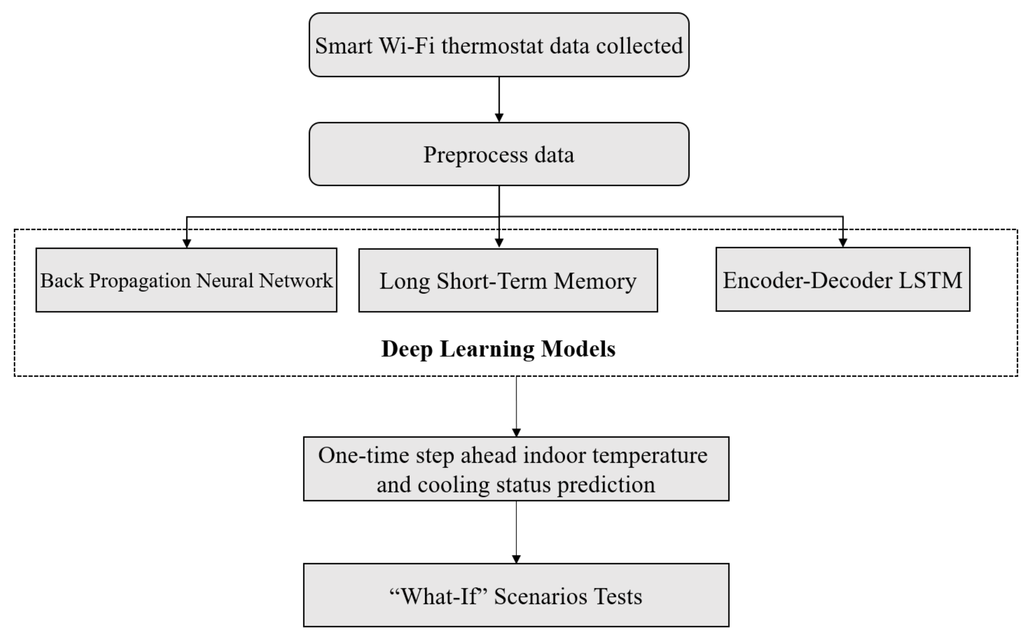
In the background section, neural networks were described as being the best for forecasting time series. In this research, three deep learning neural network algorithms are considered for developing dynamic models to predict one timestep ahead indoor temperature and cooling status; namely Back Propagation Neural Network, Long Short-Term Memory, and Encoder-Decoder LSTM (Long Short-Term Memory). Note that the same approach could be used to predict the heating demand status. All the data analysis and modeling are implemented in R software using the “Keras” package [15]. Figure 1 illustrates the general research outline. The following subsections present an overview of these model approaches, as well as a description of the “What-if’” approach employed to apply the developed models to new set point control scenarios.

3.4.1. Back Propagation Neural Network (BPNN)

Back Propagation Neural Network is one of the most common and effective algorithms used to train artificial neural networks. This method calculates the gradient of the loss function for all weights in the network. Then, the gradient is fed back to the optimization method (such as gradient descent method) to update the weights to minimize the loss function.

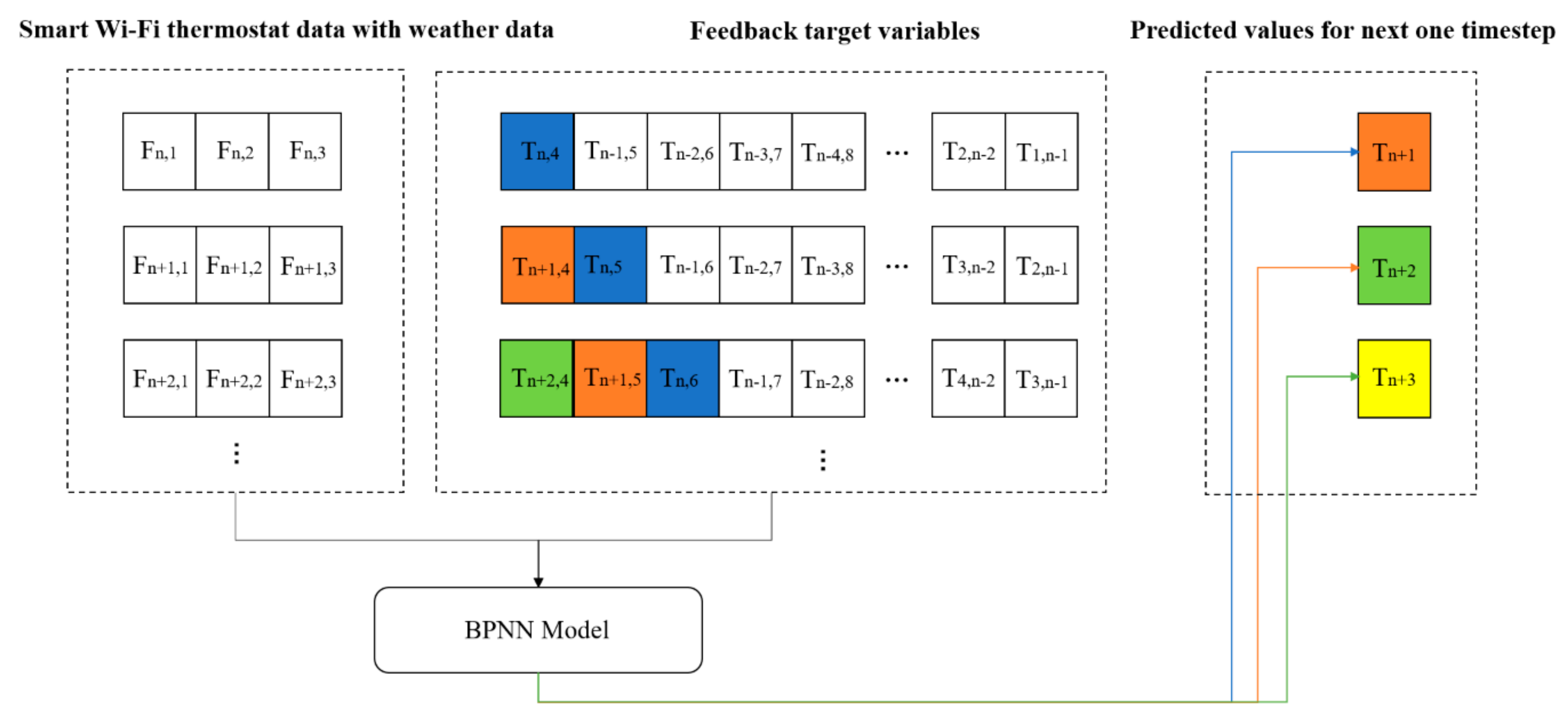
In this research, BPNN is used to develop indoor temperature and cooling status models, using different hyperparameters, e.g., different numbers of layers, numbers of neurons in each layer, dropout ratio, learning rate, and activation function. Here, feedback features are considered as inputs, retaining prior predictions of the target variables as new inputs.

Figure 2 shows the BPNN prediction process for one-time step ahead predictions. In the figure, n is the number of feedback target variables. A value of n = 30 for 2 min uniformly spaced data is associated with a total feedback interval for each observation of 1 h. In this figure, “F” refers to input features or predictors and “T” represents the target variable. Thus, for example, “Fn,1” represents the nth row and first column. In this process, the input features are combined with the smart WiFi thermostat data and feedback target variables. These inputs, as vectors, are fed to a deep learning neural network model to predict the next step. Then, this predicted value is combined with new smart WiFi thermostat data as feedback target variables to form a new input.

3.4.2. Long Short-Term Memory

Long Short-Term Memory (LSTM) is one type of recurrent neural network (RNN), developed by Hochreiter and Schmidhuber in 1997 [16]. Standard RNNs have feedback loops in the recurrent layer that help them memorize the information over time. Retaining every prior predicted target value over a long period of time not only requires substantial computational time in developing a model, but many prior values may not be important for predicting the future value. In fact, these unimportant factors can diminish the quality of the model developed. This leads to what is referred to as a vanishing gradient descent problem. The sensitivity in updating neurons is too small to develop accurate forecasting models [17]. In contrast, LSTM includes memory cells that can store information for long periods of time, and which also ‘forget’ prior values that do not have significance in helping to predict the current target value.

LSTM has three unique gates including a forget gate, an input gate, and an output gate that are able to determine what new input will be stored in the cell state and which data will be deleted (forget gate) [15]. The equations for $f_t$ (forget gate (3)), $i_t$ (input gate (4)), $o_t$ (output gate (5)) are listed below:

$$f_t=\sigma \left(W_f{x}_t+U_f{h}_{t-1}+b_f\right)$$

(3)

$$i_t=\sigma \left(W_i{x}_i+U_i{h}_{t-1}+b_i\right)$$

(4)

$$o_t=\sigma \left(W_o{x}_t+U_o{h}_{t-1}+b_o\right)$$

(5)

$$c_t=f_t\odot c_{t-1}+i_t\odot \tan \mathrm{h}\left(W_c{x}_t+U_c{h}_{t-1}+b_c\right)$$

(6)

$$h_t=o_t\odot tanh\left(c_t\right)$$

(7)

The cell state is updated in a two-part process. The first part (3) consists of the forget gate, and previous cell state: These determine how much the information in the cell state from the previous time step should be kept. The second part (4) is between the input gate and the current cell state. It controls how much of the current information should be allowed into cell state. After updating the current cell state, the current hidden output is computed from the output gate and updated cell state.

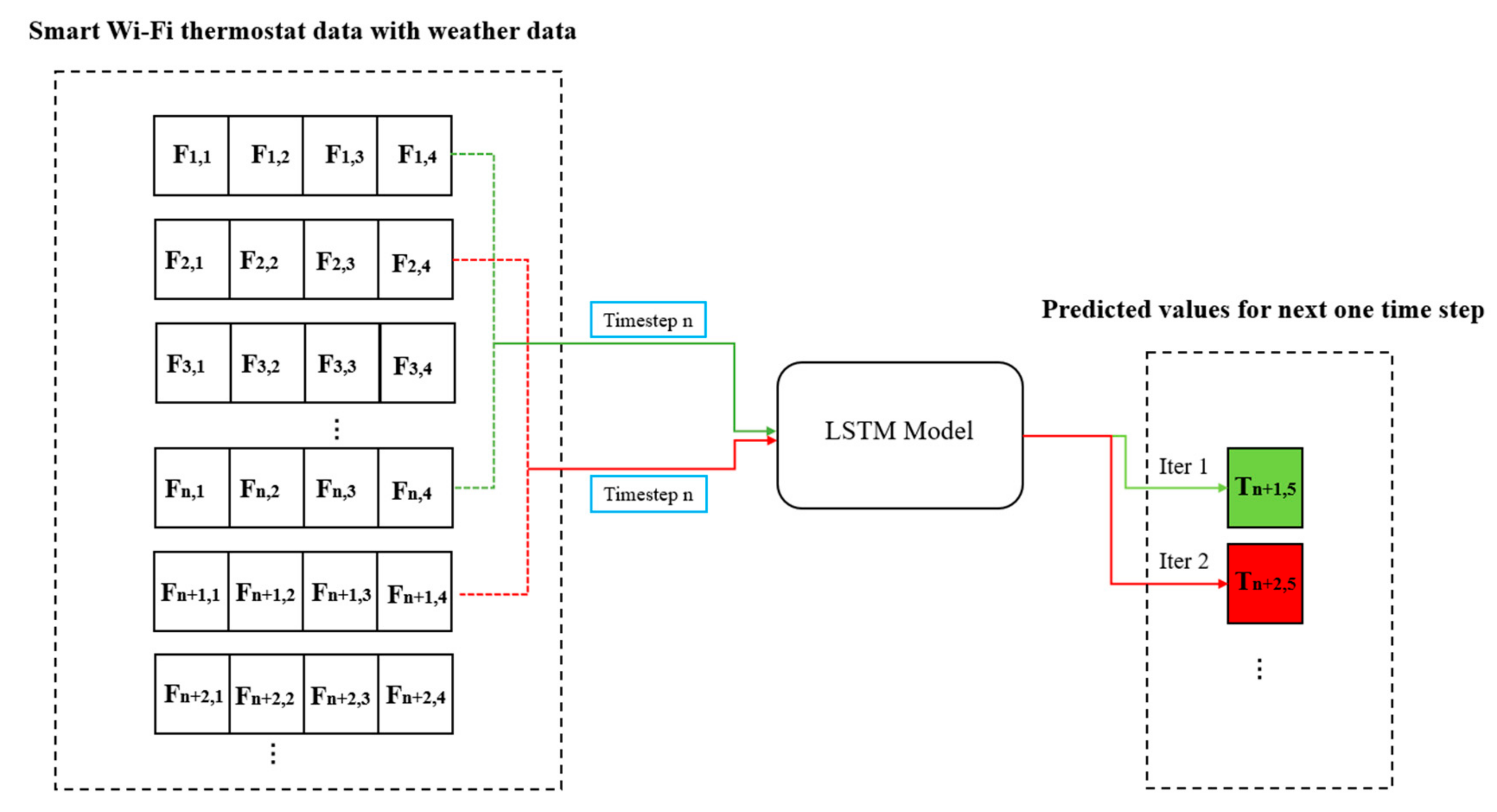
In this research, Long Short-Term Memory is utilized to develop inside residence temperature and cooling demand models to predict the next one-time step target value. The LSTM iterative process for one-time step ahead target prediction is shown in Figure 3. “n” represents the number of prior timesteps considered in the calculation of the next target value.

In the LSTM prediction process, a number of timestep input features are applied to the network model to predict the target at the next step. Compared with the BPNN prediction process, LSTM does not need to generate feedback target variables at each iteration, which accelerates the computational speed.

3.4.3. Encoder-Decoder Long Short-Term Memory Networks (E-D LSTM)

The encoder-decoder recurrent neural network models were widely used for sequence to sequence prediction problems. This algorithm was pioneered in 2014 [18] and has been adopted as the core technology in Google’s translation service [19]. The encoder-decoder recurrent neural network was developed for text translation [20], speech recognition [21], and natural language generation [22]. Until now, only one published paper mentions using encoder-decoder LSTM in weather forecasting problems [23].

The Encoder-Decoder RNN network learns to encode a variable-length sequence into a fixed-length vector representation and to decode a given fixed-length vector representation back into a variable-length sequence. In the E-D RNN encoder part, inputs are read at each timestep and added to the hidden state values from previous timesteps. At the end of the input sequence, it outputs a summary hidden state “c” according to Equation (8) that is meant to encode an entire input sequence.

$$h_t=f\left(h_{t-1},x_t\right)$$

(8)

The E-D RNN decoder part is trained to generate the output sequence by predicting the next symbol Y_T given the hidden state. Both YT and ht are also conditioned on Y_{t−1} and on the summary hidden state c of the input sequence. Hence, the hidden state of the decoder at time t is computed by Equation (9):

$$h_t=f\left(h_{t-1},y_{t-1},c\right)$$

(9)

Then, the conditional distribution of each predicted output is calculated as:

$$P(y_t|y_{t-1},y_{t-2},\dots ,y_1,c)=g\left(h_t,y_{t-1},c\right)$$

(10)

Here, $f$ and $g$ are activation functions that produce valid probabilities.

E-D LSTM is also one type of E-D RNN and it is able to store information for long periods of time. In the E-D LSTM prediction process, feedback variables do not need to be added to the input features to predict the target at the next timestep. Instead, it has the ability to automatically feed the previous target value as an input to predict the next step in the LSTM decoder part.

Figure 4 shows the E-D LSTM prediction process. In this figure, t is the number of timesteps and ${\chi }_t$ represents $1*4$ vector “states” which combine the hidden state and cell state associated with an input sequence. Also, the input sequence is reversed to improve the model performance as indicated from Google team [19].

3.5. “What-If” Scenarios

What-if analysis is a data intensive simulation with the goal to inspect the behavior of a complex system under some given hypotheses called scenarios. In particular, what-if analysis measures how changes in a set of independent or control variables impact a set of dependent variables with reference to a given simulation model [24]. A what-if analysis first requires the establishment of a model. With a model developed, new independent or control variable values can be interrogated provided that their values fall within the range of values present in the training dataset.

The ultimate goal of what-if thermostat scheduling scenarios to be implemented here is to estimate savings from energy saving thermostat set point schedules or to estimate the effect of responding to high demand events while maintaining desired comfort within acceptable bounds.

The effect of different set point schedules ideally linked to zonal occupancy schedules and desired comfort can be evaluated.

Table 2. Three different cooling set point schedules for one day.

Cooling Set Point Schedules for One Day (°F)
Case	12:00 a.m. to 7:00 a.m.	7:00 a.m. to 5:00 p.m.	5:00 p.m. to 12:00 a.m.
Case 1	72	72	72
Case 2	78	72	78
Case 3	80	72	80

shows three different cooling set point schedules for one day considered in the what-if analysis. Case 1 represents the baseline case where there is no set point variation. The other cases are associated with set point scheduling to achieve energy savings. The intent is to show the value of set point scheduling in reducing the energy consumption.

Smart WiFi thermostat data from 1 June–26 June 2018 for a singular residence was used to train the models. The residence studied was unoccupied during this period. Only maintenance staffs were accessing the residence during working hours (8 a.m. to 5 p.m.). Thus, there was an opportunity to experiment with different set point temperature schedules in order to develop a dataset capable of producing a trained model capable of interrogating different set point temperature schedules in what-if assessments. Here, the what-if cases aimed to simulate a typical working schedule.

Demand response is a means of transferring financial benefits to energy consumers capable of responding to peak energy demand periods by removing all or part of their energy consumption from the grid. A what-if analysis was conducted to simulate demand response to grid requests to reduce demand, while ideally maintaining the residence within a minimally tolerable comfort zone. This minimally tolerable comfort zone would be determined by the resident. Ideally, residents would agree to use of minimum comfort conditions during high demand periods, and, as a result, they would receive ‘rewards’ for doing so. Generally, this would mean that they would agree to higher temperature set points in the summer and cooler set points in the winter during peak demand events.

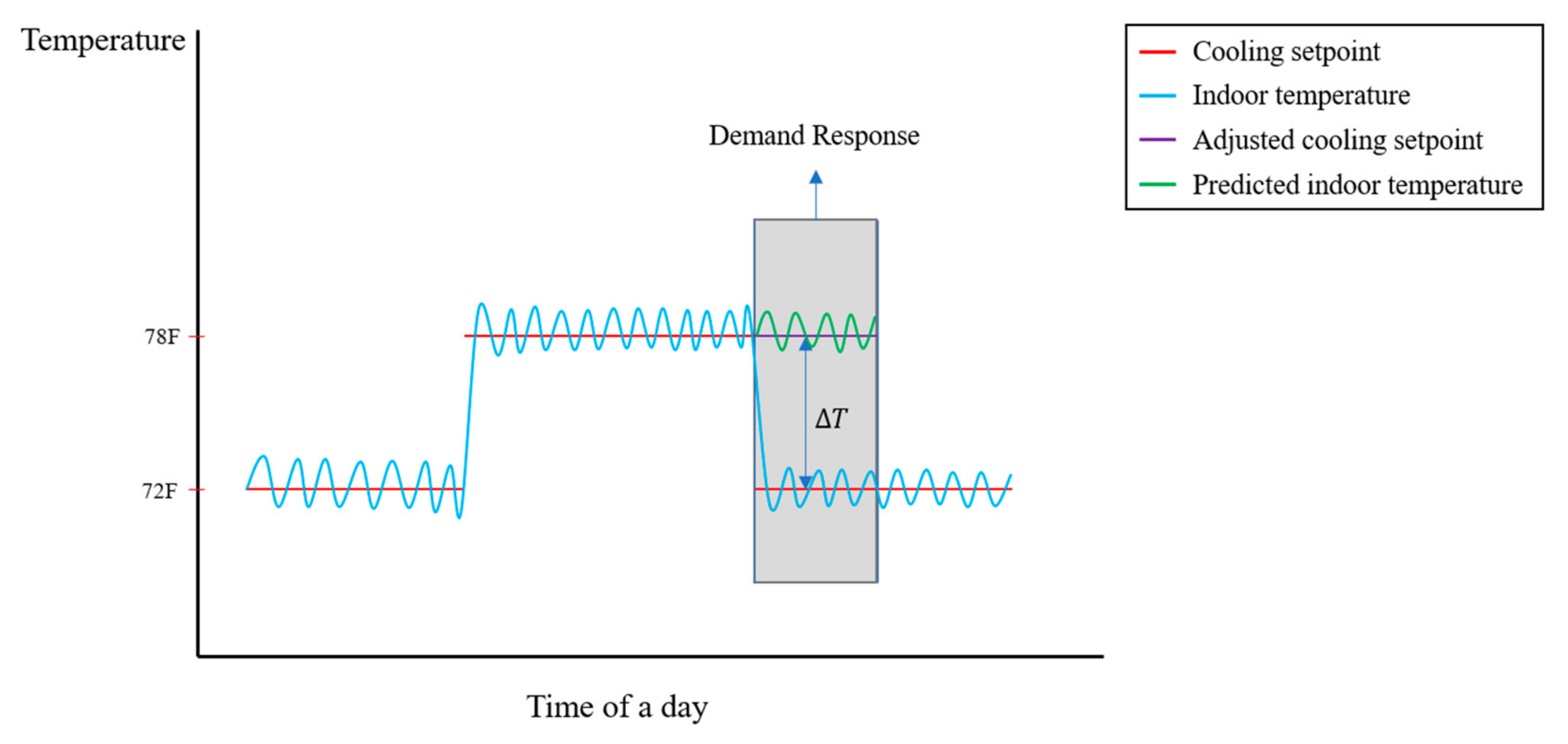
In this what-if test, the cooling status is set to off during a period of set point increase to simulate a demand response event as shown in Figure 5. It is assumed that the grey region in Figure 4 is the high peak demand of a day, during which time the thermostat is set to a resident minimum comfort condition (set to 78 °F) agreed to during a utility defined demand response event. This case was actually implemented to see the response of the house temperature to a demand response event. Note that residents might have agreed to different set point temperatures during demand events. Most important for the utility is that it would be able to estimate the duration that HVAC demand that could be curtailed while insuring a minimum comfort condition.

4. Results and Discussion

The main results are separated into three sections. First, the evaluation metrics on testing data using the three different deep learning algorithms are presented. Second, the energy savings for three different cooling set point schedules for one day in the what-if analysis using the best modelling approach are presented. Third, the demand curtailment duration and associated energy savings are calculated during a high demand event when the thermostat set point is increased from a normal value to a minimum thermal comfort condition.

4.1. Model Results

As noted in the Methodology section, the first 70% of the data is used for training, 15% of the data is applied for tuning model hyperparameters and validation, and the remaining 15% of the data is reserved for testing.

Table 3. Hyper-parameter settings for three best models developed and one-time step ahead prediction evaluation metrics on testing data.

Model	# of Hidden Layers	# of Units	Timesteps	Dropout	Learning Rate	MAE	MAPE (%)
BPNN	2	128	15	0	0.001	0.639	0.8434
LSTM	1	128	30	0	0.0005	0.4803	0.6392
E-D LSTM	1	128	5	0	0.001	0.6976	0.9349

shows the hyper-parameter settings and the validation results on testing data for each of the models for the different evaluation metrics employed (MAE, MAPE, and R2) for the best models developed for the three deep learning algorithms considered. Also, the Adam optimization algorithm [25] and EarlyStopping callback technique [26] was used in three models in order to prevent overfitting problem. The results, as evidenced by the evaluation metrics shown in Table 3 (MAE and MAPE), illustrate that LSTM has the best ability to forecast indoor temperature with a good accuracy. Clear from this table is that LSTM has the lowest MAE, which means the absolute mean error between the actual temperature and predicted temperature is within 0.5, equivalent to the resolution of the thermostat temperature sensor. It is surprising that LSTM with encoder decoder structure did not improve model prediction performance. The possible reason for that is in the encoder part, when the length of input sequence is long, the information carried by the content entering first will be diluted by the information entering later. This can cause memory loss problems.

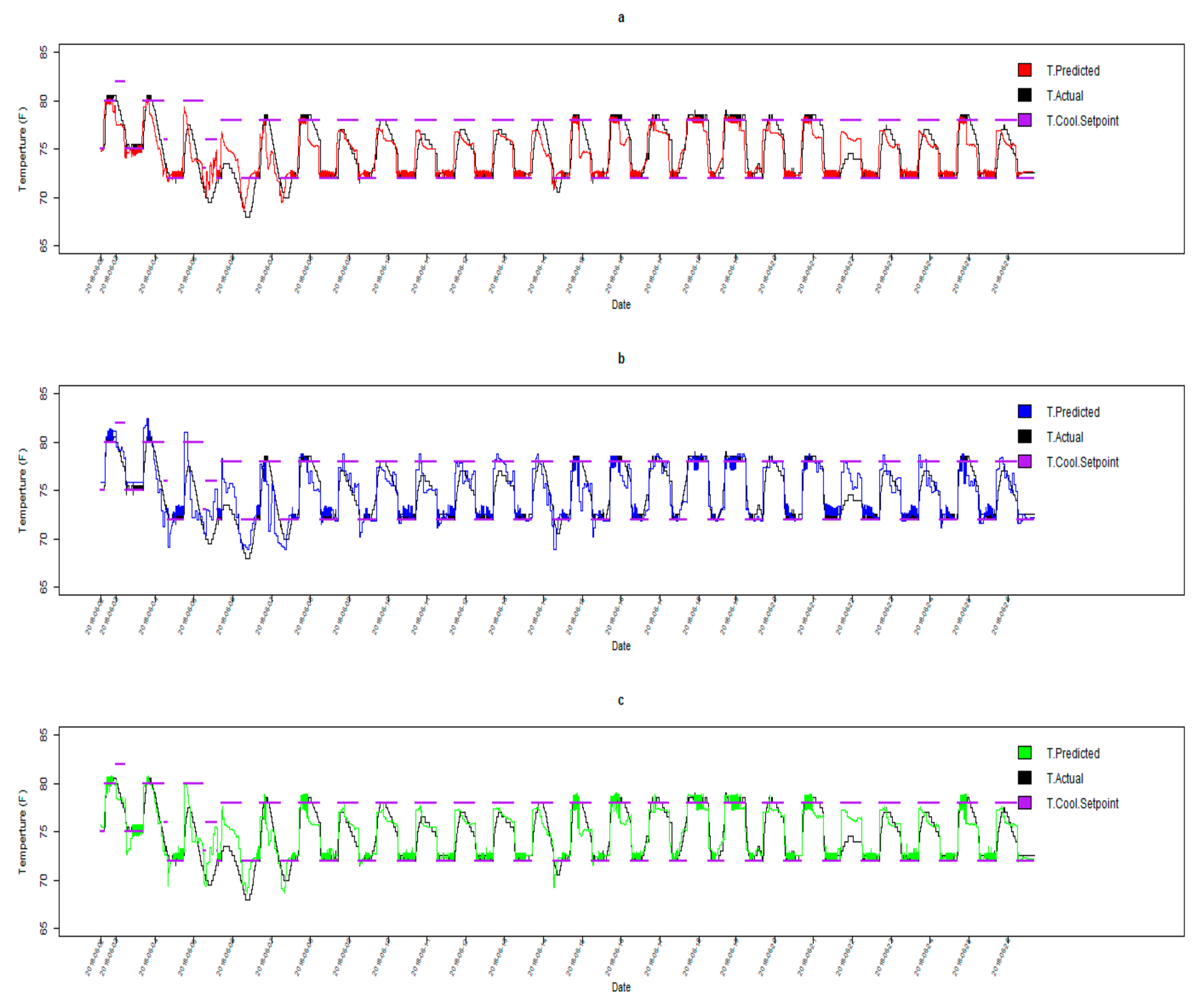
Figure 6 shows a time series of the actual and predicted temperatures on the whole dataset for respectively BPNN, LSTM (Figure 6a), and E-D LSTM. As shown in Figure 6b, the BPNN prediction of the indoor temperature does not follow the actual value when the cooling set point temperature decreases and when the cooling set point temperature is low. Likewise, in Figure 6c, it is clear that the predicted indoor temperature using the E-D LSTM approach does not exhibit the same fluctuation as for the actual value for low cooling set point temperatures. In contrast, the predictions using LSTM yields a predicted indoor temperature, which closely tracks the actual value.

4.2. What-If Analysis for Energy Saving Set Point Temperature Schedules

The what-if scenarios described in Section 3.5 were conducted using the best LSTM model, as this approach yielded the best validation performance. The control parameter (cooling status) was not known and had to be computed at each time step. The computed cooling status value was used as next time step input along with other known features (outdoor temperature and cooling set point temperature) to predict the indoor temperature at the next time step. The cooling status in the what-if simulations was calculated using the predicted indoor temperature by the following equation:

$$\mathrm{Cooling} \mathrm{status}=\left\{\begin{array}{ll}100,& |if Tindoor > Tsetpoint+0.5 \left(°F\right) \\ 0,& |if Tindoor \le Tsetpoint \end{array}\right.$$

(11)

where 0.5 (°F) is the resolution of the thermostat temperature sensor and factory control setting of the smart WiFi thermostat.

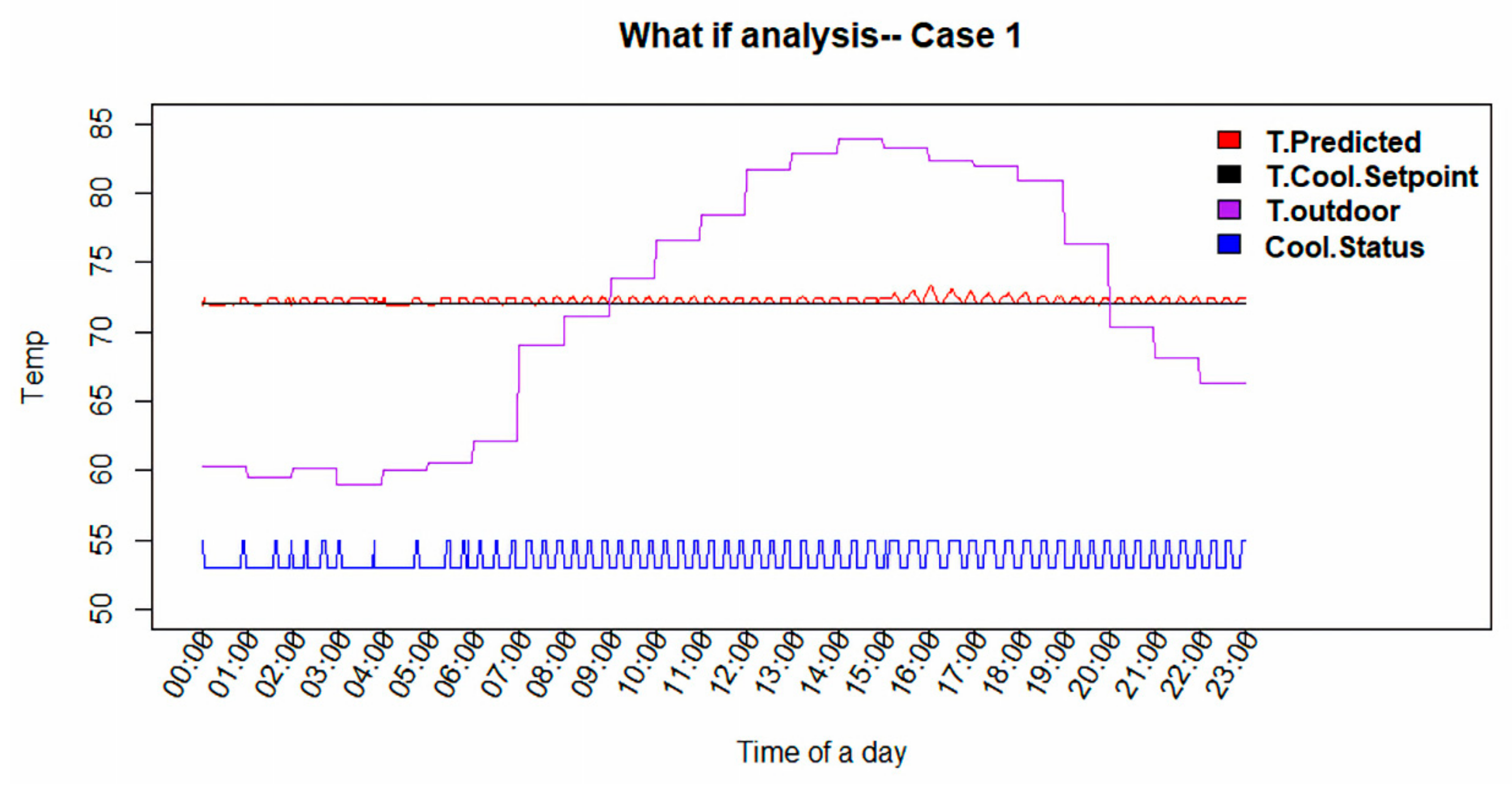
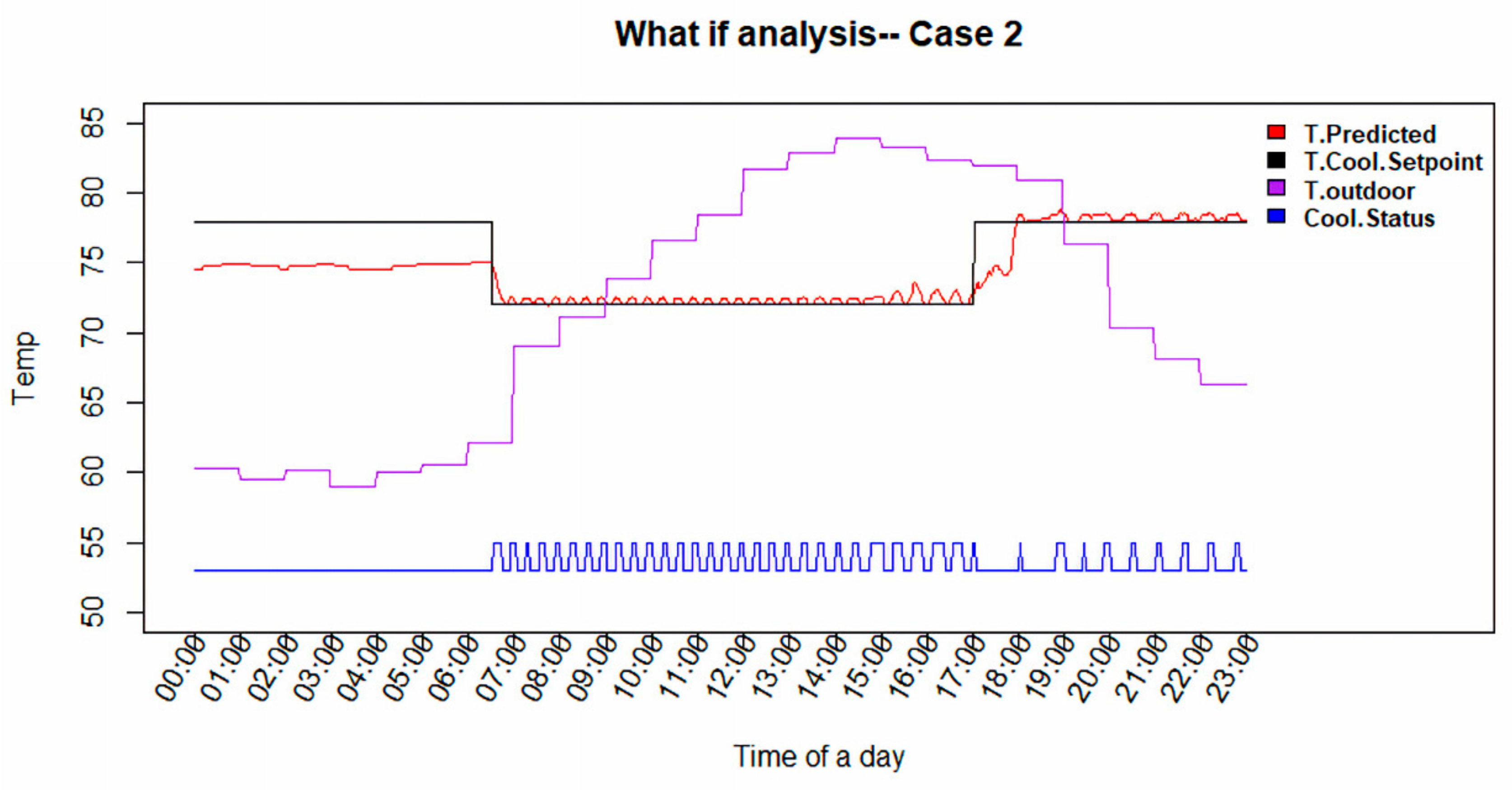
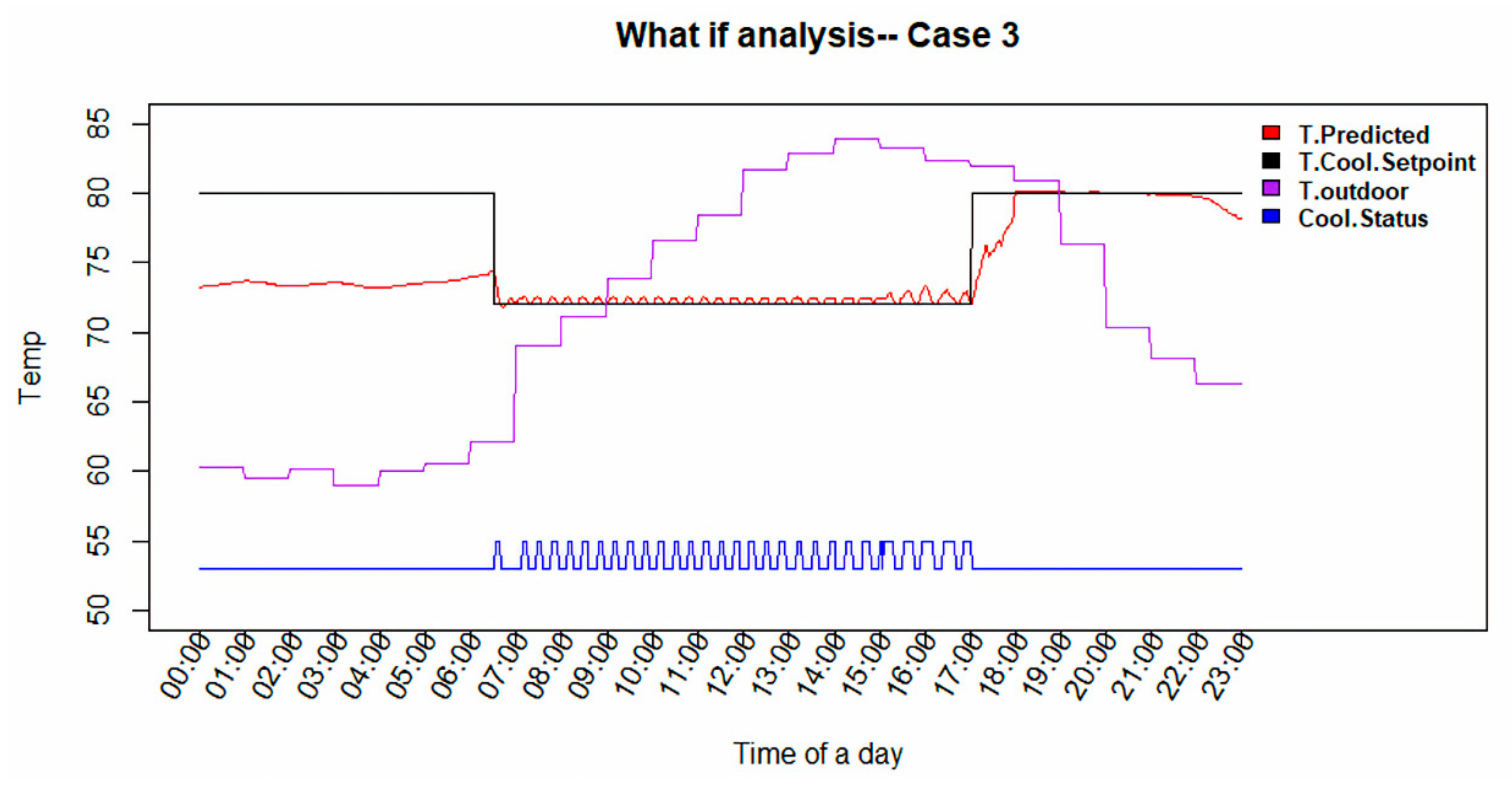
Figure 7, Figure 8 and Figure 9 show the predicted indoor temperature and computed cooling status with the same exterior temperature for three cases of what if cooling set point temperature schedules. Figure 7 shows the predicted indoor temperature, computed cooling status, and exterior temperature for the constant cooling temperature set point schedule associated with Case 1. Figure 8 shows the same parameters for a higher cooling setpoint temperature during unoccupied periods. In this figure, it is clear that the cooling duty cycle has been reduced. Lastly, Figure 9 shows results from a more aggressive cooling setpoint temperature during unoccupied periods. Again, there is a significant reduction in the cooling duty cycle.

The savings from Cases 2 and 3 can be assessed from a comparison of the predicted cooling duty cycle to the base case defined by the constant thermostat set point (Case 1), where the effective cooling duty cycle is defined as:

$$\mathrm{effective} \mathrm{duty} \mathrm{cycle} = \frac{\sum \left(Cooling time\right) \times \left(\frac{Cooling status}{100}\right)}{\sum Time}$$

(12)

Table 4. Results for the what if analysis cases considered.

Case	Total Time of a Day when Cooling Status is ON (min)	Effective Duty Cycle (%)	Cooling Energy Saving (%)
Case 1	474	32.9	-
Case 2	342	23.8	9.1
Case 3	268	18.6	14.3

summarizes the what if analysis results. Included in this table are the total time in a day when cooling status is on, effective duty cycle, and cooling energy savings for each of the cases relative to the baseline case with constant set point temperature. It is obvious that case 2 requires a lower effective cycle than the baseline case with a cooling energy reduction of 9.1%. There is more improvement in case 3, with a cooling energy reduction of 14.3% relative to the baseline case. Interestingly, one paper mentions an average of 29% cooling energy savings for a 5-degree Fahrenheit constant increase in cooling set point temperature [27]. Here, the average daily increase in set point temperature in Case 3 is 4.67 °F, less than the blanket result. Cycling of the set point temperature almost certainly will not yield as large of savings. Moreover, the savings realized will certainly depend upon the specific dynamics of a residence.

4.3. What-If Analysis for Minimum Thermal Comfort Demand Response

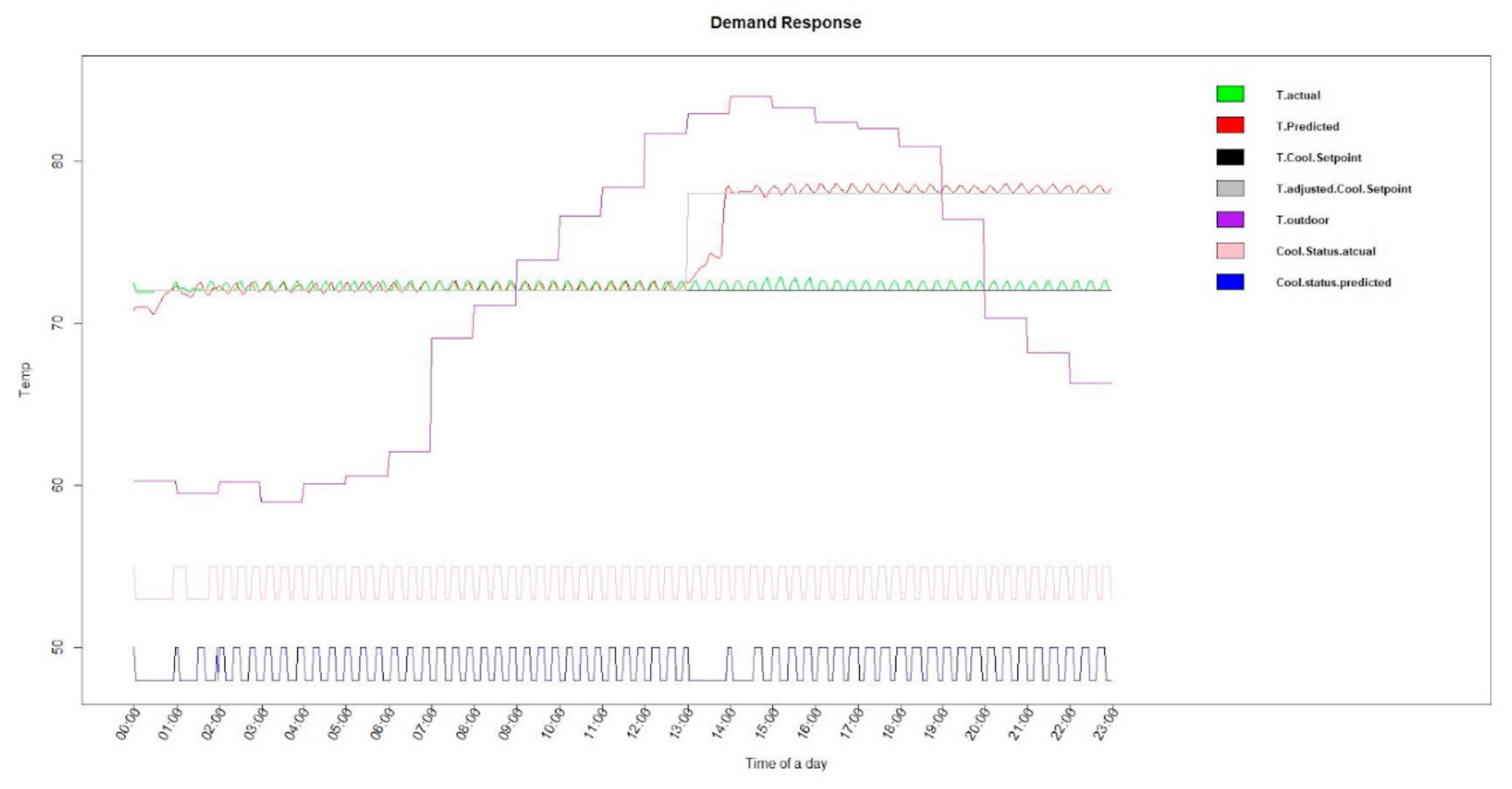
Figure 10 shows a time series response for the what if analysis for demand response for one day. Included in this figure are the actual indoor and outdoor temperatures, predicted indoor temperature, actual cooling set point temperature, an adjusted cooling set point representing corresponding to minimum thermal comfort condition, and actual cooling status and predicted cooling status during the demand reduction event. In the case shown, the cooling set point is increased from 72–78 °F at 13:00, the beginning of a simulated demand reduction event. The higher temperature is the presumed minimum comfort condition, which would be pre-determined by a resident. It is clear that in this case, increasing the cooling set point by 5 °F during the high peak demand event permitted interruption of the cooling system for about an hour given the weather conditions. This demand reduction could be communicated to the utility by the thermostat manager and the resident would receive a financial benefit from the utility for permitting curtailment.

5. Conclusions

In this research, smart Wifi thermostat data have been shown to be invaluable for developing dynamic models of the thermal comfort of a residence. An LSTM-NN approach was shown to be the best algorithm for predicting next time step forecasts for indoor temperature. The implications of this research are two-fold. First, the dynamic model created for any residence can be used to guide residents about the energy savings derivable from set point schedule changes. Second, the developed dynamic model can be used to estimate the duration of HVAC curtailment in any residence while maintaining minimum comfort bands during the high demand event. These residents could benefit from a lower energy cost if they agree to curtail cooling or heating in response to a grid-requested demand reduction event. Further studies will focus on adding solar radiation information into a dynamic model to seek how solar radiation affects the energy consumption of a residence and upon implementing the developed strategies at-scale.

References

- Consumption & Efficiency. 2019. Available online: https://www.eia.gov/consumption/ (accessed on 31 August 2020).
- Reyna, J.; Chester, M.V. Energy efficiency to reduce residential electricity and natural gas use under climate change. Nat. Commun. 2017, 8, 14916. [Google Scholar] [CrossRef] [PubMed]
- Thomas, B.; Soleimani-Mohseni, M. Artificial neural network models for indoor temperature prediction: Investigations in two buildings. Neural Comput. Appl. 2006, 16, 81–89. [Google Scholar] [CrossRef]
- Fan, C.; Xiao, F.; Zhao, Y. A short-term building cooling load prediction method using deep learning algorithms. Appl. Energy 2017, 195, 222–233. [Google Scholar] [CrossRef]
- Xu, C.; Chen, H.; Wang, J.; Guo, Y.; Yuan, Y. Improving prediction performance for indoor temperature in public buildings based on a novel deep learning method. Build. Environ. 2019, 148, 128–135. [Google Scholar] [CrossRef]
- Ruano, A.E.; Crispim, E.; Conceicao, E.Z.; Lúcio, M.M.J.R. Prediction of building’s temperature using neural networks models. Energy Build. 2006, 38, 682–694. [Google Scholar] [CrossRef]
- Attoue, N.; Shahrour, I.; Younes, R. Smart Building: Use of the Artificial Neural Network Approach for Indoor Temperature Forecasting. Energies 2018, 11, 395. [Google Scholar] [CrossRef]
- Yu, D.; Abhari, A.; Fung, A.S.; Raahemifar, K.; Mohammadi, F. Predicting Indoor Temperature from Smart Thermostat and Weather Forecast Data. In Proceedings of the Communications and Networking Symposium, CNS ’18, Baltimore, MA, USA, 15–18 April 2018; Society for Computer Simulation International: San Diego, CA, USA, 2018. [Google Scholar]
- Lou, R.; Hallinan, K.P.; Huang, K.; Reissman, T. Smart Wifi Thermostat-Enabled Thermal Comfort Control in Residences. Sustainability 2020, 12, 1919. [Google Scholar] [CrossRef]
- Al Tarhuni, B.; Naji, A.; Brodrick, P.G.; Hallinan, K.P.; Brecha, R.J.; Yao, Z. Large scale residential energy efficiency prioritization enabled by machine learning. Energy Effic. 2019, 12, 2055–2078. [Google Scholar] [CrossRef]
- Makridakis, S.; Wheelwright, S.; Hyndman, R.; Chang, Y. Forecasting Methods and Applications, 3rd ed.; John Wiley & Sons: New York, NY, USA, 1998. [Google Scholar]
- Lepot, M.; Aubin, J.-B.; Clemens, F. Interpolation in Time Series: An Introductive Overview of Existing Methods, Their Performance Criteria and Uncertainty Assessment. Water 2017, 9, 796. [Google Scholar] [CrossRef]
- Xu, P.; Han, S.; Huang, H.; Qin, H. Redundant features removal for unsupervised spectral feature selection algorithms: An empirical study based on nonparametric sparse feature graph. Int. J. Data Sci. Anal. 2018, 8, 77–93. [Google Scholar] [CrossRef]
- Tuv, E.; Borisov, A.; Runger, G.C.; Torkkola, K. Feature Selection with Ensembles, Artificial Variables, and Redundancy Elimination. J. Mach. Learn. Res. 2009, 10, 1341–1366. [Google Scholar]
- Allaire, J. R Studo Blog. 2017. Available online: https://blog.rstudio.com/2017/09/05/keras-for-r/ (accessed on 31 August 2020).
- Hochreiter, S.; Schmidhuber, J. Long Short-Term Memory. Neural Comput. 1997, 9, 1735–1780. [Google Scholar] [CrossRef]
- Hochreiter, S. The Vanishing Gradient Problem During Learning Recurrent Neural Nets and Problem Solutions. Int. J. Uncertain. Fuzziness Knowl. Based Syst. 1998, 6, 107–116. [Google Scholar] [CrossRef]
- Cho, K.; Van Merrienboer, B.; Gulcehre, C.; Bahdanau, D.; Bougares, F.; Schwenk, H.; Bengio, Y. Learning Phrase Representations using RNN Encoder–Decoder for Statistical Machine Translation. In Proceedings of the 2014 Conference on Empirical Methods in Natural Language Processing (EMNLP); Association for Computational Linguistics (ACL): Stroudsburg, PA, USA, 2014; pp. 1724–1734. [Google Scholar]
- Wu, Y.; Schuster, M.; Chen, Z.; Le, Q.V.; Norouzi, M.; Macherey, W.; Krikun, M.; Cao, Y.; Gao, Q.; Macherey, K. Google’s Neural Machine Translation System: Bridging the Gap between Human and Machine Translation. arXiv 2016, arXiv:1609.08144. [Google Scholar]
- Sutskever, I.; Vinyals, O.; Le, Q. Sequence to Squence Learning with Neural Networks. In Advances in Neural Information Processing Systems; MIT Press: Cambridge, MA, USA, 2014; pp. 3104–3112. [Google Scholar]
- Liang, L.; Xingxing, Z.; Kyunghyun, C.; Steve, R. A study of the Recurrent Neural Network Encoder-Decoder for Large Vocabulary Speech Recognition. In Proceedings of the Annual Conference of the International Speech Communication Association, INTERSPEECH, Dresden, Germany, 6–10 September 2015. [Google Scholar]
- Ou, W.; Chen, C.; Ren, J. T2S: An Encoder-Decoder Model for Topic-Based Natural Language Generation. In Bioinformatics Research and Applications; Springer Science and Business Media LLC: Cham, Switzerland, 2018; pp. 143–151. [Google Scholar]
- Akram, M.; El, C. Sequence to Sequence Weather Forecasting with Long Short-Term Memory Recurrent Neural Networks. Int. J. Comput. Appl. 2016, 143, 7–11. [Google Scholar] [CrossRef]
- Rizzi, S.; Mankovskii, S.; Van Steen, M.; Garofalakis, M.; Fekete, A.; Jensen, C.S.; Snodgrass, R.T.; Wun, A.; Josifovski, V.; Broder, A.; et al. What-If Analysis. In Encyclopedia of Database Systems; Springer: Berlin, Germany, 2009; pp. 3525–3529. [Google Scholar]
- Kingma, P.D.; Ba, J. Adam: A Method for Stochastic Optimization. arXiv 2014, arXiv:1412.6980. [Google Scholar]
- Caruana, R.; Lawrence, S.; Giles, C. Overfitting in Neural Nets: Backpropagation, Conjugate Gradient, and Early Stopping. In Advances in Neural Information Processing Systems; MIT Press: Cambridge, MA, USA, 2000; Volume 13. [Google Scholar]
- Hoyt, T.; Arens, E.; Zhang, H. Extending air temperature setpoints: Simulated energy savings and design considerations for new and retrofit buildings. Build. Environ. 2015, 88, 89–96. [Google Scholar] [CrossRef]
© 2020 by the authors. Licensee MDPI, Basel, Switzerland. This article is an open access article distributed under the terms and conditions of the Creative Commons Attribution (CC BY) license (http://creativecommons.org/licenses/by/4.0/).