Abstract
At present, the recognition of vehicle flow is mainly achieved with an artificial statistical method or by intelligent recognition based on video. The artificial method requires a large amount of manpower and time, and the existing video-based vehicle flow recognition methods are only applicable to straight roads. Therefore, a deep recognition model (DERD) for urban road vehicle flow is proposed in this paper. Learning from the characteristic that the cosine distance between the feature vectors of the same target in different states is in a fixed range, we designed a deep feature network model (D-CNN) to extract the feature vectors of all vehicles in the traffic flow and to intelligently determine the real-time statistics of vehicle flow based on the change of distance between vectors. A detection and tracking model was built to ensure the stability of the feature vector extraction process and to obtain the behavior trajectory of the vehicle. Finally, we combined the behavior and the number of vehicle flows to achieve the deep recognition of vehicle flow. After testing with videos recorded in actual scenes, the experimental results showed that our method can intelligently achieve the deep recognition of urban road vehicle flow. Compared with the existing methods, our approach shows higher accuracy and faster real-time performance.
1. Introduction
A rapid increase in car ownership has aggravated traffic pressure in cities. On urban roads, traffic jams, an unreasonable control of traffic lights, and many other traffic phenomena often occur. In order to solve these traffic problems, intelligent transportation systems (ITSs) and intelligent traffic surveillance systems (ITSSs) have been proposed [1,2]. In the past 10 years, ITS and ITSS have made great achievements in the field of traffic [3,4,5], showing that intelligent transportation is an inevitable trend in the development of human society and an important technological revolution in the future. As an important part of ITS and ITSS, research into vehicle flow is of great significance to the promotion of the development of intelligent transportation. There are currently two main avenues of research into vehicle flow: the short-term prediction of target road vehicle flow and video-based vehicle flow intelligent statistics. The former requires a large amount of manpower and material resources in the process of collecting vehicle flow data, while the latter approach is based on straight roads as the research object. The results have larger errors when applied to complex environments.
The research into the short-term prediction of vehicle flow is currently exhibiting rapid development. Li et al. acquired vehicle flow data through offline collection and then processed the acquired flow data in advance, selected the data suitable for their experimental requirements, and finally used a hybrid model combining support vector regression (SVR) and autoregressive integrated moving average (ARIMA) to achieve short-term prediction of vehicle flow on a target road [6]. Liu et al. combined the SVR model with the k-nearest neighbor (KNN) algorithm to propose a new KNN–SVR traffic flow prediction model [7]. The rapid development of deep learning has been tremendously convenient for the development of the transportation field. Ma et al. combined the restricted Boltzmann machine (RBM) with the recurrent neural network (RNN) to construct a short-term traffic flow prediction model [8]. Deng et al. used the convolutional neural network (CNN) to make short-term predictions of the vehicle flow of a target road [9]. Although the above research methods are able to make short-term predictions of the future vehicle flow on a target road through certain models, the accuracy of all results must depend on the accuracy of the collected vehicle flow data, and this requires a great deal of manpower and material resources in the process of collecting vehicle flow data. In this type of research, the method of collecting vehicle flow data is usually to install detection equipment on the target road in advance and collect information regarding vehicles passing along the road [10], and then to analyze the statistics of the collected information according to artificial methods [11]. However, these methods collect vehicle flow data in a single direction; when dealing with complex environments such as urban crossroads, there are often repeated statistics. In urban roads, vehicle flow is a dynamic process of change, with non-linearity and spatial–temporal variation [12]. Therefore, the real-time recognition of vehicle flow would be preferable. The adoption of intelligent methods to recognize the actual traffic conditions on urban roads in real time is a difficult problem in the development of ITS.
With the rapid development of visual detection algorithms, it is possible to realize this intelligent approach, and video-based vehicle flow recognition has begun to develop rapidly [13]. Based on video images, detection-tracking statistics of moving vehicles have been analyzed to achieve vehicle flow recognition. Peng S. and Ling G. et al. adopted a visual detection algorithm, first setting the region of interest (ROI) in the video image and then detecting the state of a vehicle passing through the ROI to achieve the recognition of vehicle flow [14,15]. Yingqin X.; Shiva K.; and Jiajia Y. et al. first set up a virtual detection line or ROI in the video image and then used the visual detection algorithm to judge the position of the vehicle detection bounding box and virtual detection line or ROI, thus achieving the recognition of vehicle flow [16,17,18]. However, this type of visual detection algorithm has higher requirements regarding the lighting conditions of the video, and its detection accuracy is relatively low. With the rapid development of deep learning, visual detection algorithms based on deep learning have shown good results in terms of accuracy and real-time performance. Girshick et al. proposed the R-CNN detection algorithm, which uses CNN to extract target features, but the training steps of this model are more cumbersome [19]. In order to improve these defects of R-CNN, faster RCNN has been proposed [20]. Although the detection accuracy and operation speed are improved by this method, real-time detection cannot be achieved for some complex scenarios. In order to improve the accuracy of detection algorithms, researchers have begun to combine detection and tracking. Liu et al. used a neural network-based target detection algorithm and Kalman filter algorithm to achieve vehicle detection and tracking [21]. Wu et al. proposed an improved, fast, online multi-target track method and established an adaptive track mechanism [22]. Henriques J.F et al. used the kernel correlation filter track algorithm to achieve the continuous tracking of multi-motion targets, which showed good track stability [23]. With the development of tracking algorithms, the combination of detection and tracking has begun to be introduced into video-based vehicle flow detection. Liu et al. used the yolov1 detection model and mean shift tracking algorithm to detect and track vehicles in the ROI to achieve vehicle flow recognition [24]. Bouvie C. et al. combined the visual detection algorithm with the particle filter tracking algorithm and achieved vehicle flow recognition by detecting and tracking the vehicles in the target area [25]. Muhamad S. et al. combined the visual detection algorithm with the Hungarian tracking algorithm to detect and track vehicles in the video by counting the number of times a vehicle crosses the virtual counting line; thus, traffic flow recognition was achieved [26]. However, these existing video-based vehicle flow recognition methods are only applicable to straight roads and for complex scenes, such as intersections, the results exhibited high errors. Meanwhile, when the tracking target is blocked, tracking failure occurs in these models, which causes errors in the vehicle flow statistics results. However, in urban roads, the block phenomenon is common; therefore, it is necessary to construct an appropriate model to accurately recognize the vehicle flow.
In order to intelligently obtain accurate statistics of the vehicle flow on urban roads, this paper is based on the Cosine distance metric [27]. For different feature vectors, the directionality is more important than the value and the traditional Euclidean distance metric is only sensitive to the value [28], and does not use the directionality between the feature vectors. Compared with the Euclidean distance metric, the Cosine distance metric pays more attention to the difference in the direction. At present, the cosine metric is mainly used in the field of person re-identification (Re-ID) [29].
Based on deep learning, this paper first constructs a detection model (DEM) to detect vehicles on the road. In order to ensure the detection stability of vehicles in the process of motion, a behavior tracking model (TRM) is constructed to continuously track the movement process of the vehicle, and to continuously extract the movement behavior information of the vehicle, as well as to display the movement behavior of vehicles with the trajectory. Next, a feature extraction network (D-CNN) is constructed to extract the feature vector of the vehicle. Finally, the cosine distance change is used between vectors to intelligently achieve the real-time statistics of vehicle flow and trajectory behavior. The number of vehicle flow are combined to achieve in-depth recognition of vehicle flow. Finally, we experiment with our method through actual road videos.
2. Methods
In order to solve the shortcomings of existing vehicle flow recognition methods, we proposed a deep recognition model (DERD) of vehicle flow based on deep learning. Based on surveillance video, a method that combines detection-tracking-feature vector and extraction-statistics of vehicles on the road was carried out to achieve the deep recognition of vehicle flow. The model mainly includes vehicle flow information extraction module (DEM), behavior tracking module (TRM), and flow statistics module (STM). The overall structure is shown in Figure 1. FEL is the detection status of the vehicle, are status parameters, are conditional parameters, is the behavior trajectory of the vehicle, TEL is the tracking status of the vehicle. DCNN is a deep feature extraction network. RA(r1, …, rn) is the feature vector of the vehicle, Q and M are the number of vehicle flow.
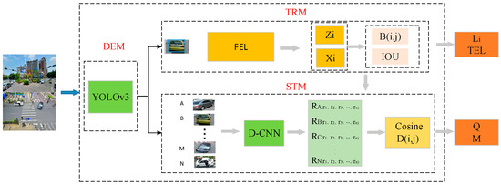
Figure 1.
The overall structure of the deep recognition model (DERD) model.
2.1. Vehicle Flow Information Extraction Module (DEM)
The vehicle flow information extraction module is equivalent to the human visual system, which can quickly locate and recognize vehicles on the road. It takes the video picture as input and the vehicle’s detection status, FEL, as output. We built the vehicle flow information extraction module based on the YOLOv3 network [30]. However, due to the classification requirements of the original YOLOv3 model, the loss function consisted of three parts. However, in the process of vehicle flow recognition, detection targets can be divided into one category, so we modified the loss function of the YOLOv3 to build a loss function suitable for us. Therefore, the model can better serve the detection of vehicle flow information. Figure 2 is a schematic diagram of the principle of the DEM module.
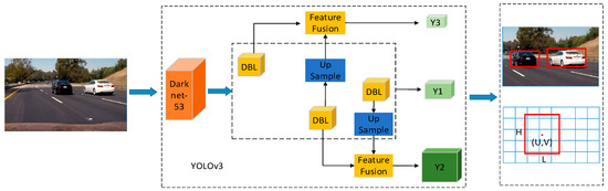
Figure 2.
Schematic diagram of the principle of vehicle flow information extraction module.
The vehicle flow information extraction module is mainly composed of Darknet-53 feature extraction network, DBL network, multi-scale fusion feature network, and more. Darknet-53 is the backbone network and is mainly composed of 53 convolutional layers, using a large number of 3 × 3, 1 × 1 convolutions kernels. It constructs residual blocks between convolutional layers and creates short-cut connections. There is no pooling layer and fully connected layer that accelerates the network operations. YOLOv3 generates three different scale features (Y1, Y2, Y3) for the detected target and each feature has three different candidate boxes in size. Finally, according to the confidence requirements, the most accurate candidate box was selected as the actual detection bounding box of the detected target and the detection state FEL (center coordinate and width and height) of the target was the output.
The loss function of YOLOv3 is composed of three parts, i.e.; bounding box loss, confidence loss, and category loss. However, in our DERD model, the loss function of the vehicle flow information extraction network is mainly composed of and [31,32].
2.2. Behavior Track Module (TRM)
The movement information of the vehicle on the road is continuous, so we built a behavior tracking module to ensure the stability of vehicle detection and feature vector extraction during the movement. The TRM mainly includes two parts: prediction of the vehicle motion model and detection-tracking matching. Taking the vehicle detection state FEL as input, we predicted the tracking state of the vehicle based on the motion model and then matched the predicted tracking state of the vehicle with the actual detection state to achieve continuous vehicle tracking. The output of the TRM module is the actual tracking state TEL and trajectory of the vehicle. The continuous tracking process of the vehicle is shown in Figure 3.
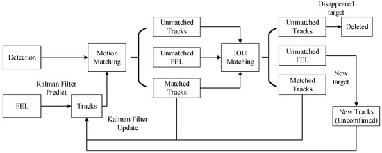
Figure 3.
Flow chart of continuous vehicle tracking.
The motion trajectory of the vehicle is a sequence of its centroid coordinates connected at different times during the motion of the image plane. The trajectory is represented by Equation (1).
is the coordinate and frame number of the vehicle in the image plane when the tracking module (TRM) tracks the vehicle for the i-th time.
2.2.1. Vehicle Motion Model Prediction
On urban roads, vehicles usually travel at low speeds. In video images, the position of the vehicle changes slightly between video sequences. Therefore, this paper assumes that the vehicle’s motion process is linearly related, which system satisfies Equations (2)–(4).
are the tracking state of the vehicle at the i-th and (i−1)-th frames, respectively; is the vehicle detection state at the i-th frame; are the state parameter matrices of the system; are the process noise and detection noise of the i-th frame in the process of vehicle tracking and detection, respectively; represent the center position, area, and aspect ratio of the track bounding box.
Assuming that follow the Gaussian distribution and their covariance matrices are , respectively, the entire motion model is divided into prediction and update.
(1) Prediction part: The same target vehicle is detected in three consecutive frames, which means that the target vehicle is not a false detection vehicle. It is necessary to predict the track state and its covariance matrix based on the detection state, as shown in Equations (5) and (6).
is the i-th predicted frame of vehicle tracking state based on the i−1th frame of the vehicle tracking state. is the covariance matrix of and is the covariance matrix of .
(2) Update part: After the detection state and tracking state of the target vehicle are successfully matched in the system, the tracking state of the vehicle and its covariance matrix needs to be continuously updated in every frame, as shown in Equations (7)–(9).
is the covariance matrix of ; is the Kalman gain of the frame .
2.2.2. Detection and Tracking Matching
On urban roads, the occlusion phenomenon often occurs when the vehicle is moving. In order to achieve the detection and tracking when the vehicle is occluded, we adopted two methods: motion position matching based on the Mahalanobis distance and Intersection over Union (IOU) matching based on the Hungarian algorithm. The matching state is divided into two types: verified and unverified.
First, the matching relationship of movement position is established and the Mahalanobis distance between the predicted tracking state and the detection state of the vehicle is calculated, as shown in Equations (10) and (11).
is the covariance matrix between and , and is the threshold determined in the experiment. When Equations (11) and (12) are satisfied, the matching is considered successful and the goal is in the state of being confirmed.
IOU matching based on the Hungarian algorithm is performed for the vehicles whose matching status has not been determined after the motion position matching.
To establish the IOU matching relationship, the IOU value between the vehicle detection bounding box and the tracking bounding box is calculated, as shown in Equations (12) and (13).
Q represents the number of all detection targets, i (); is the threshold determined in the experiment to ensure that some match results with low correlation are deleted.
2.3. Flow Statistics Module (STM)
The flow statistics module intelligently achieves the real-time statistics of the vehicle flow based on the changes in the distance between the feature vectors of the vehicles [33]. In order to accurately and quickly extract the feature vectors of vehicles in urban roads, we construct a deep feature extraction network (D-CNN). Its structure is shown in Figure 4.
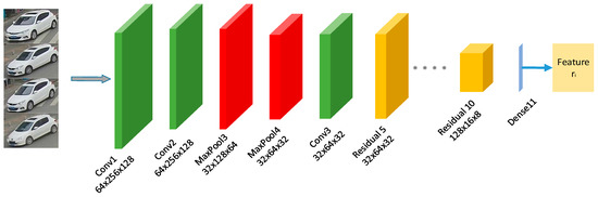
Figure 4.
Deep feature network model (D-CNN).
The deep feature network is mainly composed of convolutional layers, pooling layers, and residual blocks [34]. Each residual block contains two convolutional layers. As shown in Figure 4, the layers in the network structure is named according to their category and their order in the entire deep feature network. For example, Conv1 represents the first convolutional layer in the deep feature network and Residual 5 indicates that the fifth layer in the deep feature network is a residual block. The feature network contains 5 residual blocks. Firstly, the input image is scaled to 256 × 128 and transmitted to the network’s convolutional layer in Red as Integer, Green as Integer, Blue as Integer (RGB) format. First, the features extraction of the whole range of the detected image with Conv1 is started and the output are 64 × 256 × 128. The output features are then subjected to two more consecutive pool layer operations to perform more specific sample process on the feature and the pooled feature is then processed by a convolutional layer. The outputs have 32 × 64 × 32 features and the Sigmoid function is used as the activation function of all layers. The output features are continuously processed with 5 residual blocks and the structure of the residual block is shown in Figure 5, where is the input, is the expected output, is the linear rectification function, is the learning objective, and an identity mapping is added to convert the original learned function to . By introducing the residual blocks, the degradation problem caused by the increase of the number of network layers could be solved and its training error is lower than other networks with the same number of layers. The input features are processed through a series of convolutional layers and pool layers to reduce the size of the feature map to 16 × 8. Finally, the dimension reduction process is performed through Dense11 (fully connected layer) to extract the global feature vector with a dimension of 128.
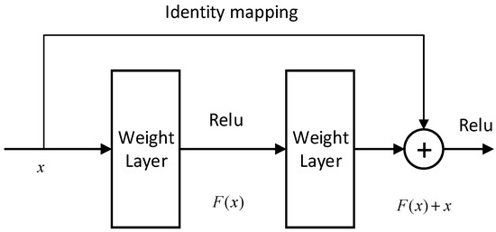
Figure 5.
Residual block.
The loss function of D-CNN is mainly composed of the predicted category value and the true category value between the feature vectors, as shown in Equations (14).
First, the feature vectors ( extracted by D-CNN are regularized to meet . Meantime, a feature set is created for each target that is successfully tracked and matched, and the latest 100 frames are saved. Finally, calculate the minimum cosine distance between the feature vector set of the i-th tracking target vehicle and the j-th detection target vehicle in the current frame, as shown in Equations (15) and (16).
is the unit feature vector of the j-th detection target. represents any feature vector of the i-th track target feature set. is the threshold determined in the experiment. When Equations (15) and (16) are satisfied, it is considered that the detected vehicle and the tracked vehicle are the same target, and no new target appears in the current field of view; thus, vehicle ID will not change. According to the ID number of detected-tracked vehicles on the road, the real-time statistics (M) of the current vehicle flow on the road is achieved. When Equations (15) and (16) are not satisfied for three consecutive frames, it is considered that a new target appears. Then, a new ID is assigned to the target and the statistical of the total vehicle flow (Q) through the road increases by one.
2.4. Detail
2.4.1. Data Set Description
In our DERD model, our data set contained two parts: a DEM data set and D-CNN model data set. The data set of the DEM model includes: Pascal VOC2007, a part of the vehicle pictures from Pascal VOC201, and a self-recorded road traffic video at Yanta Road in Xi’an. Then, the video was processed into a single-frame image through python and 15,000 pictures in VOC format data set were made by LableImg. Each picture in the VOC format data set had a corresponding label file, which gave the bounding box and class label of the objects appearing in the picture. The data set had a total of 21,000 pictures, as shown in Figure 6a.
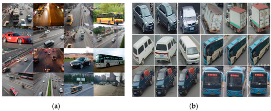
Figure 6.
Example of sample set: (a) is an example of the DEM part of the training data set; (b) is an example of the D-CNN part of the training data set.
The data set of the deep feature network (D-CNN) included a total of 10,000 pictures of the vehicle pictures in the vehicle recognition data set VeRi776 [35], as shown in Figure 6b. The data set images in VeRi776 were captured in real-world unconstrained surveillance scenes and marked with different attributes, such as type, color, and brand. Each car was photographed by multiple cameras under different viewpoints, lighting, resolution, and occlusion. It also marked enough license plate and space-time information, such as the BBox of the plate, the license plate number, the shooting time, and the distance between adjacent cameras.
2.4.2. Model Training
In our DERD model, the training of the network model mainly included DEM and D-CNN. We show our process from the setting of training parameters and training results, respectively.
The training network parameter settings are as follows. When training the DEM network model and the D-CNN model, we need to set the relevant parameters according to our experimental requirements. The training parameters are shown in Table 1a,b, respectively.

Table 1.
Training parameters.
Figure 7 shows the training process of the DEM model and D-CNN training. It can be seen from Figure 7a that the loss of the DEM network model dropped to about 15% after 350 epochs and then it started to converge. As shown in Figure 7b, it can be seen that the loss of D-CNN dropped faster before 50,000 steps, whereas it started to decline steadily after 50,000 steps. When it reached 350,000 steps, the model tended to converge.
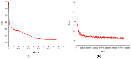
Figure 7.
Training process diagram: (a) is the loss training process of DEM network; (b) is the loss training process of D-CNN.
In our DERD model, we chose the parameters to combine the actual experimental effect with the pedestrian multi-target tracking [36] model and finally confirmed . In the selection process of parameter , the size of determines whether the feature vectors of different vehicles can achieve accurate classification and the accuracy of traffic flow statistics. We conducted an experimental test on the correspondence between the value of the threshold and the classification accuracy . The result is shown in Figure 8. From the experimental result, we can see that when , the classification accuracy had a rapid drop. was set as 0.6 in our DERD model.
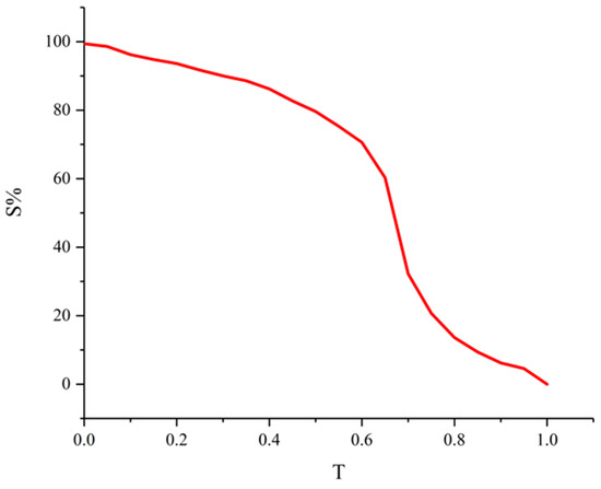
Figure 8.
Classification accuracy change chart.
3. Experimental Results and Analysis
First, we compared the performance of the trained detection model (DEM), RCNN [19], faster RCNN [20], a detection model [24], and the YOLOv3 [30] model for vehicle detection. Taking the visual detection algorithm performance evaluation index mAP% (average accuracy rate), recall% (recall rate), and FPS as reference standards, we tested it in our test data set. The results are shown in Table 2.
Table 2.
Comparison results of vehicle detection effects of different models.
It can be seen from Table 2 that our DEM model shows the highest accuracy rate for vehicle detection and the fastest detection speed. Compared with YOLOv3, although the vehicle detection accuracy only increased by 0.002, the FPS increased from 15.71 to 16.87.
In an urban road traffic scene, the real-time detection of vehicle flow played an important role in the adjustment of signal lights, emergency rescue, and solving the problem of traffic congestion. In order to verify the accuracy and real-time performance of our DERD model on the recognition of vehicle flow on urban roads, we recorded multiple sets of videos on different roads for experiments. Firstly, we compared the recognition effect of the DERD model and the traditional vehicle flow recognition model. Secondly, we conducted an experimental analysis on the stability of the vehicle flow recognition process. Finally, we conducted experimental tests on the DERD model from different scenes such as roads with smooth traffic and congested roads.
Figure 9 shows the effect of our experiment. In the output, we directly showed the number (M) of vehicles currently driven on the road, which can provide data reference for judging the degree of congestion on the road. Meanwhile, we also showed the number (Q) of all vehicles passed on the road. Secondly, we directly showed the detection effect and behavior tracking effect (FEL, TEL) of vehicles in the current traffic flow, as well as the behavior change trend of vehicles at the road (). As shown in Figure 9, in the real-time DERD model, each vehicle had a fixed ID attribute when passing through the road. The white bounding box was the detection status (FEL) of the vehicle and the colored bounding box was the behavior tracking status (TEL) of the vehicle.
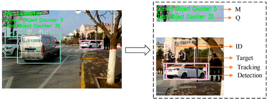
Figure 9.
Experimental effect display.
As shown in Figure 10b, the area inside the black bounding box was the ROI. In Figure 10c, the red line was the vehicle flow counting line. It can be seen from Figure 10 that our method had a more obvious advantage on road vehicle recognition. Compared with the existing methods based on the ROI model and counting line model, our method not only counted all the vehicles that passed on the road, but also accurately counted the vehicles driving on the road. Compared with existing methods, our method showed the fastest recognition speed.
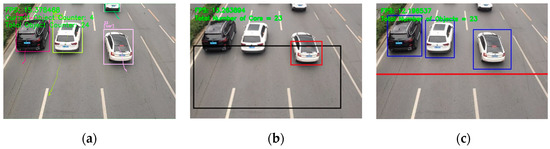
Figure 10.
The comparison graph of different model test results. (a–c) respectively represent the experimental results of the DERD, ROI model [22], and counting line model [24].
Figure 11 is an experimental diagram of the stability of the DERD model in actual scenes. Figure 11 shows the vehicle detection and tracking effect of our method when the vehicle was occluded. It can be seen from the Figure 11a that the vehicle with ID 24 was blocked in a large area and the DERD model correctly tracked the behavior of the vehicle. It can be seen from Figure 11b that the vehicle with ID 24 was almost completely occluded, but the DERD model still accurately detected and tracked the vehicle. Figure 10 shows the process of the vehicle with ID 24 being blocked to leave the crossroad. In such an instance, the DERD model achieved a good tracking result on the movement of the vehicle. There was no failure to extract the feature vector of the vehicle because the vehicle was occluded, which caused the ID of the vehicle to change, resulting in traffic flow statistical errors. After analysis, the DERD model had high stability in the recognition of urban road vehicle flow.
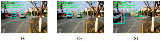
Figure 11.
Stability test experiment diagram: (a–c) shows the recognition effect at different moments.
Figure 12 is an experimental diagram of the DERD model at the scene of different straight roads. It can be clearly seen from Figure 12 that our method showed good results in the real-time recognition of vehicle flow on straight roads.
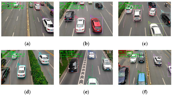
Figure 12.
Results of vehicle flow deep recognition in simple scenarios: (a–f) are different straight road scenes.
Figure 13 is an experiment diagram of vehicle flow recognition of the DERD model in a complex scene, including four different intersection scenes. Figure 13a,b show the same scene. Figure 13c,f also show the same scene. It can be seen from Figure 13 that our method not only accurately achieved the vehicle flow statistics of the intersection, but also clearly obtained the real-time vehicle flow movement trend of the intersection. From the vehicle trajectory in Figure 13e, it can be seen that some vehicles had obvious straight motion behavior, while some vehicles had no obvious motion behavior; their trajectories were in a dot state, meaning that the behavior of these vehicles mainly awaited a green light. Therefore, at this moment, there were two main traffic trends at this intersection: one went straight and the other waited for a green light. After analysis, it can be seen that the DERD model achieved a good real-time recognition result on the vehicle flow in different complex scenes and the vehicle flow in different lighting scenes. In order to verify the accuracy of the DERD model for real-time statistics of the number of intersection traffic flows, the average accuracy was selected as the evaluation indicators of DERD, as shown in the following equations.
where A is the number of vehicle flows counted by DERD and D is the number of actual vehicle flows.
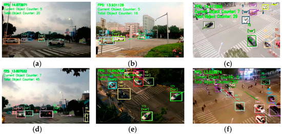
Figure 13.
Results of vehicle flow deep recognition in complex scenes: (a–f) are different complex scenes.
We took all the road videos collected (including two scenes of straight roads and intersections) as materials and compared the vehicle recognition results of the DERD model, ROI model [24], and counting line model [26]. The results are shown in Table 3.
Table 3.
Comparison of vehicle recognition results of different methods.
It can be seen from Table 3 that although the existing method showed good accuracy in the vehicle flow statistics of straight roads, the accuracy of the vehicle flow statistics was greatly reduced for the complex scene, i.e.; intersections. However, our method showed high accuracy in traffic flow statistics both on roads with little traffic and congested roads. Moreover, our method had the highest accuracy and the highest recognition speed in vehicle flow recognition on urban roads, and its real-time performance was the best.
4. Discussion
Through the experimental results and analysis, it can be seen that our DERD model shows the best results compared with the existing methods in vehicle flow recognition on urban roads. The main reasons are as follows:
(1) Existing video-based vehicle statistics models used straight roads as the research object. These models judged the number of times a vehicle passed the ROI or counting line to achieve the statistics of the vehicle flow. However, in complex scenes, the probability that the vehicle did not pass through the ROI or counting line would significantly increase, resulting in a large number of false counting phenomena. For different scenes, choosing the ROI or counting line position in the image had a great influence on the repeated counting and false counting of vehicles.
(2) Different vehicles have different feature vectors and the cosine distance between the feature vectors of different states of the same vehicle is in a fixed range. The DERD model extracted the feature vectors of all detected and tracked vehicles on the road and then used the cosine distance changes between feature vectors to achieve vehicle flow statistics, which solved the problems of false counting and repeated counting in complex scenes, so that it had the highest statistical accuracy in different scenes.
(3) We built a more accurate, faster, and more stable vehicle detection model and tracking model to improve the speed and accuracy of the traffic information extraction process, resulting in the DERD model with the fastest vehicle flow identification speed. Our method combined the vehicle behavior and the number of vehicles, showing a more intuitive vehicle flow recognition effect. Vehicles with abnormal behavior were easily judged on the basis of the trajectory flow.
However, our DERD model also has weaknesses. When vehicles with the same appearance and color appeared in the inspection field at the same time, the feature vectors extracted by the DERD model experienced a high degree of similarity, which could potentially lead to false statistics. Therefore, in future research, we will try to solve this problem.
5. Conclusions
Based on the deep learning and detecting-tracking model, this paper proposed a vehicle flow depth recognition model (DERD). Through detecting-tracking-feature extraction of vehicles, we used cosine distance as the method of vehicle statistics and made full use of the motion behavior of vehicle flow on the road. Therefore, the real-time deep recognition of vehicle flow was achieved. In the experimental section, based on the video in the actual scene, we tested the stability of the DERD model in the process of vehicle flow recognition and the recognition result of the DERD model in different scenes, and we compared it with other methods. The results showed that the DERD model not only had the highest accuracy rate for vehicle flow statistics but also intuitively showed the behavioral trend of the current vehicle flow. Compared with the existing methods, it showed the fastest recognition speed.
Author Contributions
Conceptualization, S.Z. and C.W.; investigation, C.W. and P.W.; methodology, S.Z. and C.W.; project administration, Q.Z.; resources, Q.Z.; software, S.Z.; C.W. and Q.Z.; supervision, S.Z.; validation, S.Z.; writing—original draft, C.W. and P.W.; writing—review & editing, C.W. and P.W. All authors have read and agreed to the published version of the manuscript.
Funding
This research was funded by Shaanxi Provincial Key Research and Development Program (Project No. S2020-YF-ZDCXL-ZDLGY-0295) and Shaanxi Provincial Education Department serves Local Scientific Research Plan in 2019 (Project No. 19JC028) and Shaanxi Provincial Key Research and Shaanxi province special project of technological innovation guidance (fund) (Program No. 2019QYPY-055) and the Shaanxi Province key Research and Development Program (Project No. 2019ZDLGY03-09-02) and Key Research and development plan of Shaanxi Province (Project No. S2020-YF-ZDCXL-ZDLGY-0226) and Development Program (Project No. 2018ZDCXL-G-13-9).
Conflicts of Interest
The authors declare no conflict of interest.
References
- Kalamaras, I.; Zamichos, A.; Salamanis, A.; Drosou, A.; Kehagias, D.; Papadopoulos, S.; Tzovaras, D. An interactive visual analytics platform for smart intelligent transportation systems management. IEEE Trans. Intell. Transp. Syst. 2017, 19, 487–496. [Google Scholar] [CrossRef]
- Zhang, H.; Shan, H. Research on the High Definition Intelligent Surveillance System for Urban Intersection. J. SCU 2012, 44, 224–228. [Google Scholar]
- Socha, R.; Kogut, B. Urban Video Surveillance as a Tool to Improve Security in Public Spaces. Sustainability 2020, 12, 6210. [Google Scholar] [CrossRef]
- Zhao, S.; Zhao, Q.; Bai, Y.; Li, S. A Traffic Flow Prediction Method Based on Road Crossing Vector Coding and a Bidirectional Recursive Neural Network. Electronics 2019, 8, 1006. [Google Scholar] [CrossRef]
- Zhou, W.; Wang, W.; Hua, X.; Zhang, Y. Real-Time Traffic Flow Forecasting via a Novel Method Combining Periodic-Trend Decomposition. Sustainability 2020, 12, 5891. [Google Scholar] [CrossRef]
- Li, L.; He, S.; Zhang, J.; Ran, B. Short-term highway traffic flow prediction based on a hybrid strategy considering temporal-spatial information. J. Adv. Transp. 2016, 50, 2029–2040. [Google Scholar] [CrossRef]
- Lee, C.-H.; Chih-Hung, W. A Novel Big Data Modeling Method for Improving Driving Range Estimation of EVs. IEEE Access 2015, 3, 1980–1993. [Google Scholar] [CrossRef]
- Ma, X.; Yu, H.; Wang, Y.; Wang, Y. Large-scale transportation network congestion evolution prediction using deep learning theory. PLoS ONE 2015, 10, e0119044. [Google Scholar] [CrossRef]
- Wang, Y.; Guo, Y.; Wei, Z.; Huang, Y.; Liu, X. Traffic Flow Prediction Based on Deep Neural Networks. Comput. Eng. Appl. 2019, 55, 228–235. [Google Scholar]
- Ali, S.S.M.; George, B.; Vanajakshi, L. A simple multiple loop sensor configuration for vehicle detection in an undisciplined traffic. IEEE Sens. ICSens. 2011, 10, 644–649. [Google Scholar]
- Yu, W.; Bai, H.; Chen, J.; Yan, X. Analysis of Space-Time Variation of Passenger Flow and Commuting Characteristics of Residents Using Smart Card Data of Nanjing Metro. Sustainability 2019, 11, 4989. [Google Scholar] [CrossRef]
- Sun, X.; Lin, K.; Jiao, P.; Lu, H. The Dynamical Decision Model of Intersection Congestion Based on Risk Identification. Sustainability 2020, 12, 5923. [Google Scholar] [CrossRef]
- Gruden, C.; Campisi, T.; Canale, A.; Tesoriere, G.; Sraml, M. A cross-study on video data gathering and microsimulation techniques to estimate pedestrian safety level in a confined space. In Proceedings of the IOP Conference Series Materials Science and Engineering, Prague, Czech, 18 September 2019; pp. 60301–60311. [Google Scholar]
- Peng, S. Flow detection based on traffic video image processing. J. Multimedia 2013, 8, 519–527. [Google Scholar]
- Gan, L.; Li, R. Multilane traffic flow detection algorithm based on adaptive virtual loop. J. Comput. Appl. 2016, 36, 3511–3514. [Google Scholar]
- Xie, Y.; Jiang, L.; Wang, L.; Huang, C.; Liu, T. A Fast Vehicle Detection Algorithm. J. HUST 2016, 21, 19–24. [Google Scholar]
- Kamkar, S.; Safabakhsh, R. Vehicle detection, counting and classification in various conditions. IET Intell. Transp. Syst. 2016, 10, 406–413. [Google Scholar] [CrossRef]
- Yu, J.; Zuo, M. A Video-based Method for Traffic Flow Detection of Multi-lane Road. In Proceedings of the Seventh International Conference on Measuring Technology and Mechatronics Automation, Nanchang, China, 13–14 June 2015; pp. 68–71. [Google Scholar]
- Girshick, R.; Donahue, J.; Darrell, T.; Malik, J. Rich feature hierarchies for accurate object detection and semantic segmentation. In Proceedings of the IEEE Conference on Computer Vision and Pattern Recognition, Columbus, OH, USA, 23–28 June 2014; pp. 580–587. [Google Scholar]
- Ren, S.; He, K.; Girshick, R.; Sun, J. Faster R-CNN: Towards real-time object detection with region proposal networks. IEEE Trans. Pattern Anal. Mach. Intell. 2017, 39, 1137–1149. [Google Scholar] [CrossRef]
- Liu, J.; Hou, S.; Zhang, K.; Zhang, R.; Hu, C. Vehicle real-time detection and tracking based on enhanced Tiny YOLOV3 algorithm. Trans. Chin. Soc. Agric. Eng. 2019, 35, 118–125. [Google Scholar]
- Wu, H.; Li, W. Robust online multi-object tracking based on KCF trackers and reassignment. In Proceedings of the IEEE Global Conference on Signal and Information Processing, Washington, DC, USA, 24 April 2017; pp. 124–128. [Google Scholar]
- Henriques, J.F.; Caseiro, R.; Martins, P.; Batista, J.P. High-Speed Tracking with Kernelized Correlation Filters. IEEE Trans. Pattern Anal. Mach. Intell. 2015, 37, 583–596. [Google Scholar] [CrossRef]
- Liu, L.; Zhao, S.; Guo, W. Traffic flow statistics method based on YOLO recognition and mean shift tracking. Manuf. Autom. 2020, 42, 16–20. [Google Scholar]
- Bouvie, C.; Scharcanski, J.; Barcellos, P.; Escouto, F.L. Tracking and counting vehicles in traffic video sequences using particle filtering. In Proceedings of the IEEE International Instrumentation and Measurement Technology Conference, Minneapolis, MN, USA, 6–9 May 2013; pp. 812–815. [Google Scholar]
- Soleh, M.; Jati, G.; Hilman, M.H. Multi-Object Detection and Tracking using optical flow density Hungarian Kalman Filter (OFD-HKF) Algorithm for Vehicle Counting. J. Ilmu Komput. Dan Inf. 2018, 11, 17–26. [Google Scholar] [CrossRef]
- Mikawa, K.; Ishida, T.; Goto, M. A proposal of extended cosine measure for distance metric learning in text classification. In Proceedings of the IEEE International Conference on Systems, Man, and Cybernetics, Anchorage, AK, USA, 9–12 October 2011; pp. 1741–1746. [Google Scholar]
- Elmore, K.L.; Richman, M.B. Euclidean Distance as a Similarity Metric for Principal Component Analysis. Mon. Weather Rev. 2001, 129, 540–549. [Google Scholar] [CrossRef]
- Wojke, N.; Bewley, A. Deep Cosine Metric Learning for Person Re-Identification. In Proceedings of the IEEE Winter Conference on Applications of Computer Vision, Lake Tahoe, NV, USA, 12–15 March 2018; pp. 748–756. [Google Scholar]
- Redmon, J.; Farhadi, A. Yolov3: An incremental improvement. arXiv 2018, arXiv:1804.02767. [Google Scholar]
- Redmon, J.; Divvala, S.; Girshick, R.; Farhadi, A. You only look once: Unified, real-time object detection. In Proceedings of the IEEE Conference on Computer Vision and Pattern Recognition, Las Vegas, NV, USA, 26 June–1 July 2016; pp. 779–788. [Google Scholar]
- Redmon, J.; Farhadi, A. YOLO 9000: Better, faster, stronger. In Proceedings of the IEEE Conference on Computer Vision and Pattern Recognition, Honolulu, HI, USA, 22–25 July 2017; pp. 6517–6525. [Google Scholar]
- Tesoriere, G.; Campisi, T.; Canale, A.; Severino, A.; Arena, F. Modelling and simulation of passenger flow distribution at terminal of Catania airport. In Proceedings of the International Conference of Computational Methods in Sciences and Engineering, Thessaloniki, Greece, 14–18 March 2018; pp. 14006-1–14006-9. [Google Scholar]
- He, K.; Zhang, X.; Ren, S.; Sun, J. Deep residual learning for image recognition. arXiv 2015, arXiv:1502.03167. [Google Scholar]
- Liu, X.; Liu, W.; Mei, T.; Ma, H. A Deep Learning-Based Approach to Progressive Vehicle Re-identification for Urban Surveillance. In Proceedings of the European Conference on Computer Vision, Amsterdam, The Netherlands, 11–14 October 2016; pp. 869–884. [Google Scholar]
- Bewley, A.; Ge, Z.; Ott, L.; Ramos, F.; Upcroft, B. Simple online and realtime tracking. In Proceedings of the IEEE International Conference on Image Processing, Phoenix, AZ, USA, 25–28 September 2016. [Google Scholar]
© 2020 by the authors. Licensee MDPI, Basel, Switzerland. This article is an open access article distributed under the terms and conditions of the Creative Commons Attribution (CC BY) license (http://creativecommons.org/licenses/by/4.0/).