Assessment of SDG Indicator 11.3.1 and Urban Growth Trends of Major and Small Cities in South Africa

Abstract

Geospatial technologies play an important role in understanding and monitoring of land cover and land use change which is critical in achieving Sustainable Development Goal (SDG) 11 and related goals. In this study, we assessed SDG Indicator 11.3.1, Ratio of Land Consumption Rate to Population Growth Rate (LCRPGR) and other urban growth trends of four cities in South Africa using Landsat 5 TM and SPOT 2&5 satellite images and census data collected in 1996, 2001 and 2011. The 2011 built-up areas were mapped using South Africa’s SPOT 5 Global Human Settlements Layer (GHSL) system whereas the 1996 and 2001 built-up areas were extracted from Landsat 5 and SPOT 2 satellite imagery using a kNN object-based image analysis technique that uses textural and radiometric features. We used the built-up area layer to calculate the land consumption per capita and total urban change for each city, both of which have been identified as being important explanatory indicators for the ratio of LCRPGR. The assessment shows that the two major cities, Johannesburg and Tshwane, recorded a decline in the ratio of LCRPGR between the periods 1996–2001 and 2001–2011. In contrast, the LCRPGR ratios for secondary cities, Polokwane and Rustenburg increased during the same periods. The results further show that Tshwane recorded an increase in land consumption per capita between 1996 and 2001 followed by a decrease between 2001 and 2011. Over the same time, Johannesburg experienced a gradual decrease in land consumption per capita. On the other hand, Polokwane and Rustenburg recorded a unique growth trend, in which the overall increase in LCRPGR was accompanied by a decrease in land consumption per capita. In terms of land consumption, Tshwane experienced the highest urban growth rate between 1996 and 2001, whereas Johannesburg and Polokwane experienced the highest urban growth rates between 2001 and 2011. The information derived in this study shows the significance of Indicator 11.3.1 in understanding the urbanization trends in cities of different sizes in South Africa and creates a baseline for nationwide assessment of SDG 11.3.1.

1. Introduction

In 2015, world leaders adopted the 2030 Agenda for Sustainable Development, which included 17 Sustainable Development Goals (SDGs) aimed at ending poverty, hunger and inequality, taking action on climate change and the environment, improving access to health and education, building strong institutions and partnerships, among other actions [1]. The 17 goals, which were a successor of the eight (8) Millennium Development Goals aimed to steer the world towards sustainability, which, as defined by the UN World Commission on Environment and Development [2], constitutes “development which meets the needs of the present without compromising the ability of future generations to meet their own needs”. Owing to the significance of cities and urban settlements in the diversity of aspects that affect sustainable development, a standalone SDG, Goal 11, was developed to track performance and encourage deliberate actions to promote sustainability in cities. SDG 11 aims at making cities and human settlements inclusive, safe, resilient and sustainable by 2030. This goal constitutes ten targets, of which target 11.3 focuses on enhancing inclusive and sustainable urbanization and capacity for participatory, integrated and sustainable human settlement planning and management in all countries [3].

Indicator 11.3.1 “Ratio of land consumption rate to population growth rate” is one of the two indicators under the target 11.3, and aims to track how the urbanization process appropriates land over time. The indicator and target seek to integrate the wider dimensions of space, population and land adequately, providing the framework for the implementation of other goals such as poverty, health, education, energy, inequalities and climate change [3]. Understanding the spatial and demographic growth of cities is an important pre-requisite for pro-active planning and developing programmes that steer countries towards sustainable urbanization [3] The relationship between the demographic and spatial manifestations of urbanization is, however, not obvious. Recent studies on the linkages between population change and spatial growth of cities present two conflicting views. On the one hand, some researchers have concluded that there is a linear relationship between population growth and urban land consumption-which represents land use change from non-urbanized to urbanized functions [4,5,6]. On the other hand, researchers have found that the relationship between the two aspects is too complex to assume a linear correlation [7,8,9]. The overall consensus however is that the two metrics are good indicators of understanding how urbanization manifests across the world, and that any country or city that plans to respond to its current and future urbanization challenges (and leverage on the opportunities associated with urbanization) needs to study transitions in both indicators for more focused and informed policy actions [10,11].

The computation of population growth relies on demographic transitions and uses data that has been generated at local, national, regional and global levels for decades. Measuring land consumption rates on the other hand requires an understanding of the changing spatial form and extents of human settlements, which requires remotely sensed data and spatial-data interpretation [3].

The availability of free and open earth observation data, robust algorithms and high performance computing systems are contributing to initiatives aimed at mapping and assessing human settlements or urban growth patterns at a global level. This is evident through availability of global datasets such as the Global Human Settlement Layer (GHSL) developed and maintained by European Commission’s Joint Research Centre [12], the Global Urban Footprint (GUF) developed and maintained by Deutsches Zentrum für Luft- und Raumfahrt (DLR) [13], and the Atlas of Urban Expansion, developed by New York University [14]. At the regional level, initiatives such as the pan-European Urban Atlas assesses urban growth and associated environmental and socio-economic conditions through mapping of detailed urban land use/cover data developed from very high resolution imagery [15]. At the city level, a number of studies have also been conducted to assess urban growth patterns. Urban growth and sprawl of Fez, Morocco, were assessed using Landsat satellite images acquired between 1974 and 2013 [11]. The study found that the urban growth rate of the city was higher than its population growth rate. Landsat satellite imagery were used to establish the land consumption rate (LCR) of Nairobi City, Kenya, between 1988 and 2015 [16]. Landsat, IRS P-6 (Indian Remote Sensing Satellite), LISS IV (Linear Imaging SelfScanner), and IRS P-5 Cartosat-1 were used to assess urban area change dynamics between years 1976 and 2008 in Bhagalpur city in the state of Bihar in India [17].

This study assessed the ratio of land consumption rate to population growth rate (LCRPGR) and other associated urban growth trends in four cities in South Africa, comprising two major cities (Johannesburg and Tshwane) and two secondary cities (Rustenburg and Polokwane) using Landsat 5 TM and SPOT 2&5 satellite images and census data collected in 1996, 2001 and 2011. The focus on the two categories of cities was partly informed by the common narrative that, small and secondary cities in Africa record faster urbanization than the major cities [18].

2. Study Area

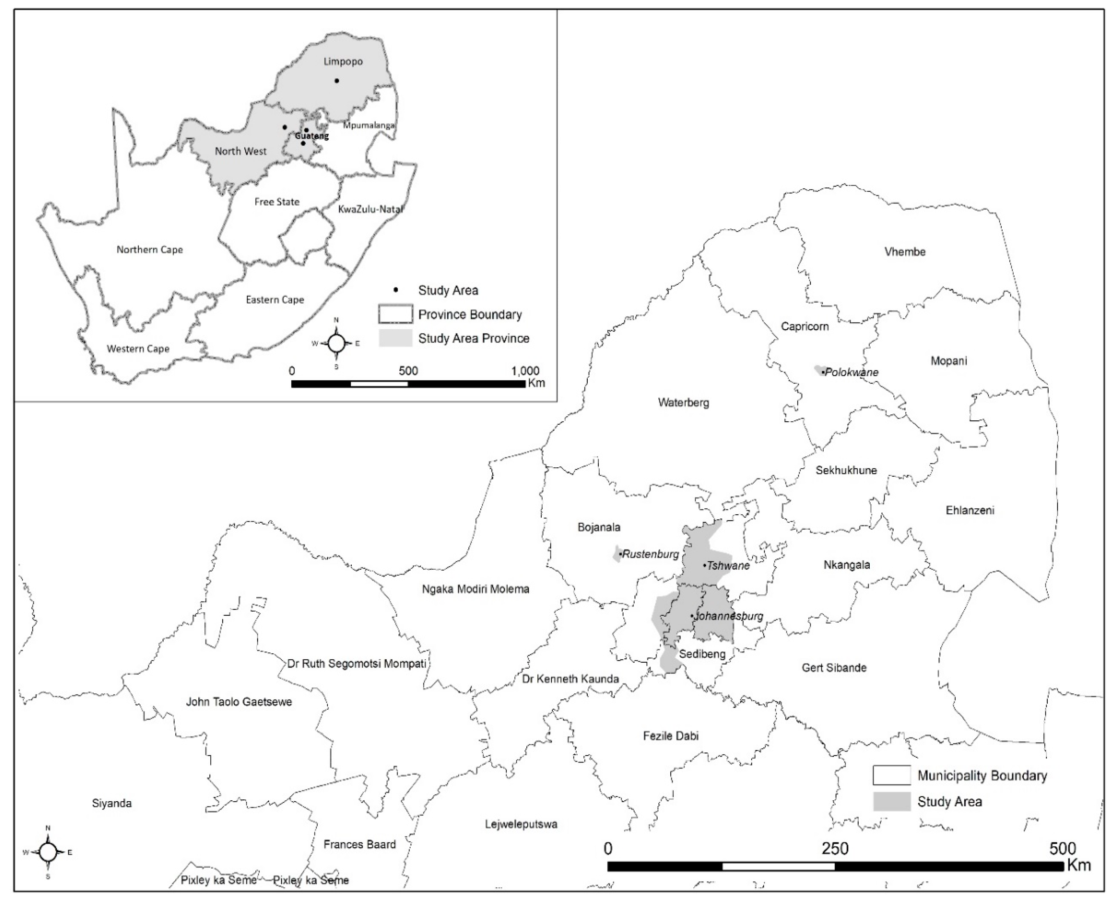
The study area covers Tshwane (also known as Pretoria), Johannesburg, Rustenburg and Polokwane cities in South Africa (see Figure 1 for the geographic location of the study area).

The selection of the four cities was based on their importance in the country. Tshwane and Johannesburg are located in Gauteng province, South Africa’s economic hub and the country’s favourite destination for international and internal immigrants [19]. City of Tshwane lies between the latitudes −25°19′ S and −25°47′ S and the longitudes 27°58′ E and 28°11′ E. It is the administrative capital city of South Africa and is located within the City of Tshwane Metropolitan Municipality (CoTMM). CoTMM has an estimated population of 3,275,152 [20]. Unlike other metropolitan cities in Gauteng province, Tshwane comprises of a significant rural area. The City of Tshwane also consists of a well developed core city and extensive low income and poor communities located in the city periphery. The city’s urban form is influenced by the mountain range which follows the east-west boundary of the metropolitan municipality. The inner city area also comprises many historical monuments and buildings as well as large public spaces [21].

The selected study area of Johannesburg covers the Greater Johannesburg Metropolitan City (GJMC). The GJMC includes the City of Johannesburg and City of Ekurhuleni Metropolitan Municipalities, West Rand and Sedibeng Districts municipalities. GJMC lies between the latitudes −25°47′ S and −26°44′ S and longitudes 27°38′ E and 28°29′ E. The combined estimated population of GJMC is 10.5 million [22]. The city of Johannesburg metropolitan municipality is one of the leading financial centres in the world and is the financial and economic hub of South Africa, contributing more than 16% to the country’s Gross Domestic Product (GDP). As a result, the city of Johannesburg attracts around 3000 migrants every month [23] as people move to the city seeking employment and better living conditions. The city of Ekurhuleni is home to O R Tambo Airport, the biggest and busiest airport in Africa, which facilitates more than 20 million passengers per year [24]. The city contributes 7.7% of South Africa’s GDP, and its economy, whose main sectors include manufacturing, finance and business services is more diverse than that of some of the small countries in Africa [25]. West Rand district municipality is located to the west of the city of Johannesburg and is the poorest region in Gauteng province. Sedibeng district municipality is located in the Southern tip of Gauteng province and is the fourth largest contributor to Gauteng’s economy [26]. Polokwane and Rustenburg are capital cities of Limpopo and North West provinces respectively and are ranked among the fastest growing towns in South Africa. Polokwane lies between latitudes −23°46′ S and −23°56′ S and longitudes 29°18′ E and 29°32′ E, and the local municipality has a population of 628,999 [22]. This figure is expected to increase to almost one million people by 2030 [27]. Owing to its location in the northern part of South Africa, Polokwane has road intersections which connect Zimbabwe and Johannesburg. The city’s attractiveness and rapid growth are associated with its finance and trade sectors [28].

Rustenburg city lies between −25°32′ S and −25°43′ S and longitudes 27°10′ E and 27°18′ E at the foot of Magaliesberg mountain range. The Rustenburg local municipality has a population of 549,600 [22] and is home to the three largest platinum mines in the world [29]. As a consequence, Rustenburg attracts migrants who are seeking work in the mining sector. The mining sector contributes 77% of the city’s Gross Domestic Product (GDP).

3. Data

To map the built-up areas, we used multi-temporal satellite imagery acquired in 1996, 2001–2002 and 2011 by Landsat 5 TM, SPOT 2&5 sensors. Level two Landsat 5 TM images were sourced from United States Geological Survey (USGS) and were downloaded from the Earth Explorer data portal, https://earthexplorer.usgs.gov/. In this study, we used Landsat 5 spectral bands with a 30 m spatial resolution. Level 1A SPOT 2 and Level 3 SPOT 5 images were sourced from the South African National Space Agency (SANSA). The SPOT 2 Panchromatic imagery has a spatial resolution of 10m whereas multispectral imagery has a spatial resolution of 20 m. The SPOT 5 satellite imagery has a spatial resolution of 2.5 m in panchromatic mode and 10 m in multispectral mode.

Table 1. List of the satellite images used for the study and their dates of acquisition.

Study Area	Landsat 5	SPOT 2	SPOT 5
Polokwane	1996/11/30	2002/04/27	2011/07/22
Tshwane	1996/09/11	2001/06/22	2011/07/27
Johannesburg	1996/09/11	2001/07/20	2011/07/27
Rustenburg	1996/08/08	2002/07/18	2011/04/03

. lists the dates of acquisition for satellite images used in different cities.

Population data used in this study was sourced from Statistics South Africa. The population data used was disaggregated to sub-place unit. The sub-place geographic level is the second-lowest level of South African census spatial layers which represent a suburb, village, ward, farm or informal settlement [30]. The population data used for this study was based on censuses conducted in 1996, 2001 and 2011.

4. Method

4.1. Image Classification

Data preparation processes done were orthorectification of the SPOT 2 images and reprojection of all images to Universal Transverse Mercator (UTM) Zone 35S projection system. The SPOT 2 images were orthorectified using the 2011 SPOT 5 images and 20 m Digital Elevation Model. The extraction of SPOT 5 human settlement layer was done using a South African SPOT 5 Global Human Settlement Layer (GHSL) system. The system uses Artificial Intelligence and symbolic machine learning which use radiometric, textural morphological features and reference data to classify built-up areas from non built-up features [31]. Once extracted, the classification results were refined using Erdas Imagine software to reduce the errors of commission in the built-up class.

The extraction of built-up areas from Landsat and SPOT 2 satellite imagery was done using K Nearest Neighbour (kNN) classification technique that uses texture and radiometric values to classify built-up areas from non-built-up areas. Variance Morphological textural features created in Erdas Image Software and Soil Adjusted Vegetation Index (SAVI) were used during classification. The SAVI feature layer was derived using the formula:

$$\frac{\mathrm{N}-\mathrm{R}}{\mathrm{N}+\mathrm{R}+1}\left(L+1\right)$$

where N is the Near Infrared band, R is Red band and L represents the soil adjusted factor [32].

The classification was done using eCognition software. Multiresolution segmentation with a scale parameter of 20, shape value of 0.1 and compactness value of 0.5 was used to generate built-up and non built-up image objects from Landsat and SPOT 2 images. 50 image training samples for built-up areas and 30 training samples for non-built-up areas were created over Tshwane and Johannesburg, whereas 20 built-up and 15 non built-up training samples were created over Polokwane and Rustenburg. Errors of omission and commission were corrected using visual image interpretation.

4.2. Accuracy Assessment

Accuracy assessment of the extracted built-up and non built-up areas was done through visual image interpretation of the classification results against the original images. The accuracy assessment was done using Erdas Imagine software. 100 stratified random points covering both non built-up and built-up classes were created and assessed for Johannesburg and Tshwane. 50 stratified random points were created and assessed for Polokwane and Rustenburg. The points were created randomly within each class across the study area. Producer, Overall and User accuracies were evaluated.

4.3. Change Detection

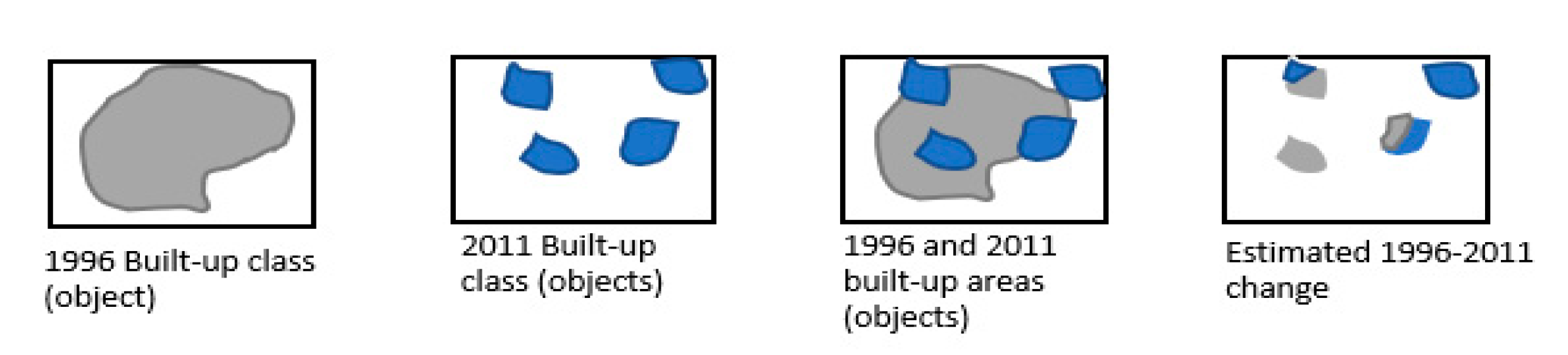
Post-classification change detection technique based on independently classified objects was used to detect urban expansion of the cities from 1996 to 2001 and 2011 in a GIS environment. To assess the built-up area expansion, the equivalent 1996 and 2001 built-up areas were estimated using the 2011 built-up layer. The methodology used for change detection is illustrated in Figure 2.

From Figure 2:

• If blue built-up objects fully intersect with the1996 or 2001 built-up area object (grey), then the resulting built-up represents possible 1996–2001 or 2001–2011 unchanged built-up area.
• If blue built-up objects do not intersect with the 1996 or 2001 built-up area (grey), the built-up area object is considered to be newly built-up areas between 2001–2011.
• The 1996 or 2001 built-up area object that does not intersect with the 2011 built-up areas is considered as non built-up.

This method of assessing built-up area change does not take into account the possible demolition of structures during the period of assessment.

4.4. City Definition Approach

Cities are like living organisms due to their ability to evolve, transform, adapt, innovate and change with emerging trends, such as those originating from local, regional and global forces [33]. In monitoring urban growth rates, the identification of urban/city boundaries should thus be treated with equal dynamism, something that can be achieved by monitoring the changes in a set of unique characteristics. As noted by UN-Habitat, the first principle to achieving accurate and representative estimations for indicator 11.3.1 is viewing urban areas as constantly changing settlements which can expand and/or shrink as a result of various factors, as opposed to viewing them as fixed entities within administratively defined boundaries [34]. Computation of indicator 11.3.1 is thus reliant on accurate identification of the actual areas where urban growth happens over a defined period, which can be achieved through a diversity of spatial analysis approaches [3].

Since the adoption of the SDGs in 2015, global consultations led by UN-Habitat and involving a multiplicity of stakeholders have been held towards the attainment of a globally harmonized city definition approach which can support the computation of indicator 11.3.1 and other indicators which require a clear definition of urban and/or rural areas [3]. Two approaches have been proposed and piloted in different countries across the world: (a) a delineation that uses the concept of urban extent as defined by the character of built-up areas and open spaces [10], and (b) a delineation that uses the degree of urbanization of an area based on both built-up areas and population densities [35,36].

Comparisons undertaken by UN-Habitat and other experts indicate that while the two approaches are conceptually different, their application in large cities produces almost similar boundaries, with more variations reported in smaller towns and urban centres [34]. For this study, we adopted the urban extent approach to city definition [10], which can exclusively be implemented based on analysis of satellite imagery (requires less inputs), and is thus easier to implement than the degree of urbanization which integrates satellite imagery analysis with population data into one-square kilometre grids to identify areas with an urban character.

The urban extent approach to city definition was developed by a team at New York University to facilitate the study of a global sample of 200 cities in the production of the Atlas of Urban Expansion [37], an initiative implemented jointly with UN-Habitat. This approach measures the level of urbanization of an area in four broad steps: (a) extraction of built-up areas/pixels, open spaces and water bodies from satellite imagery, (b) determination of the urban-ness of each built up pixel, (c) association of each open spaces to the surrounding built-up pixel to determine if they are urban or rural, and (d) delineation of the area’s urban extents based on the results from b and c–which represents the urban area boundaries [10].

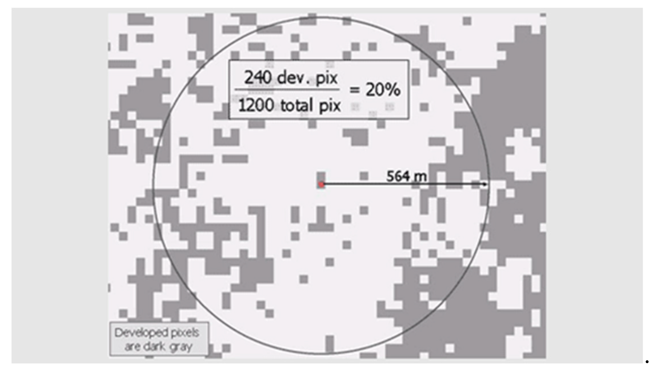
In the first step, satellite images for an area of interest are classified into three broad classes—built-up areas/pixels, open spaces (non-built up pixels) and water. In this approach, built-up pixels are defined as the contiguous areas occupied by buildings and other impervious surfaces. The second step involves computation of neighbourhood statistics against the built-up pixels from the classification. In this step, which is implemented in GIS software, a circle with a radius of 564 meters (an area of one square kilometre) is drawn around each built-up pixel, which constitutes a ten-minute walk [10]. This circle is referred to as the “Walking Distance Circle” to each individual built up pixel (Figure 3). An “If” condition is then applied to each built-up pixel within the walking distance circle to determine whether it is urban, suburban or rural in character, as follows:

• Urban pixels are all the built-up pixels surrounded by a majority (50% or more) of other built-up pixels in their walking distance circle (Figure 3)
• Suburban pixels are all the built-up pixels surrounded by 25–50% of other built-up pixels in their walking distance circle, and
• Rural pixels are all the built-up pixels surrounded by less than 25% of other built-up pixels in their walking distance circle.

In the third step, the open spaces (non built-up areas) in the analysis area are then categorized into one of the following three classes, based on the nature of the surrounding built-up pixels [10];

• Fringe open spaces–consists of all open space pixels within 100 m of urban or suburban pixels;
• Captured open spaces–consists of all open space clusters that are fully surrounded by urban and suburban built-up pixels and the fringe open space pixels around them, and that are less than 200 hectares in area and
• Rural open space–consists of all open spaces that are not fringe or captured open spaces.

In the fourth step, a combination of urban and sub-urban built-up areas and fringe and captured open spaces are used to form a hard edge urban boundary known as the urban extent. In many cases, the resultant urban extent consists of one main urban cluster, surrounded by smaller clusters at varying distances. Where the analysis area is known, local knowledge is used to determine which of the smaller clusters belong to the main cluster (and in turn which smaller clusters get included as part of the urban extent) and/or which smaller clusters form independent settlements. Where this knowledge is non-existent, an inclusion rule based on geographical proximity is applied to achieve similar results [1].

For the delineation of urban extent in this study, a python script was developed in Esri’s ArcGIS software to replicate the methodology developed by Angel et al per the above steps. The input for the script was the built-up layer produced during the image classification stage discussed previously.

4.5. Indicator Computation Approach

In each of the four cities, we analyzed urban change trends over three time periods—1996, 2001 and 2011. For each city, we computed three indicators (a) the ratio of land consumption rate to population growth rate, (b) the land consumption per capita and (c) the percentage change in the built-up area.

The ratio of land consumption rate to population growth rate (LCRPGR) is the core indicator under SDG 11.3.1. It is defined as a ratio of the annual rate at which cities grow spatially to the annual rate of their population growth during a given time period [3]. Ideally, a LCRPGR value less than one means that the annual rate of population growth over the computation period was higher than that of land consumption; a value of one means that the annual rates of population growth and land consumption were equal; while a value higher than one means that the annual rate of land consumption was higher than that of population growth. This simplistic interpretation of the indicator does not however help explain when cities become too congested or when they become too sparsely settled, nor does it adequately account for negative growth [3,8,38]. Owing to these limitations of the LCRPGR measurement, the land consumption per capita and the percentage change in built-up area have been identified as being important explanatory measurements for indicator 11.3.1 [3,38].

The land consumption per capita looks at how much space each person within the city is using at a given time. Some researchers have identified this as a better indicator of measuring land use efficiency than the LCRPGR, particularly because it helps understand intra-city changes [38]. In this study, we computed the land consumption per capita in absolute terms, by dividing the total built-up area within the urban extent at a given year by the population associated to that extent.

The formula adopted for the computation of LCRPGR was based on the UN approved metadata, while the formulas used for the computation of the other two indicators were those recommended by UN-Habitat [37].

Table 2. Indicator computation formulas.

Indicator	Formula	Symbol Explanation
Ratio of Land Consumption Rate to Population Growth Rate (LCRPGR)	$\frac{\mathrm{LN}\left({\mathrm{Urb}}_{\mathrm{t}+\mathrm{n}}/{\mathrm{Urb}}_{\mathrm{t}}\right)}{\left(\mathrm{y}\right)}$/ $\frac{\mathrm{LN}\left({\mathrm{Pop}}_{\mathrm{t}+\mathrm{n}}/{\mathrm{Pop}}_{\mathrm{t}}\right)}{\mathrm{y}}$,	LN-natural algorithm value Urbt-urban extent in km2 for past/initial year Urbt+n-urban extent in km2 for current/final year y-number of years between the two measurement periods Popt-total population within the urban extent in the past/initial year Popt+n-total population within the urban extent in the current/final year.
Land consumption per capita	$\frac{\left({\mathrm{UrBU}}_{\mathrm{t}}\right)}{\left({\mathrm{Pop}}_{\mathrm{t}}\right)}$	UrBUt-total built-up area within the urban extent in time t Popt-total population within the urban extent in time t
Percentage change in the built-up area	$\frac{\left({\mathrm{UrBU}}_{\mathrm{t}+\mathrm{n}-}/{\mathrm{UrBU}}_{\mathrm{t}}\right)}{\left({\mathrm{UrBU}}_{\mathrm{t}}\right)}$ × 100	UrBUt+n-total built-up area within the urban extent for current year UrBUt-total built-up area within the urban extent for past/initial year

summarizes the formulas used for each indicator.

For LCRPGR and the percentage change in built-up area indicators, we analyzed growth over two time periods; 1996 to 2001 and 2001 to 2011; while for the land consumption per capita we computed the indicator for the individual years; 1996, 2001 and 2011.

4.6. Matching Population to Urban Areas

Since the computation of indicator 11.3.1 relies on identification of the actual areas where urban level growth is happening which is not often aligned to existing administrative and/or population boundary units [34], disaggregation of population is a key requirement for the indicator computation. Over the last decade, different initiatives have been implemented in the area of population disaggregation, with most focus put around the creation of population grids. The concepts applied in the creation of population grids range from those which use simple approaches such as areal-weighting or uniform distribution [39,40] to those which integrate ancillary geographical data to implement dasymetric modelling and smart interpolation in order to apportion population to different land use classes [35,41,42,43,44,45]. Key among the global population datasets that apply the different disaggregation approaches include the Gridded Population of the World (GPW), Global Human Settlement Population Grid (GHS-POP) and WorldPop. The underlying concept for these initiatives is the re-distribution of population from the large units in which census data is collected to smaller comparable units or specific locations where people live (such as in buildings or habitable land use classes). These datasets have proven useful for computation of indicator 11.3.1 and other sustainable development goals which require disaggregated population data [8].

In South Africa, population data is released at the sub-place geographic level—the second lowest level of South African census spatial layers which incorporates several enumeration areas [30]. The size of sub-places varies greatly throughout the country, with the smallest unit covering an area of 0.003316 km² and the largest spanning over 3,556,904 km². Based on this, calculating population densities for each sub-place displays huge variations, with high densities often recorded in the smaller sub-places. Where a high density settlement is located within a large sub-place, the population is redistributed to the entire area including un-inhabited parts of the sub-place, significantly distorting the actual densities in the settlement. Some of the current population disaggregation methods seek to correct this problem by assigning populations to only the habitable land use classes e.g., GHS-POP and WorldPop datasets.

In order to match the population data acquired from Statistics South Africa, we implemented the same approach adopted by Angel at al. [10] in the estimation of populations living in each of the urban extents created from satellite imagery analysis. We divided the total population in each sub-place by the total built-up pixels in the same sub-place to achieve a population per pixel value. Here, we made two major assumptions, (a) that every built up pixel is habitable regardless of the land use class it falls in, and (b) since we did not have information on the height of buildings (number of floors), we only considered the built-up areas footprints as opposed to their volumes in the population redistribution. This way, each built up pixel within a sub-place would have the same value – representing the associated population count. The population per pixel values would vary between sub-places, depending on the total population and number of built-up pixels.

To reduce errors of fragmentation associated very small population units such as the built-up pixels [38], we created grid squares measuring 100 by 100 meters over the entire country and overlaid these with the built-up layer containing the population per pixel values for the four cities. We then summed up the population of all pixels within each square grid, to attain a population count per grid cell. Quality assessments were implemented to ensure that the total population for all 100 by 100 grid cells in a given sub-place was always equal to the total population of that sub-place.

To determine the population of the urban extent in a given city and year, we added up all grid cells that intersected with the urban extent using the zonal sum tool in ArcGIS software. We then used the resulting population figure to calculate the population growth rate for each city between the two time periods (1996–2001 and 2001–2011).

5. Results and Discussion

The following sections present the results of the study. Section 5.1 presents the image classification results while Section 5.2, Section 5.3 and Section 5.4 present the urban expansion and population growth trends, the land consumption per capita and the ratio of LCRPGR respectively.

5.1. Image Classification

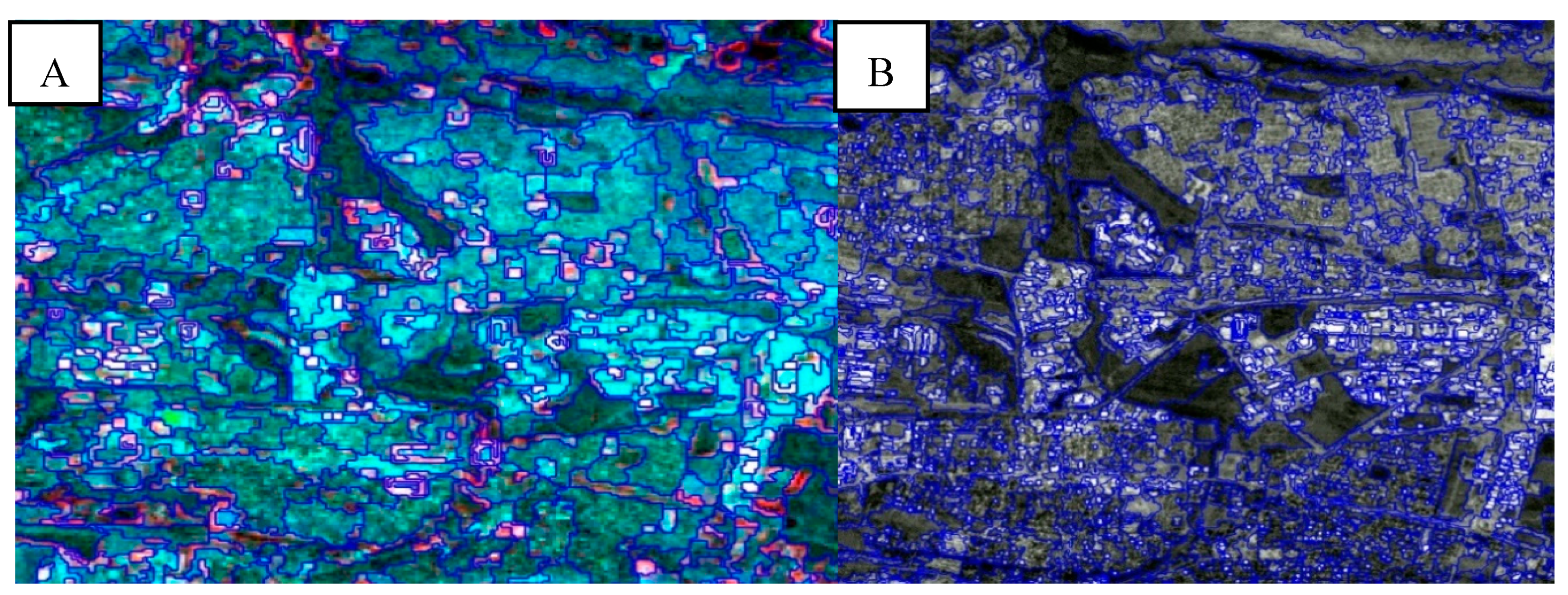
The segmentation results of Landsat 5 and SPOT 2 are shown in Figure 4. The assessment of the segmentation results of Landsat 5 grouped built-up area and smaller open spaces objects within the urban area. Large open spaces which include parks and other non built-up areas were separated from built-up objects using Landsat 5 and SPOT 2 images. The segmentation of SPOT 2 image objects was successful in creating objects that represent more accurate built-up objects and smaller open space objects compared to the segmentation results of Landsat 5.

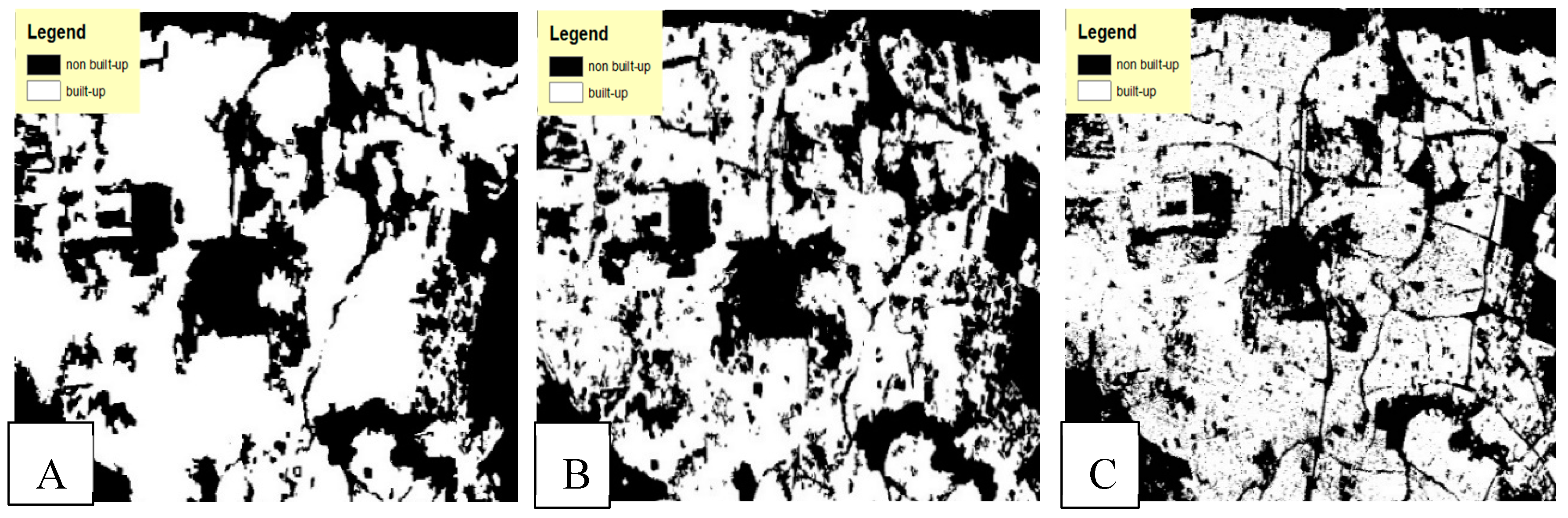
The classification results of built-up and non built-up classes derived from Landsat 5 TM, SPOT 2 and SPOT 5 are shown Figure 5. The South African SPOT 5 GHSL system was successful in distinguishing small open spaces such as sports fields from built-up areas. The kNN object-based classification technique applied to Landsat 5 TM imagery generalized the built-up area and was unable to classify smaller open areas as non-built-up areas. The classification technique applied on SPOT 2 imagery was successful in detecting more open spaces as non built-up areas compared to the results achieved from Landsat imagery.

The accuracy assessment of the classification results shows that the adopted built-up classification methods were successful in distinguishing built-up areas from non-built-up features, with a recorded overall accuracy of 83–93% for all the three years as shown in

Table 3. Accuracy assessment results.

Study Area	1996	2001	2011
Johannesburg
Producer Accuracy (%)	100	84	100
User Accuracy (%)	93	82	80
Overall Accuracy (%)	85	83	90
Tshwane
Producer Accuracy (%)	85	93	90
User Accuracy (%)	89	81	86
Overall Accuracy (%)	84	90	92
Polokwane
Producer Accuracy (%)	83	85	80
User Accuracy (%)	90	93	85
Overall Accuracy (%)	86	88	89
Rustenburg
Producer Accuracy (%)	83	86	80
User Accuracy (%)	100	100	100
Overall Accuracy (%)	93	85	92

.

Even though the accuracy assessment results show high producer, user and overall accuracies, the detection accuracy of 1996 and 2011 built-up areas in small holdings was poor. This may be attributed to the spatial resolution of Landsat 5 and SPOT 2 satellite imagery. This did not affect the computation of the three focus indicators since only urban built-up areas were used.

5.2. Urban Expansion and Population Growth Trends

The classification results show that Johannesburg had the largest built-up areas during the three years of assessment, with 2258.86 km² of built-up areas in 2011, whereas Rustenburg had the smallest built-up areas covering only 75.32 km² in 2011 (

Table 4. Built-up area and population of the built-up areas.

City	Built-up (km2)	Built-up (km2)	Built-up (km2)	Population	Population	Population
	1996	2001	2011	1996	2001	2011
Johannesburg	1571.46	1913.74	2258.86	5,233,186	6,596,987	8,805,405
Tshwane	569.89	731.06	888.54	1,526,161	1,935,484	2,768,399
Polokwane	63.74	76.55	107.43	122,301	169,726	276,703
Rustenburg	42.54	49.81	75.319	122,219	183,982	266,318

).

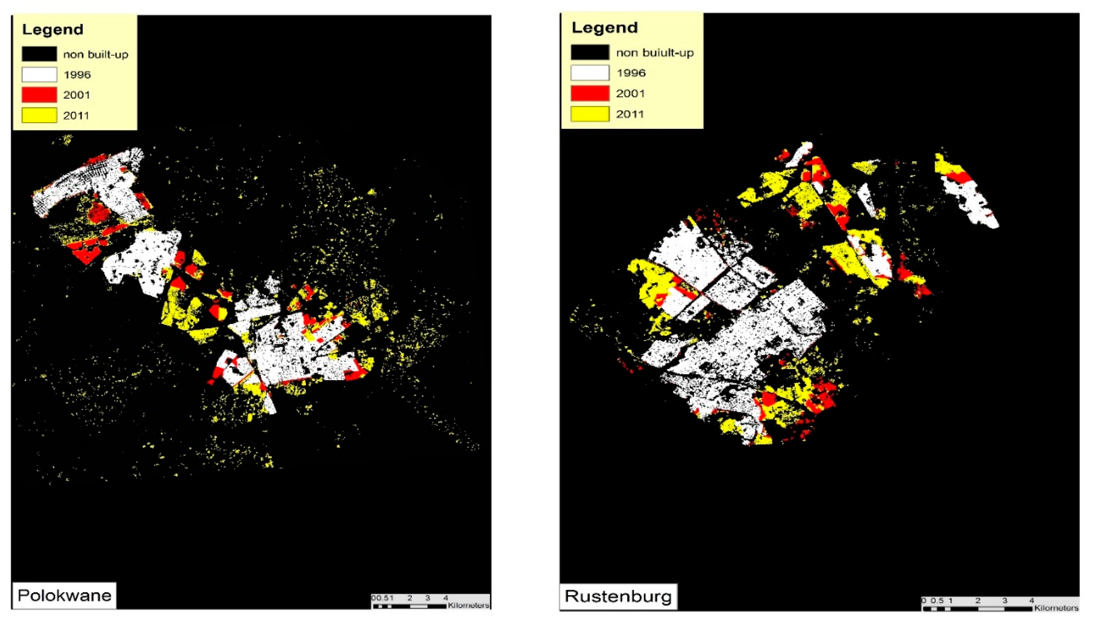
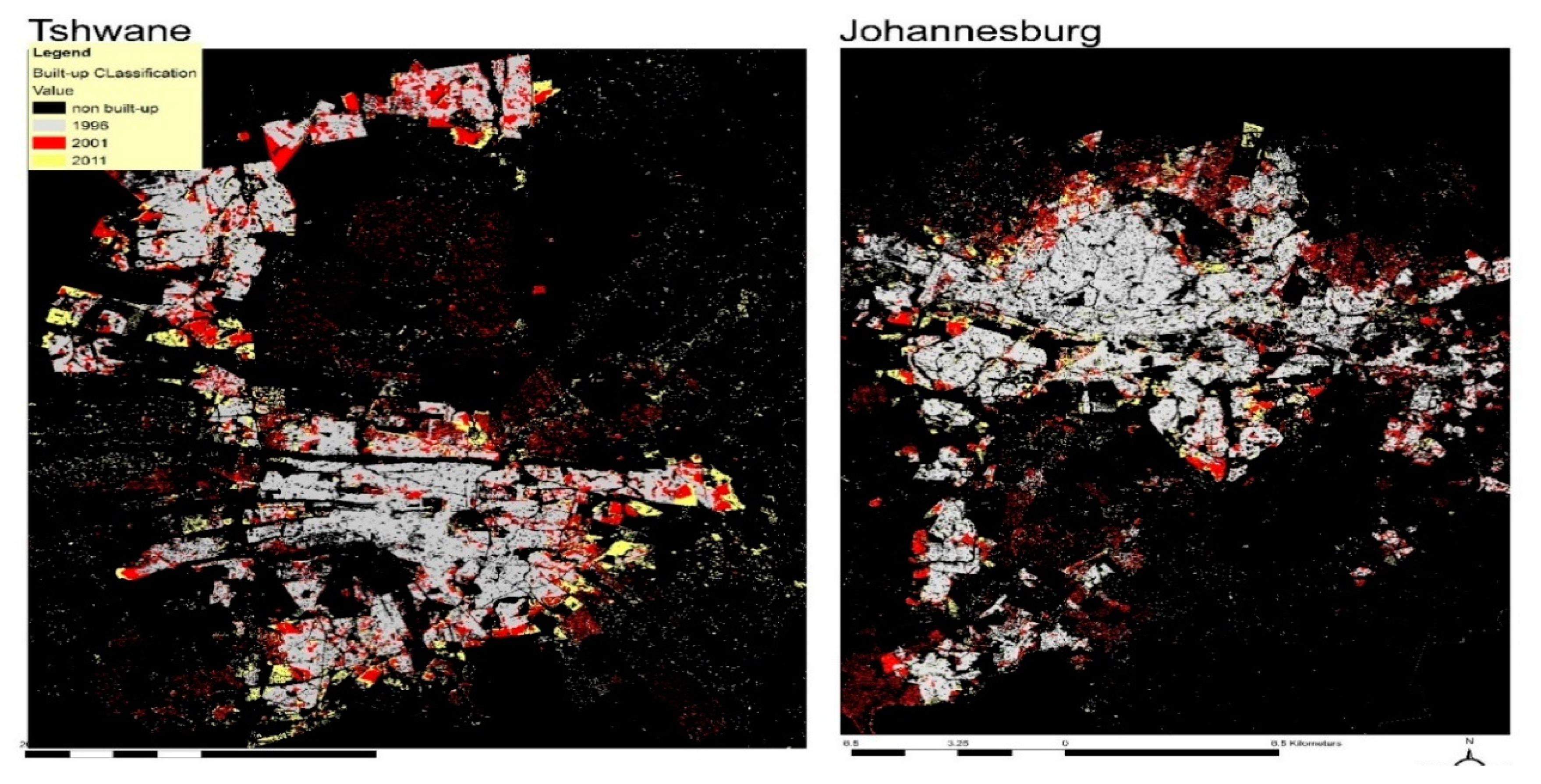
The change detection results for 1996, 2001 and 2011 are shown in Figure 6 and Figure 7.

Table 5. Urban growth or land consumption rate (LCR) and population growth rate.

City	Year	Total Change in Built-up Area * (km2)	Land Consumption Rate (LCR) **	Population Growth Rate (PGR) **
Johannesburg	2001–2011	+345.12	0.017	0.029
Johannesburg	1996–2001	+342.28	0.039	0.046
Tshwane	2001–2011	+157.48	0.020	0.036
Tshwane	1996–2001	+161.17	0.050	0.048
Polokwane	2001–2011	+30.87	0.034	0.051
Polokwane	1996–2001	+12.81	0.037	0.070
Rustenburg	2001–2011	+25.51	0.041	0.067
Rustenburg	1996–2001	+7.27	0.032	0.065

* as per delineated urban extent boundaries; ** LCR and PGR are presented as raw values as opposed to percentages.

summarizes the total change in built-up areas, the Land Consumption Rate (LCR) and Population Growth rate (PGR) over 1996–2001 and 2001–2011 periods. Over the five year period spanning 1996 to 2001, the built-up area in Tshwane increased by 161.2 km², and by 157.5 km² during the ten year period spanning 2001–2011. In Johannesburg, the built-up area increased by 342.3 km² between 1996–2001, and by a further 345.1 km² between 2001–2011. Rustenburg experienced an increase in the built-up area of 7.27 km2 over 1996–2001 period and 25.51 km² over 2001–2011 period, while the built-up area of Polokwane increased by 12.81 km² and 30.87 km² during the same period.

Between 1996 and 2001, Tshwane recorded the highest annual land consumption rate (LCR), computed at 0.05, while Rustenburg recorded the lowest LCR (0.032) during the same period. Over the 2001–1011 period, Johannesburg recorded the lowest LCR, which averaged 0.017 per annum, followed by Tshwane at 0.02. Polokwane and Rustenburg recorded LCR values of 0.034 and 0.041 respectively during the same period (Table 5).

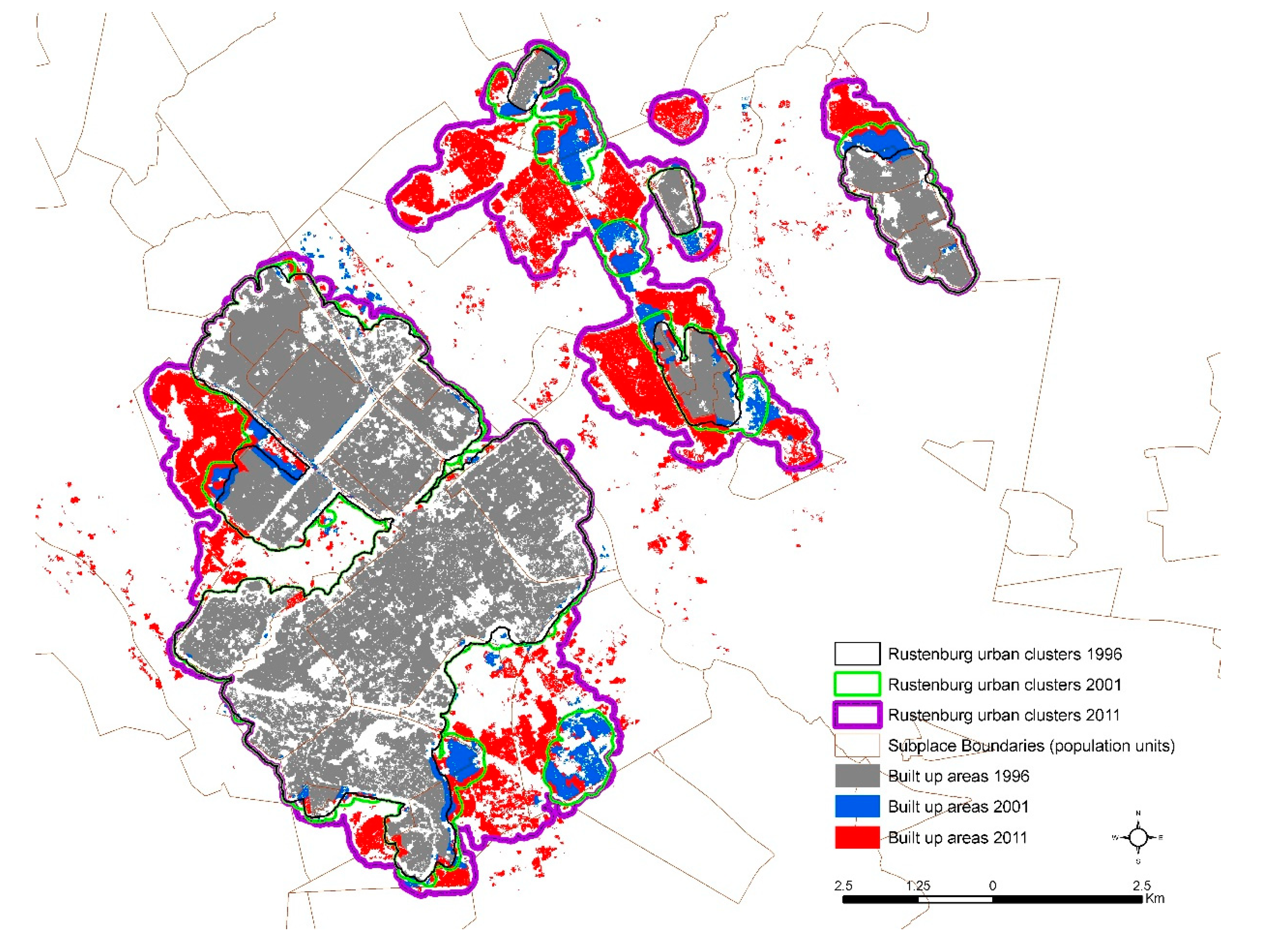
The assessment of the population of the four cities was based on urban extent delineated during the study (refer to Figure 8 for Rustenburg urban extent boundaries for 1996, 2001 and 2011). The results achieved from the matching of built-up areas and population data show that Johannesburg was the most populated city in 2011 with 8,805,404 people, while Rustenburg was the least populated city with 266,318 people (Table 5). The secondary cities witnessed the highest population growth rates from 1999–2001 to 2001–2011 compared to the big cities. Polokwane experienced the highest population growth of 0.070 between 1996 and 2001, while Johannesburg experienced the least population growth rate of 0.046 during the same period. During the 2001–2011 period, Rustenburg experienced the highest population growth rate of 0.067, while Johannesburg experienced the lowest population growth rate of 0.029 during the same period.

To understand densification trends in the four cities, we selected the urban extent boundaries for the median analysis year (2001) and examined how much new built-up areas were added up to 2011. The findings from this analysis were that, Johannesburg experienced the highest densification, with 8% increase in built-up areas within the 2001 boundaries over the 2001–2011 period. This was equivalent to 98.2 km² of newly built-up land. Tshwane and Polokwane followed closely with about 7.4% increase in new built-up areas over the same period, although the absolute increase in newly built-up land varied significantly—from 35.7 km² in Tshwane, to only 3.8 km² in Polokwane. Rustenburg experienced the lowest densification, as recorded through an increase of only 4.4% (1.4 km²) in the total built-up area over the period.

5.3. Land Consumption per Capita

The computation results of land consumption per capita are shown in

Table 6. Computation results of Land consumption rate per capita.

City	Year	Land Consumption per Capita
Johannesburg	2001–2011	164
Johannesburg	1996–2001	198
Tshwane	2001–2011	210
Tshwane	1996–2001	237
Polokwane	2001–2011	252
Polokwane	1996–2001	355
Rustenburg	2001–2011	162
Rustenburg	1996–2001	226

.

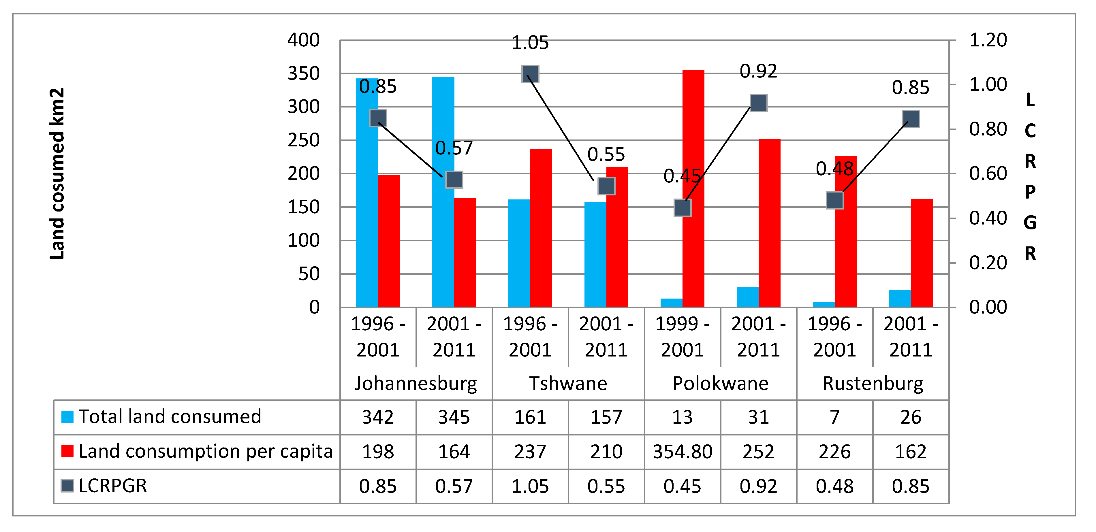
The assessment of the results in Tshwane and Johannesburg shows a decrease in the land consumption per capita, indicating that each person was consuming less built-up space between the 2001–2011 period than the 1996–2001 period. In Johannesburg, the land consumption per capita decreased from198 m² per person in 1996 to 185 m² per person in 2001 and further to 164 m² in 2011. In Tshwane, land consumption per capita increased from 237 m² to 250 m² over the 1996–2001 period. This value dropped to 210 m² over the 2001–2011 period. The decrease in land consumption per capita in these cities indicates densifying settlements and is consistent with the observed total change in built up areas. On the other hand, Polokwane and Rustenburg recorded an overall reduction in land consumption per capita, indicating that the secondary cities were also densifying, albeit at a slower pace than the major cities.

5.4. Ratio of Land Consumption Rate to Population Growth Rate

The computation results of the Ratio of LCRPGR are shown in

Table 7. Computation results of Ratio of Land Consumption Rate to Population Growth Rate (LCRPGR).

City	Year	Ratio of Land Consumption Rate to Population Growth Rate (LCRPGR)
Johannesburg	2001–2011	0.57
Johannesburg	1996–2001	0.85
Tshwane	2001–2011	0.55
Tshwane	1996–2001	1.05
Polokwane	2001–2011	0.92
Polokwane	1996–2001	0.45
Rustenburg	2001–2011	0.85
Rustenburg	1996–2001	0.48

.

Johannesburg recorded a decline in the ratio of LCRPGR, from 0.85 during the period 1996–2001 to 0.57 during the period 2001–2011. A similar trend was observed in Tshwane, whose ratio almost halved from 1.05 in the 1996–2001 period to 0.55 between 2001 and 2011. The LCRPGR ratios for Polokwane and Rustenburg were 0.45 and 0.48 during the period 1996–2001, which increased to 0.92 and 0.85 respectively during the 2001–2011 period. The general implication of this growth trend is that, during the 1996–2001 period, the two major cities experienced a relatively faster rate of urban sprawl than the secondary cities, which was reversed during the 2001–2011 period. These findings are corroborated by the rates of land consumption as shown in Table 5 as well as the total increase in built-up area and land consumption per capita. Figure 9 summarizes the observed growth trends for the three computed indicators.

The higher ratio of LCRPGR in Johannesburg and Tshwane between 1996 and 2001 may be attributed to the abolishment of the apartheid laws in the early 1990s which resulted in increased migration of mostly black people from rural areas and neighbouring countries to the cities in search of employment and better living conditions. This trend was not observed in smaller cities since they did not offer a lot of opportunities to attract many immigrants at that time. The decline of the LCRPGR ratio in Johannesburg and Tshwane between 2001 and 2011 may have been influenced by targeted efforts by the government of South Africa and the relevant municipal authorities to promote the development of sustainable human settlements. For example, “Breaking New Ground”: A Comprehensive Plan for Human Development of Sustainable Human Settlements was enacted in 2004 to not only fast-track service delivery but also to ensure sustainable development of human settlements.

The increase in LCRPGR ratio in Polokwane and Rustenburg over the 2001–2011 period could partly be influenced by the government led informal settlements upgrading programme (ISUP) which builds adequate housing structures for people living in informal settlements, majority of which are greenfield projects. The increase in housing developments in Rustenburg could also be attributed to mixed housing projects by the state and mining companies operating in the area who seek to provide housing for their mining staff. In addition to a growing economy which is associated with centralisation of provincial government departments and other services such as public broadcasting, development of government-financed low-cost housing projects could be contributing to higher urban expansion rates of Polokwane.

6. Conclusions

The study assessed the SDG indicator 11.3.1 and urban growth patterns in two major and two secondary cities using built-up areas mapped from medium and high spatial resolution satellite imagery extracted using different classification methodologies. The adopted change detection methodology allows for the visualization of possible built-up expansion or densification of cities and available non-built-up areas at a higher spatial resolution compared to spatial resolution of historical images. Even though the method does not take into account possible demolition of the built-up structures, the visualization of historical built-up expansion results at high resolution may encourage authorities to use the information of urban growth and the data layers during planning. The computation of land consumption per capita and total change in built-up area together with SDG Indicator 11.3.1 provides essential information that can be used to understand better urban growth patterns of cities. Further, this study has shown the relevance of adopting a city definition approach that is not fixed to the administrative boundaries for measuring indicator 11.3.1 and understanding the full extent of urbanization trends in cities, which is crucial in the formulation workable strategies aimed at making cities and human settlements resilient, inclusive, safe and sustainable. Finally, the study confirmed the common narrative that small and secondary cities in Africa are growing at a faster rate than the big cities, not only in terms of population growth rate but also in terms of spatial expansion.