Article

Impact of Indo-Pacific Climate Variability on Rice Productivity in Bihar, India

1
Department of Geography, Delhi School of Economics, University of Delhi, Delhi 110007, India
2
Disaster Prevention Research Institute, Innovative Disaster Prevention Technology and Policy Research Laboratory, Kyoto University, Gokasho, Uji City, Kyoto 611-0011, Japan
3
Application Laboratory, Japan Agency for Marine-Earth Science and Technology, Kanagawa 2360001, Japan
4
Department of Environment Science, Fakir Mohan University, Odisha 756020, India
5
State Key Laboratory of Desert & Oasis Ecology, Xinjiang Institute of Ecology & Geography, Chinese Academy of Sciences, Urumqi 830010, China
6
Faculty of Environmental Earth Science, Hokkaido University, Sapporo 060-0810, Japan
7
Graduate School of Advanced Integrated Studies (GSAIS) in Human Survivability (Shishu-Kan), Kyoto University, Kyoto 606-8501, Japan
*
Author to whom correspondence should be addressed.
Sustainability 2020, 12(17), 7023; https://doi.org/10.3390/su12177023
Submission received: 9 July 2020 / Revised: 24 August 2020 / Accepted: 26 August 2020 / Published: 28 August 2020

Abstract

:
The impact of Indo-Pacific climate variability in the South Asian region is very pronounced and their impact on agriculture is very important for the Indian subcontinent. In this study, rice productivity, climatic factors (Rainfall, Temperature and Soil Moisture) and associated major Indo-Pacific climate indices in Bihar were investigated. Bihar is one of the major rice-producing states of India and the role of climate variability and prevailing climate indices in six events (between 1991–2014) with severer than −10% rice productivity are analyzed. The Five-year moving average, Pearson’s Product Moment Correlation, Partial Correlation, Linear Regression Model, Mann Kendall Test, Sen’s Slope and some other important statistical techniques were used to understand the association between climatic variables and rice productivity. Pearson’s Product Moment Correlation provided an overview of the significant correlation between climate indices and rice productivity. Whereas, Partial Correlation provided the most refined results on it and among all the climate indices, Niño 3, Ocean Niño Index and Southern Oscillation Index are found highly associated with years having severer than −10% decline in rice productivity. Rainfall, temperature and soil moisture anomalies are analyzed to observe the importance of climate factors in rice productivity. Along with the lack of rainfall, lack of soil moisture and persistent above normal temperature (especially maximum temperature) are found to be the important factors in cases of severe loss in rice productivity. Observation of the dynamics of ocean-atmosphere coupling through the composite map shows the Pacific warming signals during the event years. The analysis revealed a negative (positive) correlation of rice productivity with the Niño 3 and Ocean Niño Index (Southern Oscillation Index).

1. Introduction

The Indo-Pacific Ocean basin plays a very important role in deciding the amount of rainfall observed and it directly influences the crop production in the South Asian region [1,2]. Along with rainfall, the impact of variation in temperature is also very high with rice production and discussed in the case of the South Asia region by Abbas and Mayo (2020) [3]. An important teleconnection detection based study to find the impact of corn yield in the USA revealed a high association with the Arctic Oscillation [4]. Moreover, the high association with the Monsoon Index in spite of El Niño-Southern Oscillation (hereafter ENSO) based indices was found while analyzing the teleconnection of various climate indices with the rice and maize yield for the Indian case [5]. Local factors play a major role in the quantity of rainfall and productivity depends on it. In a perception-based study, the role of many local factors was highlighted and the role of heavy/low rainfall leading to the declining crop productivity was discussed [6,7].
Sometimes, one climate index influences the intensity of another and thereby changing the potential response to a teleconnection region [8,9]. Local factors play a major role in regulating the local climate also and therefore production is affected by it [10,11]. A lot of studies related to different parts of the globe discussed the relation of climate indices with crop production and some very important studies were on in the South Asian region. Teleconnection impact of ENSO, Indian Ocean Dipole (hereafter IOD), Tropical Atlantic Variability and North Atlantic Oscillation on wheat, maize and soybean was calculated on a global scale and found the substantial impact of ENSO based episodes in the majority of cases across the globe [12,13,14]. Ubilava and Abdolrahimi (2019) worked on maize yield and its teleconnection with ENSO. They found the decline in yield by more than 20% during El Niño like events and explained the high vulnerability [15]. On the other hand, Roberts et al. (2008) found a similar inverse trend between El Niño events and rice production in the Philippines and found the impact to be high there due to rainfed agriculture [16].
The sea surface temperature (hereafter SST) of the tropical Indian and the Pacific Ocean influences rainfall patterns over the globe [8,17,18]. Considering SST as a highly important factor, an assessment of climate impact was carried in the present study with Oceanic Niño Index (hereafter ONI), Niño 3, Southern Oscillation Index (hereafter SOI), El Niño Modoki Index (hereafter EMI), Dipole mode index (hereafter DMI), Trans Niño Index (hereafter TNI), and Monsoon Index (hereafter MI). ONI, Niño 3, SOI, EMI, TNI represents different regions within the tropical Pacific Ocean [8,19,20,21,22], whereas DMI and MI are from the Indian Ocean region. For clarity, the spatial domains represented by these indices are documented in Section 2.3. Oscillation in the oceanic temperature is generally associated with the local atmospheric convection and warming (cooling) of the overlying atmospheric layer, which in turn remotely affect the atmospheric conditions of distant places through teleconnection [23,24]. Impacts of ENSO events and DMI for the Indian subcontinent are known in detail. However, investigation of the contribution of the intensity of a particular index is of high interest to lessen the negative repercussion to different sectors of the economy [25,26].
Rice is a staple crop for most of the northern states in India and a source of food with a high carbohydrate level. Any decline in the total production of rice leads to a negative impact on food security and the sustainable livelihood of farmers. Therefore, as far as the teleconnection part is concerned, the dynamics of the ocean-atmosphere have a lot of societal ramifications and to know the relation of a particular climate index impacting some regions is very important [27]. In some of the previous studies, attempts were made to assess the impact of climate on rice production [28,29,30] as well as projecting the rice production using seasonal climate forecasts [31].
The ideal range of rainfall required for the production of rice varies between 1100 and 1250 mm whereas the temperature requirement varies with the growth stage of rice during the whole growing period [32,33]. On average, the range of surface air temperature required for rice during different stages of growth varies from 21 to 37 °C and at the time of ripening the ideal range of temperature should be between 20 and 25 °C [34]. The water requirement of rice crop remains at its peak between the active tillering and flowering stage and it makes 70% of the total water requirement [33]. Active tillering to the flowering stage is the phase of 30 days to 75 days after germination [35].
Consequences of ENSO impacts on India are well known yet different regions within India get varying responses. While highlighting the fact of rice being the staple crop in the Ganges-Brahmaputra basin, Asada and Matsumoto (2009) elaborated on the high impact of drought (flood) in the upper Ganges (lower Ganges) basin [36]. Knowing the magnitude of impact on rice productivity in Bihar and the huge population depending on it for sustainable livelihood, it was essential to find the teleconnection of rainfall and temperature conditions with different climate indices in relation to rice productivity in Bihar.
The present study discusses the productivity of rice in Bihar (major rice-producing state of India) in relation to the role of different climate drivers influencing rice productivity. The teleconnection of different climate indices was examined using Pearson’s Product Moment Correlation (hereafter PPMC) and results were enriched through Partial Correlation. The possible impact of climate variability was looked into by taking climate indices independently and mutually. The Linear Regression Model, Mann Kendall Test, Sen’s Slope and statistical techniques were also used to discuss the periodic trend of climatic variables and their association with rice productivity [37].
We obtained highly important results signaling the strong association of different climate indices in different seasons. ONI, Niño 3 and SOI showed a very strong connection for different seasonal correlation values with the productivity in Bihar. The present study is of high relevance to the policymakers and the stakeholders, in which the sustainable livelihood is directly linked to rice productivity.

2. Materials and Methods

2.1. Study Area

The Indian state Bihar is located in the Indo-Gangetic plain (Figure 1) and has a total of 3.6 million-hectare area under rice cultivation in 2015-16 [38]. The state has a large population, i.e., 104 million according to the 2011 census [39]. Out of the total population, 92 million live in rural areas in the state, which accounts for 88.71% of the total population [40]. Climate variation plays a big role in rice productivity and directly harms the sustainable livelihood of this rural population like other populous regions of the world [41,42,43,44]. The majority of rice production in Bihar is under rainfed conditions [45]. Variation of rainfall in Bihar plays a very important role in determining the productivity of rice and it is vulnerable to the failure of monsoonal rainfall received in the July-August-September (hereafter JAS) season.
Anomalies of rainfall, temperature and soil moisture in Bihar were analyzed for the period, i.e., one month after the germination of the rice crop. In Bihar, rice is produced in three different seasons, i.e., Kharif (Sowing: June to August, Harvesting: September to November), Rabi (Sowing: October to November, Harvest: April to May) [40] and Summer (Sowing: January to February, Harvest: May to mid-June, only in the irrigated areas) [34]. Each season has its share of importance in the total rice production [46,47,48], though in the case of Bihar, the Kharif season consistently remains to be the main season of rice production.
On average, the Kharif season accounts for more than 93% of annual production during 1997–2014 (Open Government Data Platform India, https://data.gov.in/catalog/district-wise-season-wise-crop-production-statistics). Therefore, the JAS season’s climate is the most important player in productivity after one month of sowing of Kharif crop in June. Hence, the event years were enlisted based on the season whenever the decline in rice productivity of the Kharif season was severer than −10%. Moreover, we considered different seasons of climate indices in relation to the rainfall season (JAS) to look into the influence based on the changing conditions in the preceding season of the rainfall season.
The other seasons were further investigated through the analysis of soil moisture, after one month of sowing in all the three rice growing seasons, i.e., Kharif, Rabi, and Summer. It was noted that the productivity of rice remained good in the ENSO neutral years, with the exception of some years with the influence of local factors on production. On the other hand, the variability or a shift in ENSO events may bring more harmful results to rice productivity in the Bihar [49].

2.2. District Wise Rice Productivity

District-wise data on rice productivity was taken from the Handbook of Statistics [38,50,51,52,53]. The effect of agricultural input and mechanization were normalized in this study by making a five-year running mean for rice productivity. It helped us to find out the climate relationship with rice productivity through some of the important climate indices. Here the impact of climate variability was investigated therefore the absolute impact (gradual and long term) induced due to climate change and non-climatic factors were not analyzed [54].
The year to year rice yield variation ( A ) was defined as the anomalous percentage deviated from the five-year running mean, A = A A ¯ A ¯ × 100 , where A was the annual rice yield and A ¯ was the five-year running mean with the interval of t− 2 to t + 2. Here, initialization of the five year moving average calculation was done with 1989–1990. t was the first year of the whole period, i.e., 1991–1992 and t + 2 (t − 2) was 1992–1993 and 1993–1994 (1989–1990 and 1990–1991). A choropleth map was drawn to show district wise spatial distribution of rice in Bihar (Figure 1). In this study, we used the average of normal years (years other than event years) as the base period for calculation of the climate variable’s anomaly in event years.

2.3. Climate Variables/Indices and SST Data

Rainfall (0.25° × 0.25°) [55] and Temperature (1° × 1°) [56] grid data for 1990–2015 were obtained from the National Climate Centre, India Meteorological Department, Government of India. Climate Prediction Centre soil moisture (V2) data (0.5° × 0.5°) [57] and Global daily SST data (0.25° × 0.25°) [58] were provided by NOAA/OAR/ESRL PSD, Boulder, Colorado, U.S.A. NOAA/NCEP/ NCAR/CDAS-1 daily zonal wind (850 hPa) [59] data set of 2.5° × 2.5° resolution and OLR from NOAA/NCEP/CPC/GLOBAL daily data [60] of 2.5° × 2.5° from January 1990 to December 2015 were used for composite index along with SST. We used the finest possible resolution of data for all the variables used for Bihar and the grid data in the present study was used to observe the spatial pattern of the variables in the different time periods and how they behave in relation to the climate indices. While analyzing the trend and finding the association of climatic variables with productivity, field means of the grid data for Bihar were calculated. Interpolation techniques were used to standardize the resolution.
Rainfall anomaly was plotted over the district map of Bihar for the JAS season only. November-December-January (hereafter NDJ) and March-April-May (hereafter MAM) were selected to look into the availability of soil moisture. Negligible rainfall in both the seasons (NDJ and MAM) was the requirement to consider soil moisture anomaly data. In general, the decline in the JAS seasonal rainfall used to have a prolonged impact on the irrigation of rice drop due to lack of available surface water [61].
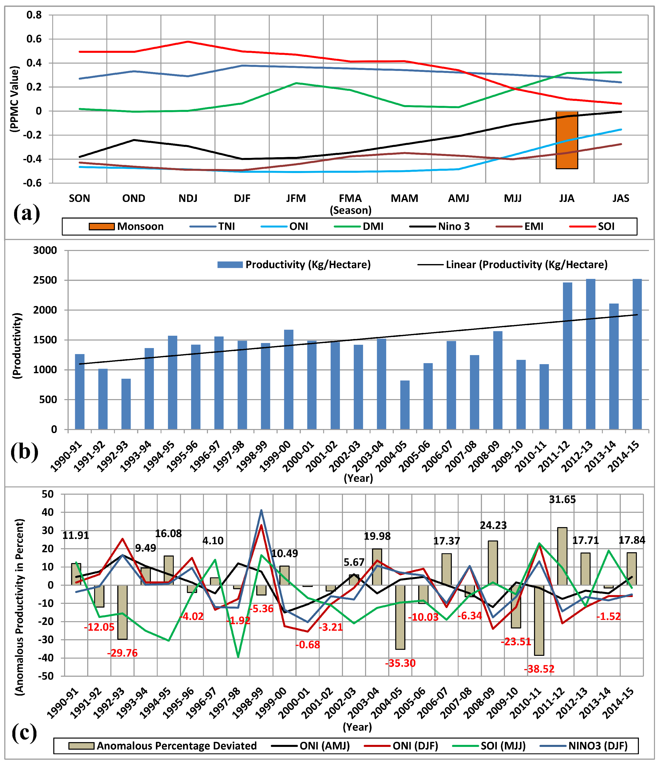
MI was derived from the difference of mean zonal wind between Southern (40° E–80° E, 5° N–15° N) and Northern (70° E–90° E, 20° N–30° N) [20]. ONI was obtained from CPC, NOAA and it was the measurement of running three months SST in Niño 3.4 region (5° N–5° S, 120° W–170° W). TNI was defined as T N I = S S T 1 + 2 N i n ˜ o S S T 4 N i n ˜ o . In this equation SST means normalized SST, 1 + 2 region means Niño 1 + 2 region, and 4 N i n ˜ o means Niño 4 region [62]. DMI is the indicator of IOD, and IOD plays an important role in influencing the summer monsoon rainfall in India [63,64]. Along with the independent impact of IOD, the mutual impact of IOD with ENSO events is also of great value, therefore IOD index was also used in this study [65]. The difference between the SST anomaly of the region lying within 50° E–70° E, 10° S–10° N and 90° E–110° E, 10° S is known as DMI [66]. DMI monthly data in this study were obtained from the online portal of the Japan Agency for Marine-Earth Science and Technology (hereafter JAMSTEC) [67]. Along with ONI, Niño 3 was considered in this study, which is represented by the SST anomaly in the region (5° N–5° S, 150° W–90° W). When it crosses the threshold of 0.5 °C, it impacts Indian summer monsoonal rainfall [68,69]. EMI is also considered an important indicator of climate variability in India [21]. Monthly EMI values were taken from JAMSTEC’s online facility. Data of SOI was acquired from the Climate and Global Dynamics Laboratory (CGD) of the National Center for Atmospheric Research (hereafter NCAR). SOI is calculated by subtracting the monthly sea level pressure anomalies of Tahiti from Darwin [19]. We used all these important indices to investigate the seasonal correlation through PPMC with rice productivity as a part of the initial step (Figure 2a). The linear trend of productivity anomaly as shown in Figure 2b convinced us to look into the annual correlation with the indices having a good correlation shown in Figure 2c.
Along with all the climatic variables, temperature, being one of the highly important ones, also plays an important role in deciding total productivity of crop [70], therefore to look into the role played by temperature, all the events with severer than −10% decline were considered. Temperature anomaly composite of JAS, NDJ and MAM season for all declining years were represented through choropleth (color fill) map using all the variants of temperature, i.e., maximum, minimum and mean and seasonal maps for the particular decline, showed the prevailing maximum and minimum temperature (Figures S1 and S2).

2.4. Methods

PPMC is used to examine the linear association between the yearly rice productivity and climate indices of different seasons [71]. It reveals the one to one association of seasonal indices with the productivity of rice. The correlation for all the years from 1991–2014 was calculated to find the general trend of relationship (Figure 2a) and later on, Particular PPMC, the General Partial Correlation and Particular Partial correlation were calculated (in this article Partial Correlation dealt with rice productivity and two climate indices, here one climate index was made silent as per the procedure of Partial Correlation calculation). Particular PPMC and Partial Correlation dealt with the event years only. PPMC is widely used statistical techniques and is expressed here in Equation (1).
r = n ( x y ) ( x ) ( y ) [ n x 2 ( x ) 2 ] [ n y 2 ( x ) 2 ]
Here x is the independent variable, whereas y is the dependent variable represented by the rice productivity in this study.
Now, we calculated the Particular PPMC to observe the one to one association of major climate indices with rice productivity. Hereafter, filtration was adopted to find the larger side of impact on rice productivity by General Partial Correlation value. The General Partial Correlation here means the whole time period considered in the present study irrespective of the event years (the year with severer than −10% decline). This produced a much clearer picture of the correlation while controlling the effect of other indices. It directed us to some particular seasons for calculating the Particular Partial Correlation. Calculation of the Particular Partial Correlation here means the calculation of Partial Correlation for the event years only, hence this was the last level of filtration adopted in the study. The formula used to calculate the Partial Correlation is mentioned here in Equation (2) and here correlation is calculated for A and B while taking away the effect of C.
r ABC = r AB r AC r BC ( 1 r AC 2 ) ( 1 r BC 2 )
The Partial Correlation was calculated in general for the period 1991–2014 and in particular for the event years and Particular Partial Correlation was calculated for all the seasons, i.e., August-September-October (hereafter ASO), September-October-November (hereafter SON), October-November-December (hereafter OND), NDJ, December-January-February (hereafter DJF), January-February-March (hereafter JFM), February-March-April (hereafter FMA), MAM, April-May-June (hereafter AMJ), May-June-July (hereafter MJJ), June-July-August (hereafter JJA) and JAS and compared with the significant high value of General Partial Correlation. The significance of the correlation results was based on 90% level of significance using one-tailed Student’s t-test. Along with the PPMC and Partial Correlation, we used the Linear Regression Model to quantify the impact of the climatic condition on rice productivity. Mann Kendall Test along with Sen’s Slope was also used to look into the existence of monotonous trend and magnitude of the monotonous trend [72,73,74]. Linear Regression is generally used to look into the relationship between two variables and the value of slope (b), intercept (a) and p-value (significance level) make it easy to understand the one to one relationship. The value of b here assists to understand the potential impact on rice productivity due to change in the climatic variable (i.e., temperature or rainfall).
y = a + b x

3. Results

In order to understand the regional variations in the ENSO impacts on Bihar, the investigation was done on the basis of productivity for the period 1991–1992 to 2014–2015. Districts with high productivity (>2000 kg/ha) are Rohtas, Buxar, Bhabua (Kaimur), Lakhisarai, Arwal, Aurangabad, Bhojpur and West Champaran, and districts with moderate productivity (1500–2000 kg/ha) are Purba Champaran (West Champaran), Patna, Jehanabad, Gaya, Sheikhpura, Nawada, Banka and Katihar (Figure 1). An upward trend was noted in rice productivity (Figure 2b) though the fluctuations prevail over the years. Productivity was found to be negatively (positively) correlated with the ONI, and Niño 3 (SOI) (Figure 2a). Results of PPMC for SOI (ASO-AMJ), TNI (NDJ-MAM), ONI (ASO-MJJ), Niño 3 (ASO to JFM) and MI (JJA) are significantly different from 0 with 90% level of significance. Whereas the increase in the maximum surface temperature in Bihar negatively impacted the rice productivity, and rainfall had a positive relation. Some exceptional local events sometimes played their role in dissipating teleconnection impacts associated with climate indices. These major findings are discussed in detail in Section 3.

3.1. Climate Variability and Rice Productivity

The role of different climate phenomena was investigated by calculating PPMC of rice productivity with different climate indices, i.e., ONI, Niño 3, SOI, EMI, DMI, TNI, and MI. Among all the indices, SOI showed the highest PPMC (1991–2014) running through SON to DJF (Figure 2a). Among all the seasons, DJF showed comparatively high value (significant at 90% level) of PPMC −0.5043, 0.4964, −0.4930, −0.3910 and 0.3781 for ONI, SOI, EMI, Niño 3 and TNI respectively (Table S1). We calculated PPMC for the event year following these observations. When event years were taken together, the high PPMC value was obtained for DMI (0.758) in AMJ, EMI (−0.746) in JJA, MI (−0.627) in JAS, Niño 3 (−0.555) in JFM, SOI (0.546) in NDJ and ONI (−0.526) in AMJ seasons respectively (Table S2). High correlation value does not mean that it is significantly different from zero.
Hence, DMI could not be considered further due to non-significant correlation value and TNI got eliminated with a weak strength of the correlation. As a part of the subsequent step to separate the impact of one index from the other, we calculated the Partial Correlation with EMI, MI, Niño 3, SOI and ONI for the whole period, i.e., 1991–1992 to 2014–2015. Calculation of Partial Correlation presented a clear picture that DMI, MI, TNI and EMI do not play a major role in independent mode (Table S3). Whereas, removing their influence on Niño 3, ONI and SOI emerged effectively. Therefore moving on to the next step of refining our results on climate indices and their relation with rice productivity, we adopted the Particular Partial Correlation. Particular Partial Correlation dealt with the six identified event years only. In a nutshell, results of this particular correlation revealed the major climatic indices with the utmost impact on rice productivity.
Results of Particular Partial Correlation (Table S4) reflect in ONI’s case that removing the influence of TNI (ASO, SON, OND and NDJ season) yields significant very high correlation values. DMI’s influence in OND and NDJ season for almost the whole years yielded a good correlation. In addition to it, the case of removing the EMI’s influence of almost all its seasons proved effective in a strong correlation of ONI. In the case of Niño 3, it remained dominant from DJF to FMA when the influence of TNI in its ASO to NDJ seasons, DMI in its SON to NDJ season and EMI in its ASO to NDJ and JJA to JAS season were removed. Whereas, SOI was found dominant mainly in JJA when the role of TNI for SON to AMJ, DMI for ASO to NDJ and EMI for SON to DJF were removed. Climatic phases with significant correlation and value with >0.5 and <−0.5 are tabulated in Table 1 and this table shows the most refined results for rice productivity and its association with climate indices.

3.2. Rainfall and Soil Moisture

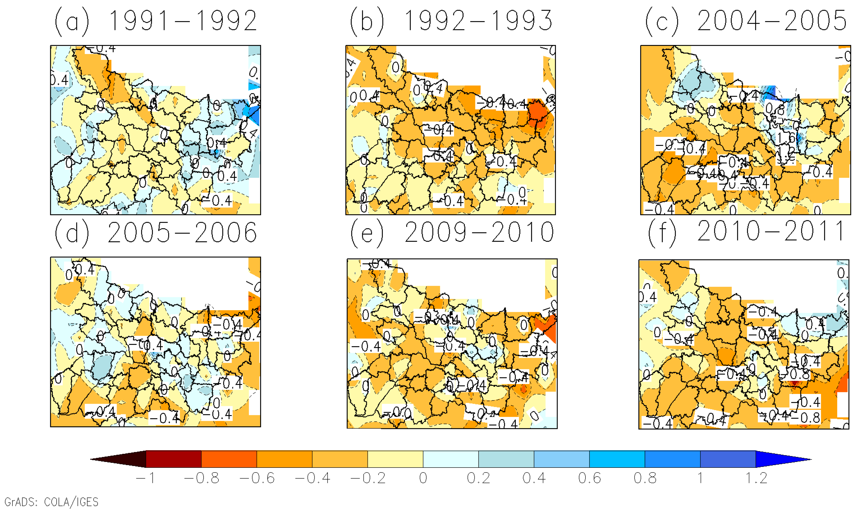
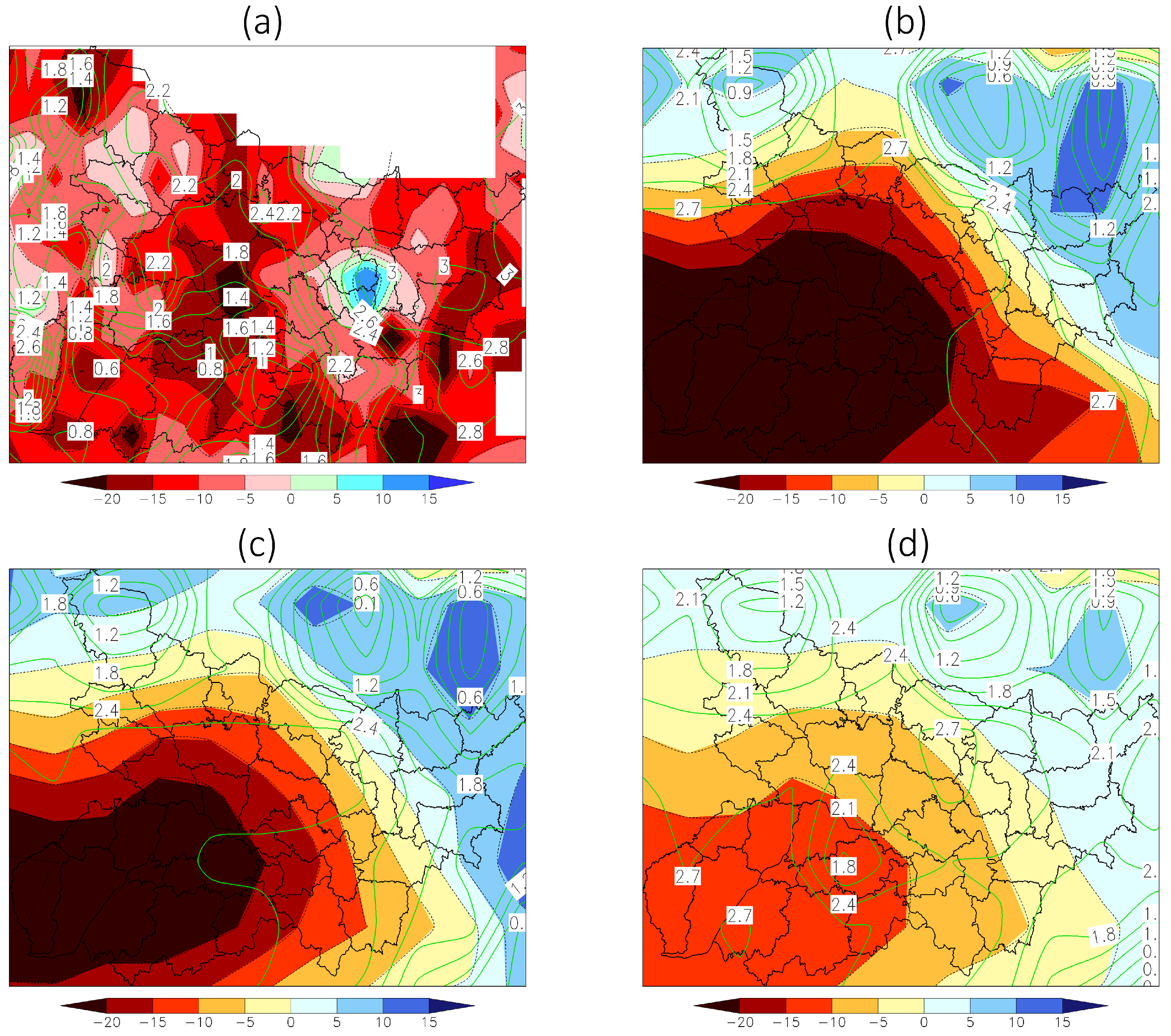
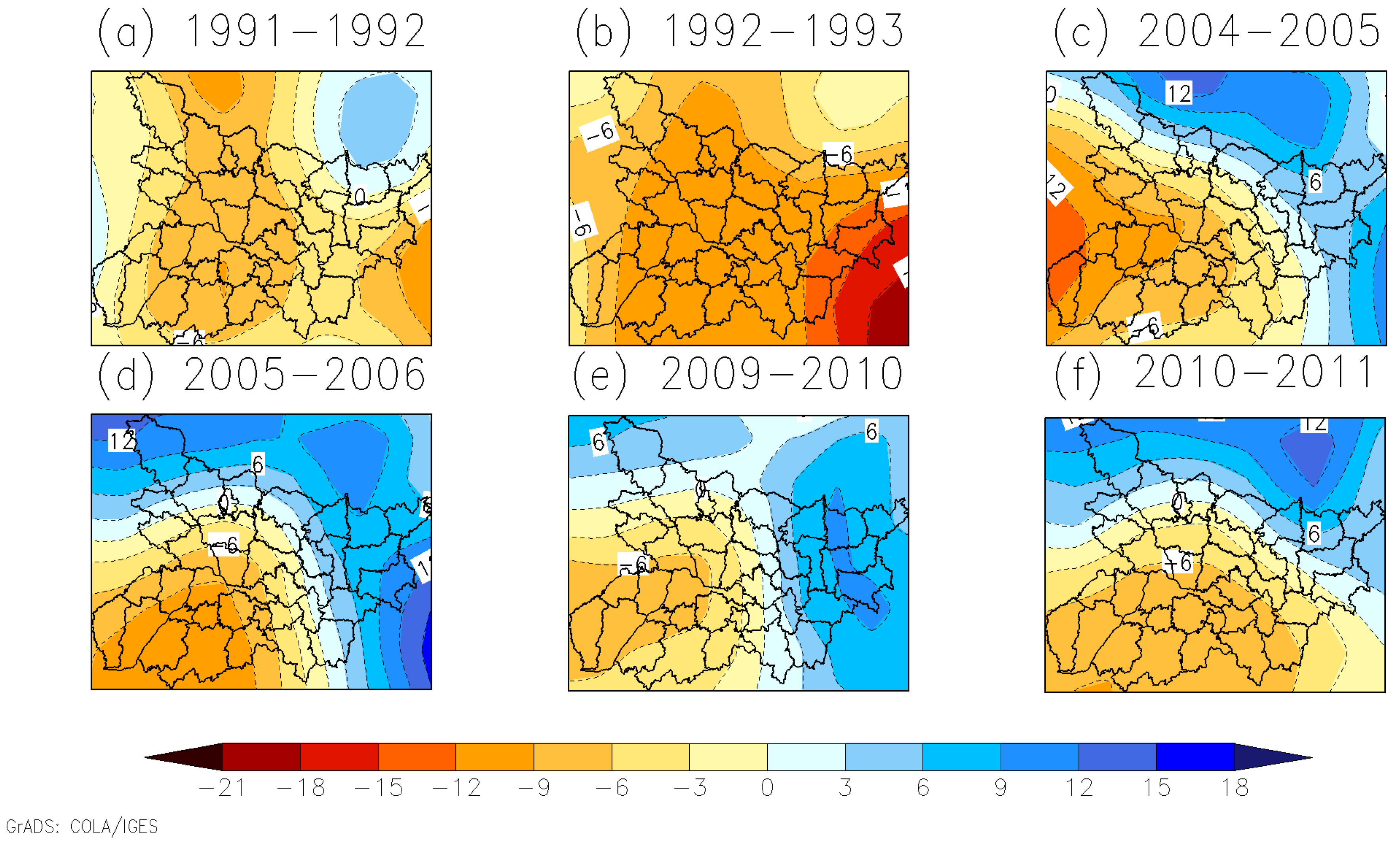
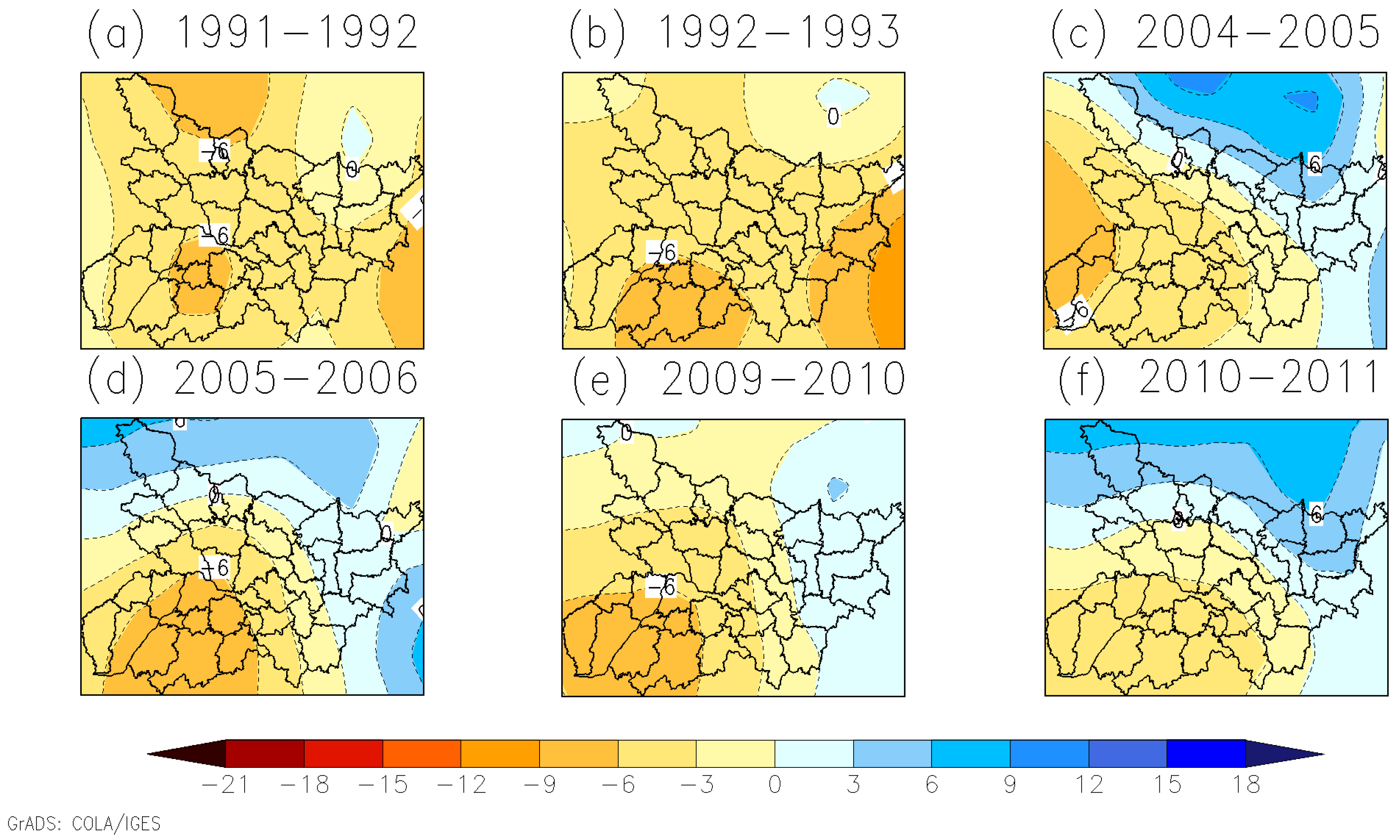
Negative anomalies of rainfall and soil moisture (Figure 3, Figure 4 and Figure 5) were observed during the JAS season for all the low productivity years. In comparison to seasonal rainfall and soil moisture in JAS, Figure 6 for NDJ and Figure 7 for MAM showed a little decrease in the magnitude of the anomaly. Figure 5a,b clearly reflects the significant scarcity of rainfall and soil moisture in the JAS season for all the event years. All the event years selected in this study had a severer than −10% anomalous deviation in rice productivity. During the first event year, 1991–1992 as shown in Table 1, significant El Niño phase persisted for three seasons starting in MJJ of 1991 and encompassed throughout the rice-growing seasons, especially Kharif and Rabi. Therefore, rainfall anomaly in JAS (Figure 3a) and soil moisture anomaly in JAS, NDJ and MAM season of 1991–1992 remained highly negative (Figure 4a, Figure 6a and Figure 7a).
In the second declining event of 1992–1993, the El Niño phase of ENSO affected the rainfall during MAM of 1991 to JJA of 1992. It directly impacted the sowing season (Figure 3a and Figure 4a) and it led to the total decline in the yield by −29.76%. Failure of southwest monsoonal rainfall reduced the soil moisture content not only in highly productive districts but also in other parts as well (Figure 3b, Figure 4b, Figure 6b and Figure 7b).
In the case of third and fourth events of 2004–2005 and 2005–2006 respectively, the commencement of the El Niño phase in JJA of 2004 survived for several seasons and ended in MAM of 2005. This affected monsoonal rainfall and soil moisture in almost all the rice-producing districts in the state (Figure 3c, Figure 4c, Figure 6c and Figure 7c). The rainfall and soil moisture were scarce even at the beginning of the sowing season for 2005–2006 (Figure 3d), which led to the decline of rice productivity for 2004–2005 and 2005–2006, respectively. Soil moisture content was low in JAS (Figure 4c,d) but its spatial distribution expanded in NDJ and MAM (Figure 6c,d and Figure 7c,d).
The sixth low yield event of 2009–2010 had after-effects of flood in 2008 due to a breach of the embankment in Nepal [75]. As already discussed in Section 1, Bihar is a rainfed region and rainfed regions of India are affected by extreme hydrological events like some other exceptional regions across the globe [76,77]. Another cause for the decline was indicated by ONI (JJA of 2009 to JJA of 2009) and SOI (MAM 2009 to JJA 2009) as shown in Table 1. These conditions resulted in low rainfall and soil moisture from JAS of 2009 to other succeeding rice growing seasons. Figure 5 for composite rainfall and soil moisture cases and Figure 3e, Figure 4e, Figure 6e and Figure 7e clearly showed that anomalies of rainfall and soil moisture in JAS, NDJ, and MAM for all the event years with severer than −10% decline were negative. This clearly demonstrated that the scarcity of water leads to a decline in rice productivity. Moreover, some in-depth study will be highly important to understand the underlying complexities related to atmospheric circulation in this fifth event year.
In the sixth event of 2010–2011, declined rainfall (Figure 3f) was the consequence of the prevalence of El Niño from SON of 2009 to MAM of 2010. Eventually, La Niña developed during JAS of 2010 to MAM of 2011, the rainfall did not recover. It might be related to some local atmospheric dynamics that need further investigation.

3.3. Temperature

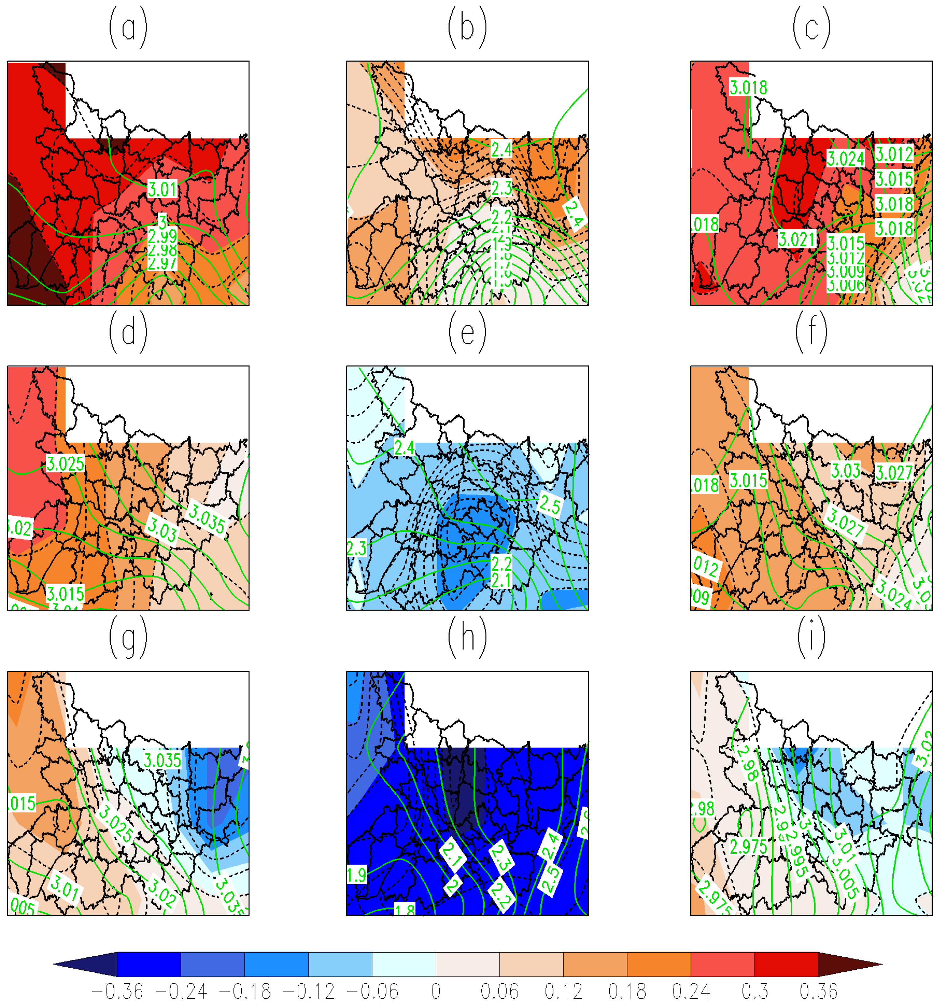
Composite of all the years with severer than −10% anomalous percentage deviation in the productivity of rice showed an increase in the maximum surface air temperature of all the seasons (Figure 8a,c). The increase in the maximum temperature was found comparatively much higher than normal for all the rice-growing seasons. The least increase in maximum temperature was observed in the NDJ season. As shown in Figure 8a,d,e, it was found that an increase of temperature during the JAS season remained consistent among all the variants of temperature and a decline in the seasonal minimum temperature was profound in the NDJ season for mean and minimum temperature. Therefore, the connection between an increase in the temperature and its connection with the decline of rice productivity was further investigated and discussed here in this Section 3.3. Event wise prevalence of maximum and minimum temperature in different seasons is shown in Figures S1 and S2.
As far as SST is concerned, the composite anomalies in the Pacific Ocean indicated an El Niño event with prevailing anomalies of outgoing longwave radiation (hereafter OLR) and zonal wind (Figure 9). In the case of particular event years with severer than −10% anomalous deviation, it was observed that the seasonal maximum temperature pattern in Bihar followed the ONI index (Figure S1). In the case of the El Niño event, the maximum temperature was found above the climatology (Figure S1) and the minimum temperature falls below the climatology (Figure S2). Therefore, the range of daily temperature variation increased in all the El Niño event years.
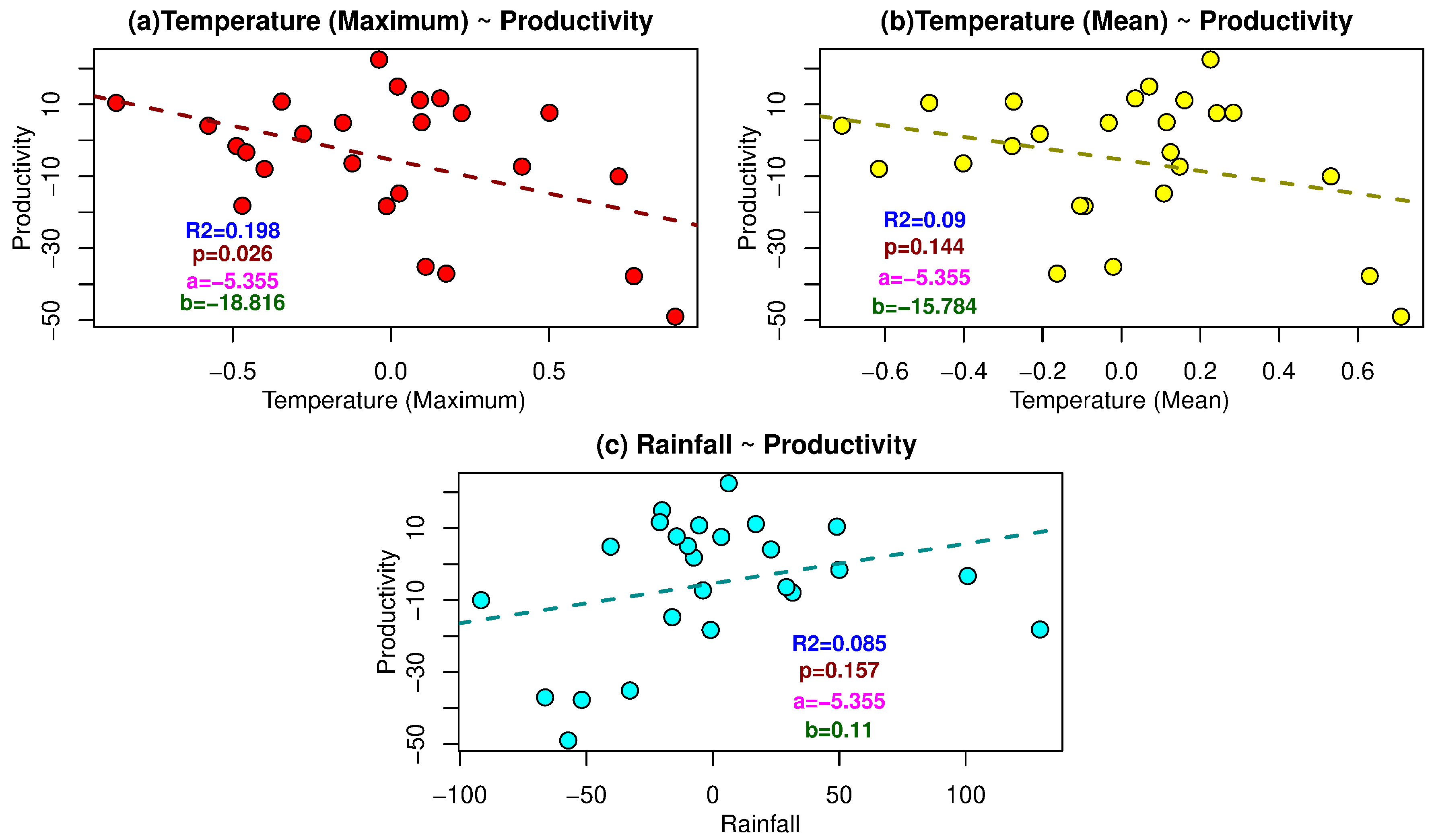
We calculated the association of climatic variables over Bihar with rice productivity and found the dominance of maximum temperature in it. Over the period 1991–1992 to 2014–2015, a high magnitude of the decline in productivity (obtained through slope value) and the good association of anomalous maximum (significant at 95% level of significance) and mean temperature with rice productivity was found. Figure 10a,b show that one unit of change in maximum (mean) temperature leads to a decline of 18.816% (15.784%) rice productivity. Interestingly, monotonous trend results (Table 2) also expressed the highest positive magnitude (b in Figure 10a) of the increase in maximum temperature (significant at 99% level). On the basis of these obtained results, it becomes evident that the increase in temperature in Bihar causes a decline in the productivity of rice. Therefore, the prevailing conditions in the Indo-Pacific region leading to the increase in temperature are not favorable for rice productivity in Bihar.
Each variant of temperature showed a significant increasing monotonous trend at the 99% level. Trend results of climatic variables with productivity showed strong relation with maximum temperature (p-value 0.026) followed by mean temperature (p-value 0.144) and rainfall (p-value 0.157) (Figure 10). As discussed above, we found the consistency with the increase in temperature and its association with productivity was comparatively stronger than rainfall. Some flood events due to exceptionally high rainfall events or breaking of the embankment caused its relationship to become a little lenient. Though, the monotonously decreasing rainfall and the increasing temperature was a real worry for rice productivity in view of the one to one relationship between productivity and climatic variables (Figure 10a,c).

4. Discussion

In this study, it was observed that climate factors like rainfall, temperature, soil moisture and Indo-Pacific climate variability played a dominant role in deciding the rice productivity in Bihar. On the basis of the event wise scrutiny of the impact of prevailing large-scale mechanism on the local climatic conditions, it was worthwhile to note that rainfall and soil moisture [78] behaved according to the role played by the discerned climate indices (ONI, Niño 3 and SOI) with significantly high correlation with rice productivity. Thereby, scarcity of the rainfall and soil moisture was found highly associated with the signals provided by climate indices. During 2010–2011, a shortfall of more than 20% rainfall was observed and all the districts were declared drought-prone [79]. The sowing season was affected due to the late onset of monsoon by 2–3 weeks [80].
The literature discussed in Section 1 of this study revealed the teleconnection and its association with rainfall. However, due to fragility of the crop to temperature, it was important to look into the behavior of temperature also and we found a high association with maximum temperature in the case of Bihar. Effective adaptation strategies must be adopted to save the water received through rain so that the crop becomes resilient to the impact of climate variability [81,82,83].
Capturing the teleconnection signal in a quick and simple manner was through the composite map of the events and visualization of spatial patterns through it. Teleconnection signals captured through the composite anomaly map of SST, OLR and zonal wind reflected the effect of Pacific warming during the event years (Figure 9). However, this is not always a guarantee for every case due to its generalized nature. Therefore, we captured the event wise scenario for event years with severer than −10% deviation. While mapping the high to low productivity districts in Bihar, we found that most of the high productivity districts are located in the southern part of Bihar.
A very important study revealed the vulnerability of upper Ganges to drought and lower Ganges to flood due to high rainfall in lower Ganges [36]. Contrary to Asada and Matsumoto (2009), we found homogeneity in the trend of rainfall across Bihar during the event years. Anomalies of soil moisture and rainfall were directly proportional to each other in the same season (JAS) as well as in later seasons (NDJ and MAM). Therefore, the substitution of rainfall was made with soil moisture for the NDJ and MAM season. Identification and monitoring of the vulnerable zones using remote sensing data may prove very helpful to mitigate the loss of rice productivity due to flood [84,85].
A most important phenomenon observed in the study was the excessive maximum temperature during the declining productivity years. This fact of increasing temperature and its impact was highlighted in many previous studies on India [86] and the association of maximum temperature as observed in Figure 8a–c was an interesting case for Bihar also. This important finding in the present study was supported by the temperature based sensitivity experiment on rice production in Indian cases and revealed the negative impact on rice due to an increase in temperature [87].
Persistent above normal temperature, lack of rainfall and soil moisture (especially in the districts with more than 1500 kg/ha rice productivity) are identified as the important factors in cases of severe loss in rice productivity. A very strong association of persisting conditions are found in high positive (negative) association with the ONI and Niño 3 (SOI). Bihar produces a large part of Indian rice and therefore vulnerability of rice productivity needs to be addressed earnestly. A lot of uncertainties in the case of the South Asia Monsoon increase the vulnerability [88], hence there is still a way to go for predicting the Monsoon with high precision [89]. In the future, some other study at the pan-Bihar level by considering different constraints to the rice productivity will be relevant to look into the intensity of the impact of different elements, i.e., physical, chemical, and biological.

5. Conclusions

This study examined rainfall, temperature, soil moisture, and Indo-Pacific climate indices and their relation with rice productivity in Bihar. Results are based on statistical methods like PPMC, Partial Correlation, Mann Kendall Test and Linear Regression Model. Both the methods, i.e., PPMC and Partial Correlation, had their own significance and in the present study, both of them were used as a filtration mechanism to identify the most significant association of climate factors and climate indices with rice productivity. Based on the event wise trend of rainfall in different districts of Bihar, it can be concluded that the majority of climate indices in the Pacific Ocean had direct relation. Whereas, climate indices in the Indian Ocean had an indirect relation. There was a high impact on the JAS seasonal rainfall and temperature with respect to the occurrence of the prevailing intensity and timing of the Indo-Pacific climate indices. Scarcity of rainfall, low soil moisture and persistence of high temperature (especially maximum temperature) are found to be the primary consequences of the prevailing ONI, Niño 3 and SOI leading to the decline in rice productivity.
In general, Partial Correlation of DJF season for ONI, Niño 3, DMI, and TNI were found uniformly good and in Particular Partial Correlation value for AMJ season was comparatively higher for ONI, SOI and Niño 3 (−0.739, 0.731 and 0.677 respectively). However, highlighting that high correlation does not mean the correlation is significantly different from zero, we calculated the identified significant high correlation as tabulated in Table 1. Here, it can be summarized that along with the impact on rainfall and soil moisture, an increase in the range of temperature was also found in the years of declining productivity. With respect to temperature, the Linear Regression revealed the close association of maximum temperature with productivity during the study period. There appeared weak PPMC for DMI and MI with rice productivity in Bihar though Partial Correlation value of DMI improved in JJA season (−0.499) but it was not significant and the Monsoon index remained weak. Moreover, the impact on regional atmospheric circulation due to intra-seasonal variability and some hazards like breaking of embankments in Nepal do affect the productivity of rice. Therefore, it should be noted that there exists a lot of complexities in the South West Monsoon system in India and early identification of which was a highly complicated task. However, the prediction of such intra-seasonal variation can be of benefit in understanding the impact on rice productivity in Bihar. It would be interesting to study the episodes causing intra-seasonal variation and further studies will be highly important for sustainable livelihood systems.

Supplementary Materials

The following are available online at https://www.mdpi.com/2071-1050/12/17/7023/s1, Figure S1: Mean maximum temperature anomaly for all the years (as per Table 1) with severer than −10% anomalous percentage deviation in rice productivity of Bihar. Map (a) to (f) is JAS season, (g) to (l) for NDJ season and (m) to (r) for MAM. (Figure was created using a free software Grid Analysis and Display System (hereafter GrADS) version 2.0.2 (http://cola.gmu.edu/grads/downloads.php), Figure S2: Mean minimum temperature anomaly for all the years (as per Table 1) with severer than −10% anomalous percentage deviation in rice productivity of Bihar. Map (a) to (f) is JAS season, (g) to (l) for NDJ season and (m) to (r) for MAM. (Figure was created using a free software GrADS version 2.0.2 (http://cola.gmu.edu/grads/downloads.php), Table S1: General PPMC result for the period 1991–1992 to 2014–2015. Coloumn (row) in the table represents the climate indices (seasons of the climate indices). Values in bold format are significant at 90% level of significance and values highlighted with red color represent the value exceeding >0.5 and < −0.5, Table S2: Particular PPMC for all the six event years. Coloumn (row) in the table represents the uncontrolled (controlled) climate indices in different seasons. Values in bold format are significant at 90% level of significance and values highlighted with red color represent the value exceeding >0.5 and < −0.5, Table S3: General Partial Correlation for the period 1991–1992 to 2014–2015. Coloumn (row) in the table represents the uncontrolled (controlled) climate indices in different seasons. Values in bold format are significant at 90% level of significance and values highlighted with red color represent the value exceeding >0.5 and < −0.5. Table S4: Particular Partial Correlation for all the six event years. Coloumn (row) in the table represents the uncontrolled (controlled) climate indices in different seasons. Values in bold format are significant at 90% level of significance and values highlighted with red color represent the value exceeding >0.5 and < −0.5.

Author Contributions

N.S. and A.S. contributed equally and conceptualized the central idea, carried out the analysis, drew all the figures and wrote the paper. S.B. suggested important methods for carrying out the research. S.B., T.S., L.S., S.N., W.D. and R.A. edited and commented on the manuscript. M.Y., R.B.S. and K.T. provided guidance for the analysis. All authors have read and agreed to the published version of the manuscript.

Funding

This work has been supported by JSPS Kakenhi Grant-in-Aid id:18F18360

Acknowledgments

The rice production data were obtained from the Economic Survey Report of Finance Department, Government of Bihar, Patna and Handbook of Statistics Directorate of Rice Development, Department of Agriculture & Co-Operation, Ministry of Agriculture, Government of India, Patna. The authors are thankful to the India meteorological department for providing the high resolution gridded temperature and rainfall data. SST and Soil Moisture data were provided by NOAA/ESRL PSD, Boulder, Colorado, USA (https://www.esrl.noaa.gov/psd/data/gridded/data.noaa.oisst.v2.html and https://www.esrl.noaa.gov/psd/data/gridded/data.cpcsoil.html). Authors are also thankful to IRI Data Library for making available the NOAA NCEP-NCAR CDAS-1 daily zonal wind data and NOAA NCEP CPC GLOBAL daily OLR data. Data of different climate indices were provided by JAMSTEC, Asia-Pacific Data-Research Center of IPRC and NOAA. All the figures showing the climatic variable in this study were drawn by GrADS Version 2.0.2 (http://cola.gmu.edu/grads/downloads.php). ArcGIS 10.2.1.3497 for Desktop (https://www.esri.com) was used to draw a Locational map and Rice productivity map. SPSS Version 22.0 was used to calculate the PPMC and Partial Correlation. NCAR Command Language was used to draw linear and bar graphs. At present, Netrananda Sahu is working as a JSPS Postdoc Fellow at DPRI, Kyoto University. We are thankful to JSPS (ID No. P18360), Japan.

Conflicts of Interest

The authors declare that they have no competing interest.

Abbreviations

The following abbreviations are used in this manuscript:
DJFDecember-January-February
JFMJanuary-February-March
FMAFebruary-March-April
AMJAugust-May-June
NDJNovember-December-January
MAMMarch-April-May
MJJMay-June-July
JASJuly-August-September
ASOAugust-September-October
GOSATGreenhouse Gases Observing Satellite
ENSOEl Niño-Southern Oscillation
SSTSea Surface Temperature
SOISouthern Oscillation Index
EMIEl Niño Modoki Index
DMIDipole mode index
TNITrans Niño Index
MIMonsoon Index
IODIndian Ocean Dipole
PPMCPearson’s Product Moment Correlation
OLROutgoing Longwave Radiation
JAMSTECJapan Agency for Marine-Earth Science and Technology
CGDClimate and Global Dynamics Laboratory
AUTamil Nadu Agricultural University
DRDPATDirectorate of Rice Development Patna
ONIOcean Niño Index
ICARIndian Council of Agricultural Research
TNIRRIInternational Rice Research Institute
DESDirectorate of Economics and Statistics
WAOBWorld Agricultural Outlook Board
UNICEFUnited Nations Children’s Fund
NCARNational Center for Atmospheric Research
GrADSGrid Analysis and Display System

References

  1. Whetton, P.; Rutherfurd, I. Historical ENSO teleconnections in the eastern hemisphere. Clim. Chang. 1994, 28, 221–253. [Google Scholar] [CrossRef]
  2. Selvaraju, R. Impact of El Niño-southern oscillation on Indian foodgrain production. Int. J. Climatol. 2003, 23, 187–206. [Google Scholar] [CrossRef]
  3. Abbas, S.; Mayo, Z.A. Impact of temperature and rainfall on rice production in Punjab, Pakistan. Environ. Dev. Sustain. 2020, 121, 1–13. [Google Scholar] [CrossRef]
  4. Kellner, O.; Niyogi, D. Climate Variability and the U.S. Corn Belt: ENSO and AO Episode-Dependent Hydroclimatic Feedbacks to Corn Production at Regional and Local Scales. Earth Interact. 2015, 19, 1–32. [Google Scholar] [CrossRef]
  5. Panda, A.; Sahu, N.; Behera, S.; Sayama, T.; Sahu, L.; Avtar, R.; Singh, R.B.; Yamada, M. Impact of Climate Variability on Crop Yield in Kalahandi, Bolangir, and Koraput Districts of Odisha, India. Climate 2019, 7, 126. [Google Scholar] [CrossRef] [Green Version]
  6. Mishra, A.K.; Avm, I.; Das, N.N.; Khedun, C.P.; Singh, V.P.; Sivakumar, B.; Hansen, J.W. Anatomy of a local-scale drought: Application of assimilated remote sensing products, crop model, and statistical methods to an agricultural drought study. J. Hydrol. 2015, 526, 15–29. [Google Scholar] [CrossRef]
  7. Bagagnan, A.R.; Ouedraogo, I.; Fonta, W.M. Perceived Climate Variability and Farm Level Adaptation in the Central River Region of The Gambia. Atmosphere 2019, 10, 423. [Google Scholar] [CrossRef] [Green Version]
  8. Ashok, K.; Guan, Z.; Saji, N.H.; Yamagata, T. Individual and Combined Influences of ENSO and the Indian Ocean Dipole on the Indian Summer Monsoon. J. Clim. 2004, 17, 3141–3155. [Google Scholar] [CrossRef]
  9. Sahu, N.B.S.; Ratnam, J.V.; Silva, R.V.; Parhi, P.; Duan, W.; Takara, K.; Singh, R.B.; Yamagata, T. El Nino Modoki connection to extremely-low streamflow of the Paranaiba River in Brazil. Clim. Dyn. 2014, 2014, 1509–1516. [Google Scholar] [CrossRef]
  10. Nayak, S.; Mandal, M. Examining the impact of regional land use and land cover changes on temperature: The case of Eastern India. Spat. Inf. Res. 2019, 27, 601–611. [Google Scholar] [CrossRef]
  11. Nayak, S.; Mandal, M. Impact of land use and land cover changes on temperature trends over India. Land Use Policy 2019, 89, 104238. [Google Scholar] [CrossRef]
  12. Anderson, W.B.; Seager, R.; Baethgen, W.; Cane, M.; You, L. Synchronous crop failures and climate-forced production variability. Sci. Adv. 2019, 5, 7. [Google Scholar] [CrossRef] [PubMed] [Green Version]
  13. Sahu, N.; Yamashiki, Y.; Behera, S.; Takara, K.; Yamagata, T. Large Impacts of Indo-Pacific Climate Modes on the Extreme Streamflows of Citarum River in Indonesia. J. Glob. Environ. Eng. 2012, 17, 1–8. [Google Scholar]
  14. Sahu, N.; Singh, R.B.; Kumar, P.; Silva, R.V.D.; Behera, S.K. La Niña Impacts on Austral Summer Extremely High-Streamflow Events of the Paranaíba River in Brazil. Adv. Meteorol. 2013, 2013, 461693. [Google Scholar] [CrossRef]
  15. Ubilava, D.; Abdolrahimi, M. The El Niño impact on maize yields is amplified in lower income teleconnected countries. Environ. Res. Lett. 2019, 14, 054008. [Google Scholar] [CrossRef]
  16. Roberts, M.G.; Dawe, D.; Falcon, W.P.; Naylor, R.L. El Niño-Southern Oscillation Impacts on Rice Production in Luzon, the Philippines. J. Appl. Meteorol. Climatol. 2009, 48, 1718–1724. [Google Scholar] [CrossRef]
  17. Kumar, K.K.; Kumar, K.R.; Ashrit, R.G.; Deshpande, N.R.; Hansen, J.W. Climate impacts on Indian agriculture. Int. J. Climatol. 2004, 24, 1375–1393. [Google Scholar] [CrossRef]
  18. Iskandar, I.; Mardiansyah, W.; Lestari, D.O.; Masumoto, Y. What did determine the warming trend in the Indonesian sea? Prog. Earth Planet. Sci. 2020, 7, 1–11. [Google Scholar] [CrossRef]
  19. Ropelewski, C.F.; Jones, P.D. An Extension of the Tahiti-Darwin Southern Oscillation Index. Mon. Weather Rev. 1987, 115, 2161–2165. [Google Scholar] [CrossRef] [Green Version]
  20. Wang, B.; Fan, Z. Choice of South Asian Summer Monsoon Indices. Bull. Am. Meteorol. Soc. 1999, 80, 629–663. [Google Scholar] [CrossRef] [Green Version]
  21. Ashok, K.; Behera, S.K.; Rao, S.A.; Weng, H.; Yamagata, T. El Niño Modoki and its possible teleconnection. J. Geophys. Res. 2007, 112. [Google Scholar] [CrossRef]
  22. Trenberth, K. The Climate Data Guide: Nino SST Indices (Nino 1+2, 3, 3.4, 4; ONI and TNI). In Climate Data Guide; UCAR: Boulder, CO, USA, 2020. [Google Scholar]
  23. Liu, W.; Zhu, S.; Huang, Y.; Wan, Y.; Wu, B.; Liu, L. Spatiotemporal variations of drought and their teleconnections with large-scale climate indices over the Poyang Lake Basin, China. Sustainability 2020, 12, 3526. [Google Scholar] [CrossRef]
  24. Sahu, N.; Panda, A.; Nayak, S.; Saini, A.; Mishra, M.; Sayama, T.; Sahu, L.; Duan, W.; Avtar, R.; Behera, S.; et al. Impact of Indo-Pacific Climate Variability on High Streamflow Events in Mahanadi River Basin, India. Water 2020, 12, 1952. [Google Scholar] [CrossRef]
  25. Mayer, D.A.; Weisberg, R.H. El Niño-Southern Oscillation-related ocean-atmosphere coupling in the western equatorial Pacific. J. Geophys. Res. Ocean. 1998, 103, 18635–18648. [Google Scholar] [CrossRef]
  26. Yamagata, T.; Morioka, Y.; Behera, S. Indo-Pacific Climate Variability and Predictability; World Scientific: Singapore, 2016. [Google Scholar]
  27. Yuan, C.; Yamagata, T. Impacts of IOD, ENSO and ENSO Modoki on the Australian Winter Wheat Yields in Recent Decades. Sci. Rep. 2015, 5, 17252. [Google Scholar] [CrossRef] [Green Version]
  28. Soora, N.K.; Aggarwal, P.K.; Saxena, R.; Rani, S.; Jain, S.; Chauhan, N. An assessment of regional vulnerability of rice to climate change in India. Clim. Chang. 2013, 118, 683–699. [Google Scholar] [CrossRef]
  29. Chen, S.; Chen, X.; Xu, J. Assessing the impacts of temperature variations on rice yield in China. Clim. Chang. 2016, 138, 191–205. [Google Scholar] [CrossRef]
  30. Stuecker, M.F.; Tigchelaar, M.; Kantar, M.B. Climate variability impacts on rice production in the Philippines. PLoS ONE 2018, 13, 8. [Google Scholar] [CrossRef]
  31. Koide, N.; Robertson, A.W.; Ines, A.V.; Qian, J.; Dewitt, D.G.; Lucero, A. Prediction of Rice Production in the Philippines Using Seasonal Climate Forecasts. J. Appl. Meteorol. Climatol. 2013, 52, 552–569. [Google Scholar] [CrossRef] [Green Version]
  32. De Datta, S.K. Principles and Practices of Rice Production; John Wiley & Sons: Hoboken, NJ, USA, 1981. [Google Scholar]
  33. TNAU. Water Management; Tamil Nadu Agricultural University, Directorate of Extension Education Tamil Nadu Agricultural University Coimbatore—641 003: Coimbatore, India, 2015. [Google Scholar]
  34. DRDPAT. Rice—A Status Paper; Directorate of Rice Development; Department of Agriculture & Co-Operation, Ministry of Agriculture, Government of India: Patna, India, 2014.
  35. IRRI. Rice Almanac: Source Book for One of the Most Economic Activities on Earth; Maclean, J., Dawe, D., Hardy, B., Hettel, G.E., Eds.; CABI Publishing: Los Baños, Philippines, 2002. [Google Scholar]
  36. Asada, H.; Matsumoto, J. Effects of rainfall variation on rice production in the Ganges-Brahmaputra Basin. Clim. Res. 2009, 38, 249–260. [Google Scholar] [CrossRef] [Green Version]
  37. Duan, W.; He, B.; Sahu, N.; Luo, P.; Nover, D.; Hu, M.; Takara, K. Spatiotemporal variability of Hokkaido’s seasonal precipitation in recent decades and connection to water vapour flux. Int. J. Climatol. 2017, 37, 3660–3673. [Google Scholar] [CrossRef]
  38. Finance Department. Economic Survey 2015–2016; Finance Department, Government of Bihar: Patna, India, 2016.
  39. ODCO. Census of India, Provisional Population Totals; Office of the Director of Census Operations: Patna, India, 2011.
  40. DES. Agricultural Statistics at a Glance; Directorate of Economics and Statistics, Government of India: New Delhi, India, 2011.
  41. Singh, S.K.; Singh, K.M.; Singh, R.P.; Kumar, A.; Kumar, U. Impact of Rainfall on Agricultural Production in Bihar: A Zone-Wise Analysis. Environ. Ecol. 2014, 32, 1571–1576. [Google Scholar]
  42. Haris, A.A.; Biswas, S.; Chhabra, V. Climate change impacts on productivity of rice (Oryza sativa) in Bihar. Indian J. Agron. 2014, 55, 295–298. [Google Scholar]
  43. Tesfaye, K.; Aggarwal, P.; Mequanint, F.; Shirsath, P.; Stirling, C.; Khatri-Chhetri, A.; Rahut, D. Climate Variability and Change in Bihar, India: Challenges and Opportunities for Sustainable Crop Production. Sustainability 2017, 9, 1998. [Google Scholar] [CrossRef] [Green Version]
  44. Khan, M.A.; Tahir, A.; Khurshid, N.; ul Husnain, M.I.; Ahmed, M.; Boughanmi, H. Economic effects of climate change-induced loss of agricultural production by 2050: A case study of Pakistan. Sustainability 2020, 12, 1216. [Google Scholar] [CrossRef] [Green Version]
  45. ICAR. State-Specific Technological Interventions for Higher Agricultural Growth; Indian Council of Agriculture Research: New Delhi, Indian, 2007.
  46. WAOB. Major World Crop Areas and Climatic Profiles; World Agricultural Outlook Board, United States Department of Agriculture: Washington, DC, USA, 1994.
  47. Naylor, R.; Falcon, W.; Rochberg, D.; Wada, N. Using El Niño/Southern Oscillation Climate Data to Predict Rice Production in Indonesia. Clim. Chang. 2001, 50, 255–265. [Google Scholar] [CrossRef]
  48. Anderson, W.B.; Seager, R.; Baethgen, W.; Cane, M. Crop production variability in North and South America forced by life-cycles of the El Niño Southern Oscillation. Agric. For. Meteorol. 2017, 239, 151–165. [Google Scholar] [CrossRef] [Green Version]
  49. Ashok, K.; Yamagata, T. The El Niño with a difference. Nature 2009, 461, 481–484. [Google Scholar] [CrossRef]
  50. DRDPAT. Rice in India—A Handbook of Statistics 2007; Directorate of Rice Development, Department of Agriculture & Co-Operation, Ministry of Agriculture, Government of India: Patna, India, 2007.
  51. Finance Department. Economic Survey 2013–2014; Finance Department, Government of Bihar: Patna, India, 2014.
  52. Finance Department. Economic Survey 2014–2015; Finance Department, Government of Bihar: Patna, India, 2015.
  53. Finance Department. Economic Survey 2016–2017; Finance Department, Government of Bihar: Patna, India, 2017.
  54. El-Maayar, M.; Lange, M. A Methodology to Infer Crop Yield Response to Climate Variability and Change Using Long-Term Observations. Atmosphere 2013, 4, 365–382. [Google Scholar] [CrossRef] [Green Version]
  55. Pai, D.S.; Sridhar, L.; Rajeevan, M.; Sreejith, O.P.; Satbhai, N.S.; Mukhopadyay, B. Analysis of the daily rainfall events over India using a new long period (1901–2010) high resolution (0.25° × 0.25°) gridded rainfall data set. MAUSAM 2014, 65, 1–18. [Google Scholar] [CrossRef]
  56. Srivastava, A.K.; Rajeevan, M.; Kshirsagar, S.R. Development of a high resolution daily gridded temperature data set (1969–2005) for the Indian region. Atmos. Sci. Lett. 2009, 10, 249–254. [Google Scholar] [CrossRef]
  57. Dool, H.V.D.; Huang, J.; Fan, Y. Performance and analysis of the constructed analogue method applied to U.S. soil moisture over 1981–2001. J. Geophys. Res. 2003, 108. [Google Scholar] [CrossRef]
  58. Reynolds, R.W.; Smith, T.M.; Liu, C.; Chelton, D.B.; Casey, K.S.; Schlax, M.G. Daily High-Resolution-Blended Analyses for Sea Surface Temperature. J. Clim. 2007, 20, 5473–5496. [Google Scholar] [CrossRef]
  59. Kalnay, E.; Kanamitsu, M.; Kistler, R.; Collins, W.; Deaven, D.; Gandin, L.; Iredell, M.; Saha, S.; White, G.; Woollen, J.; et al. The NCEP/NCAR 40-Year Reanalysis Project. Bull. Am. Meteorol. Soc. 1996, 77, 437–471. [Google Scholar] [CrossRef] [Green Version]
  60. Liebmann, B.; Smith, C.A. Description of a complete (interpolated) outgoing longwave 461 radiation dataset. Bull. Am. Meteorol. Soc. 1996, 77, 1275–1277. [Google Scholar]
  61. Mukherjee, A.; S-y, W.; Promchote, P. Examination of the Climate Factors That Reduced Wheat Yield in Northwest India during the 2000s. Water 2019, 11, 343. [Google Scholar] [CrossRef] [Green Version]
  62. Trenberth, K.E.; Stepaniak, D.P. Indices of El Niño Evolution. J. Clim. 2001, 14, 1697–1701. [Google Scholar] [CrossRef] [Green Version]
  63. Ashok, K.; Guan, Z.; Yamagata, T. Impact of the Indian Ocean dipole on the relationship between the Indian monsoon rainfall and ENSO. Geophys. Res. Lett. 2001, 28, 4499–4502. [Google Scholar] [CrossRef] [Green Version]
  64. Izumo, T.; Vialard, J.; Lengaigne, M.; Montegut, C.D.; Behera, S.K.; Luo, J.; Cravatte, S.; Masson, S.; Yamagata, T. Influence of the state of the Indian Ocean Dipole on the following year’s El Niño. Nat. Geosci. 2010, 3, 168–172. [Google Scholar] [CrossRef] [Green Version]
  65. Li, Z.; Cai, W.; Lin, X. Dynamics of changing impacts of tropical Indo-Pacific variability on Indian and Australian rainfall. Sci. Rep. 2016, 6, 31767. [Google Scholar] [CrossRef]
  66. Saji, N.H.; Goswami, B.N.; Vinayachandran, P.N.; Yamagata, T. A dipole mode in the tropical Indian Ocean. Nature 1999, 401, 360–363. [Google Scholar] [CrossRef] [PubMed]
  67. JAMSTEC. SST DMI Dataset (Monthly from 1870 to Present); JAMSTEC: Kanagawa, Japan, 2017.
  68. Achuthavarier, D.; Krishnamurthy, V.; Kirtman, B.P.; Huang, B. Role of the Indian Ocean in the ENSO-Indian Summer Monsoon Teleconnection in the NCEP Climate Forecast System. J. Clim. 2012, 25, 2490–2508. [Google Scholar] [CrossRef]
  69. Trenberth, K.E. The Definition of El Niño. Bull. Am. Meteorol. Soc. 1997, 78, 2771–2777. [Google Scholar] [CrossRef] [Green Version]
  70. Lobell, D.B.; Hammer, G.L.; Mclean, G.; Messina, C.; Roberts, M.J.; Schlenker, W. The critical role of extreme heat for maize production in the United States. Nat. Clim. Chang. 2013, 3, 497–501. [Google Scholar] [CrossRef]
  71. Sahu, N.; Robertson, A.W.; Boer, R.; Behera, S.; DeWitt, D.G.; Takara, K.; Kumar, M.; Singh, R.B. Probabilistic seasonal streamflow forecasts of the Citarum River, Indonesia, based on general circulation models. Stoch. Environ. Res. Risk Assess. 2017, 31, 1747–1758. [Google Scholar] [CrossRef]
  72. Mann, H.B. Non-parametric tests against trend. Econometrica 1945, 13, 163–171. [Google Scholar] [CrossRef]
  73. Sen, P.K. Estimates of the regression coefficient based on Kendall’s tau. J. Am. Stat. Assoc. 1968, 63, 1379–1389. [Google Scholar] [CrossRef]
  74. Theil, H. A rank-invariant method of linear and polynomial regression analysis, Part I. Proc. R. Neth. Acad. Arts Sci. 1950, 53, 386–392. [Google Scholar]
  75. Kumar, S.; Sahdeo, A.; Guleria, S. Bihar Floods: 2007 (A Field Report); Technical Report; National Institute of Disaster Management, Ministry of Home Affairs: New Delhi, India, 2013.
  76. Auffhammer, M.; Ramanathan, V.; Vincent, J.R. Climate change, the monsoon, and rice yield in India. Clim. Chang. 2011, 111, 411–424. [Google Scholar] [CrossRef]
  77. Wei, T.; Zhang, T.; de Bruin, K.; Glomrød, S.; Shi, Q. Extreme weather impacts on maize yield: The case of Shanxi Province in China. Sustainability 2017, 9, 41. [Google Scholar] [CrossRef] [Green Version]
  78. Mishra, A.; Vu, T.; Veettil, A.V.; EntekhabI, D. Drought monitoring with soil moisture active passive (SMAP) measurement. J. Hydrol. 2017, 552, 620–632. [Google Scholar] [CrossRef]
  79. Finance Department. Economic Survey 2010–2011; Finance Department, Government of Bihar: Patna, India, 2011.
  80. Bhatnagar, M.K.; Faruqi, A.A.; Singh, U.P.; Sharma, S.C.; Khurana, S.; Khanna, D.; Chand, G. (Eds.) Annual Report 2010; India Meteorological Department: New Delhi, India, 2011.
  81. Thakur, A.K.; Kassam, A.; Stoop, W.A.; Uphoff, N. Modifying rice crop management to ease water constraints with increased productivity, environmental benefits, and climate-resilience. Agric. Ecosyst. Environ. 2016, 235, 101–104. [Google Scholar] [CrossRef]
  82. Pray, C.; Nagarajan, L.; Li, L.; Huang, J.; Hu, R.; Selvaraj, K.N.; Napasintuwong, O.; Chandra Babu, R. Potential impact of biotechnology on adaption of agriculture to climate change: The case of drought tolerant rice breeding in Asia. Sustainability 2011, 3, 1723–1741. [Google Scholar] [CrossRef] [Green Version]
  83. Duan, W.; Zou, S.; Chen, Y.; Nover, D.; Fang, G.; Wang, Y. Sustainable water management for cross-border resources: The Balkhash Lake Basin of Central Asia, 1931–2015. J. Clean. Prod. 2020, 263, 121614. [Google Scholar] [CrossRef]
  84. Avtar, R.; Singh, C.K.; Shashtri, S.; Mukherjee, S. Identification of erosional and inundation hazard zones in Ken-Betwa river linking area, India, using remote sensing and GIS. Environ. Monit. Assess. 2011, 182, 341–360. [Google Scholar] [CrossRef]
  85. Avtar, R.; Kumar, P.; Oono, A.; Saraswat, C.; Dorji, S.; Hlaing, Z. Potential application of remote sensing in monitoring ecosystem services of forests, mangroves and urban areas. Geocarto Int. 2016, 32, 874–885. [Google Scholar] [CrossRef]
  86. Sahu, N.; Saini, A.; Behera, S.K.; Sayama, T.; Sahu, L.; Nguyen, V.T.V.; Takara, K. Why apple orchards are shifting to the higher altitudes of the Himalayas? PLoS ONE 2020, 15, e0235041. [Google Scholar] [CrossRef] [PubMed]
  87. Saseendran, S.A.; Singh, K.K.; Rathore, L.S.; Singh, S.V.; Sinha, S.K. Effects of Climate Change on Rice Production in the Tropical Humid Climate of Kerala, India. Clim. Chang. 2000, 44, 494–514. [Google Scholar] [CrossRef]
  88. Takahashi, H.G.; Watanabe, S.; Nakata, M.; Takemura, T. Response of the atmospheric hydrological cycle over the tropical Asian monsoon regions to anthropogenic aerosols and its seasonality. Prog. Earth Planet. Sci. 2018, 5, 44. [Google Scholar] [CrossRef]
  89. Turner, A.G.; Annamalai, H. Climate change and the South Asian summer monsoon. Nat. Clim. Chang. 2012, 2, 587–595. [Google Scholar] [CrossRef]
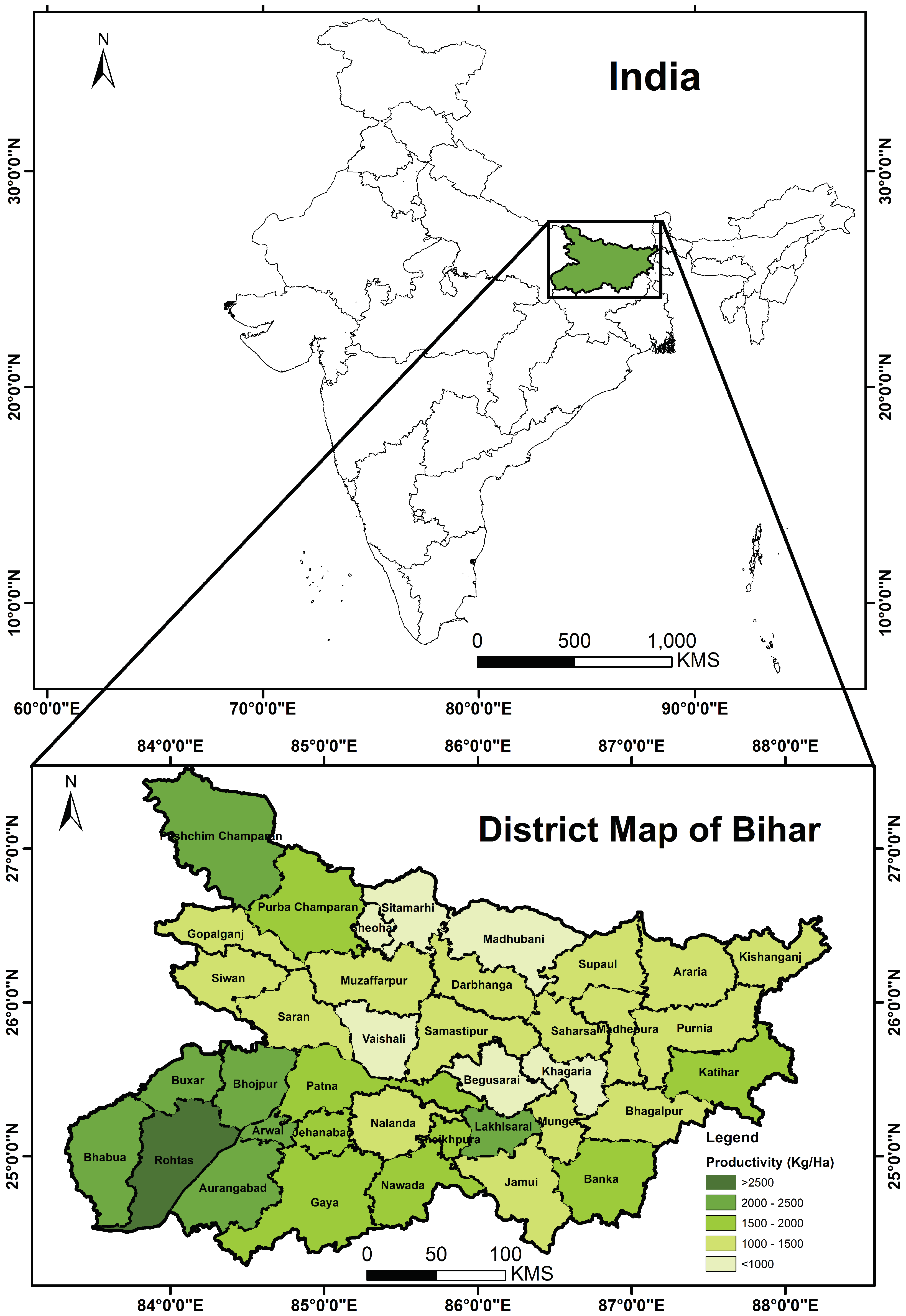
Figure 1. District-wise locational map of Bihar in India with the spatial distribution of District-Wise average rice productivity from 1991–1992 to 2014–2015 in kilogram per hectare in low to the high tone of green color. The dotted line within the solid boundary shows the administrative boundary of each district. (Figure was created using a licensed software ArcGIS version 10.2.1).
Sustainability 12 07023 g001
Figure 2. (a) Pearson’s Product Moment Correlation (PPMC) for the whole period (1991–1992 to 2014–2015) of rice productivity with climate indices in different seasons. Y-axis shows the value of PPMC. MI is for JJA season only therefore shown with the orange color bar. (b) Time series of rice productivity in Bihar. (c) The anomaly of Rice productivity in gray bars. Red (Black) numbers in the figure show the percent decline (increase) in Rice productivity. All the climate indices are multiplied by 15 to get standardized climate indices with rice productivity within the same figure. For rice productivity, Y-axis shows the anomalous percentage deviation and climate indices in degree celsius. Anomalous percentage deviated is calculated by subtracting the observed value of rice production from the five-year running mean of rice productivity.
Sustainability 12 07023 g002
Figure 3. Rainfall anomaly for the July-August-September (JAS) period of all the years with severer than −10% anomalous percentage deviation of rice productivity. The unit of rainfall anomaly is centimeter. Numbers within the map frame show the anomalous rainfall value and the regular black solid line is the district map of Bihar. (Figure was created using a free software GrADS version 2.0.2 (http://cola.gmu.edu/grads/downloads.php).
Sustainability 12 07023 g003
Figure 4. Anomalous soil moisture for JAS period of all the years with severer than −10% anomalous percentage deviation of rice productivity. Numbers within the map frame shows the anomalous soil moisture value and the regular black solid line is the district map of Bihar. (Figure was created using a free software GrADS version 2.0.2 (http://cola.gmu.edu/grads/downloads.php).
Sustainability 12 07023 g004
Figure 5. The composite map has a mean sum of anomalies of rainfall and soil moisture for events with severer than −10% anomalous percentage deviation in rice productivity. Map (a) is a composite of rainfall anomaly in JAS season, (b) represents composite soil moisture in JAS season, (c) is for composite soil moisture in the November-December-January (NDJ) season and (d) follows composite soil moisture in the March-April-May (MAM) season. Values above 95% significance level (green contours) from a two-tailed Student’s t-test are shown. The unit of anomalies of rainfall is centimeter. (Figure was created using a free software GrADS version 2.0.2 (http://cola.gmu.edu/grads/downloads.php).
Sustainability 12 07023 g005
Figure 6. Anomalous soil moisture for NDJ period of all the years with severer than −10% anomalous percentage deviation of rice productivity. Numbers within the map frame shows the anomalous soil moisture value and the regular black solid line is the district map of Bihar. (Figure was created using a free software GrADS version 2.0.2 (http://cola.gmu.edu/grads/downloads.php).
Sustainability 12 07023 g006
Figure 7. Anomalous soil moisture for MAM period of all the years with severer than −10% anomalous percentage deviation of rice productivity. Numbers within the map frame shows the anomalous soil moisture value and the regular black solid line is the district map of Bihar. (Figure was created using a free software GrADS version 2.0.2 (http://cola.gmu.edu/grads/downloads.php).
Sustainability 12 07023 g007
Figure 8. Composite temperature anomaly map for all the events with severer than −10% anomalous percentage deviation in rice productivity. (a,c) shows maximum temperature anomaly. (d,f) is for mean temperature anomaly, (g,i) is for minimum temperature anomaly. (a,d,g) represents JAS season of their temperature variants. (b,e,h) are for NDJ season their temperature variants. (c,f,i) show MAM season of their variants. Values above 95% significance level (green contours) from a two-tailed Student’s t-test are shown. The temperature unit is in degrees Celsius. (Figure was created using a free software GrADS version 2.0.2 (http://cola.gmu.edu/grads/downloads.php).
Sustainability 12 07023 g008
Figure 9. The composite map of anomalous SST (in °C), outgoing longwave radiation (in W/m2) and zonal wind (in ms−1) from NDJ to JJA seasons for all the events (as per Table 1). Blue to red shading in this map represents low to the high intensity of the anomalous sea surface temperature. Y-axis shows the latitude and the X-axis is for longitude. Values above 95% significance (green contours) level for SST from a two-tailed Student’s t-test are shown. Blue contours represent the anomaly of OLR. (Figure was created using a free software GrADS version 2.0.2 (http://cola.gmu.edu/grads/downloads.php).
Sustainability 12 07023 g009
Figure 10. Association of anomalous temperature (maximum and mean) and rainfall with productivity in Bihar for the period 1991–1992 to 2014–2015. Unit of productivity shown in the figure is percentage deviation based on the calculation as shown in Figure 2c, temperature anomaly is in °C and rainfall anomaly is in centimeter.
Sustainability 12 07023 g010
Table 1. Events of severer than −10% anomalous percentage deviation in different climatic phases. Prevailing phases of the three important climate indices during the event year is extracted on the basis of their significance at 90% level and >0.5 and <−0.5 value of Partial Correlation for the event years (Table S4). The value within brackets represent the year.
YearAnomalous Percentage DeviatedClimatic Phase
ONINIÑO 3SOI
1991–1992−12.05MJJ(1991)-JAS(1991)+ve-MAM(1991)-JJA(1991)-ve
1992–1993−29.76ASO(1991)-JAS(1992)+veNDJ(1991)-AMJ(1992)+veMAM(1992)-JJA(1992)-ve
2004–2005−35.3JJA(2004)-JAS(2004)+ve-MAM(2004)-JJA(2004)-ve
2005–2006−10.03ASO(2005)-JAS(2005)+veNDJ(2004)-DJF(2005)+veMAM(2005)-JJA(2005)-ve
2009–2010−23.51JJA(2009)-JAS(2009)+ve-MAM(2009)-JJA(2009)-ve
After Effects of Flood Occurrence in 2008
2010–2011−38.52JJA(2010)-JAS(2010)+veNDJ(2009)-FMA(2010)+ve-
Table 2. Mann Kendall Test trend and Sen’s Slope results of climatic variables for the period 1991–1992 to 2014–2015.
Variablez ValueSen’s Slopep-Value
Rainfall−1.611−1.9540.107
Temperature
(Max.)
3.480.040.0005
Temperature
(Mean)
4.0870.0350.00004
Temperature
(Min.)
3.340.0350.00084