Modelling Welfare Transitions to Prioritise Sustainable Development Interventions in Coastal Kenya

Abstract

Welfare transitions are weakly understood in sub-Saharan Africa due to limited panel data to analyze trajectories of household escaping from, falling into, or remaining out of deprivation. We model data from 3500 households in coastal Kenya in three panels from 2014 to 2016 to evaluate determinants of welfare by multidimensional and subjective measures. Findings indicate that more than half of the households are deprived, with female-headed households being the most vulnerable and making the least progress. The subjective welfare measure identified three times more chronically poor households than the multidimensional metric (27% vs. 9%); in contrast, the multidimensional metric estimated twice as many ‘never poor’ households than the subjective measure (39% vs. 16%). The ‘churning poor’ were broadly consistent for both measures at roughly half the sample. Four welfare priorities converged from modelling welfare transitions. Broadening access to secondary education and energy services, improving the reliability and proximity of drinking water services, and ending open defecation improve welfare outcomes. While the policy implications do not align neatly with Kenya’s national and county government mandates, we argue that prioritising fewer but targeted sustainable development goals may improve accountability, feasibility, and responsibility in delivery if informed by local priorities and political salience.

1. Introduction

The nature of welfare in rural Africa is often characterized by lack of or poor access to public services such as water, education, health, energy, and transportation, among others [1,2,3,4]. While the effects of these factors vary between different groups of households or individuals in both space and time, their empirical relationships to welfare are often not properly understood due to limited data availability. The existing information asymmetry in rural Africa limits objective assessments, as baseline conditions for social, economic, and environmental systems are commonly absent, unavailable, or incomplete to support empirical analysis of the relationships between welfare and its determinants. Distributional implications and impacts for local populations over time and across varying environmental conditions are poorly documented, providing a weak platform to inform policy and practice to guide sustainable development pathways. Modelling welfare transitions will contribute to understanding the links between welfare and the determinants of welfare to inform policy priorities in the context of varying economic, environmental, or political shocks. This study employs longitudinal data to model multidimensional and subjective welfare transitions and their determinants to accelerate sustainable development goals in rural Kenya.

Africa’s development pathways in poverty reduction will increasingly be shaped by identifying more effective and equitable policy and practice to balance competing goals of economic growth and environmental sustainability [5,6,7,8]. While the sustainable development goals provide some of the development pathways through 17 goals, 169 targets, and 230 indicators [9], there remains a challenge for most developing countries to balance and prioritise the multiple and overlapping goals given the rapidly changing environmental, economic, and political constraints. Progress towards poverty reduction has been characterised by varying degrees of success and failures from one country to another. With the Millennium Development Goals reporting substantial global progress in halving the number of people living below the poverty line of USD 1.25 a day [10,11], findings in rural Africa show that there were 50 million more people in 2012 than in 1990 living below the poverty line [12]. Lessons from the uneven and unsatisfactory progress in the Millennium Development Goals promote a more pragmatic set of goals which meet social priorities to offer a cost-efficient, welfare-enhancing, and politically-appropriate approach.

Poverty is a condition of multiple deprivations for different individuals or households and the vulnerable, and it also varies substantially between countries and over time [13,14]. The dynamic nature of poverty requires a clear metric and measurement approach to ensure policies are effective and address the needs of the poor. Common approaches to measuring poverty in literature include income poverty, consumption poverty, multidimensional welfare, and subjective welfare [13,15,16,17,18,19,20]. Poverty and welfare differ in the measurement approach with diverging implications on policy and practice. While poverty metrics are mostly generated from income and expenditure data, welfare measurements recognise health, education, assets, and some social deprivations. Several studies have tested and used assets, health, education, and social deprivations to construct welfare metrics, and these welfare measurements are increasingly being used to assess trends in economic development and ranking countries over time [21,22]. The indicators used in these studies range from household assets such as livestock, bicycles, radios, electricity, etc., to sources of water supply, sanitation variables, and type of housing structures such as wall, floor, and roof materials, and other social measures including health, education, transport, etc. [21,23,24]. This approach is an attempt to shift away from income and expenditure data that is rarely available in developing countries, making it difficult to estimate wealth effects. This paper focuses on these welfare measures with the poor and non-poor being described by low welfare and high welfare statuses, respectively.

There is a growing interest in subjective welfare measures [25,26] with studies exploring the possibility of such a metric to converge with multidimensional welfare measurements [27,28]. While subjective welfare measurements prioritise self-assessments of an individual or household’s welfare, they are not perfect and may suffer from limitations relating to bias from cognition, representation, and stability [29]. Cognition bias relates to the interpretation of the questions on welfare status in a consistent and equivalent manner. It is related to what Beegle et al. [28], term as frame of reference, where individuals self-evaluate themselves in reference to their neighbors. For instance, poor households will tend to have a limited understanding of being well-off if the majority of the neighbors are poor, while a wealthy household is likely to be more exposed with broader experiences of life and will have a different understanding of being well-off. This may affect the consistency of the subjective measure. Helliwell et al. [30], suggest that complete faith in subjective welfare assessments would be a bold and probably unsubstantiated claim, but the alternative of externally deciding what matters to people most is equally fraught. Representation also matters in subjective measures in relation to whom the respondent can reasonably and accurately answer for. This is important as multidimensional welfare measures rely on commonly owned assets and other household characteristics. This has implications on the stability of welfare measurements over time demanding the need for consistency in data collection to monitor and evaluate progress while ensuring poverty reduction interventions reflect the needs of different groups.

Robust and replicable welfare metrics are pertinent to assessing welfare transitions to categorise different groups of households, such as those churning in and out of poverty, those that are chronically poor, and those that are never poor [31,32]. These categories enable a wider and deeper understanding of welfare and may further be disaggregated by sex of household head. Studies show that chronic poverty is disproportionately common among historically marginalized groups such as women, making it harder for female-headed households to escape poverty [33]. Gender discrimination on the other hand exacerbates inequality in employment and wage compensation, land ownership, and inheritance rights, social exclusion in economic and political institutions increasing their vulnerability to chronic poverty [34]. Further evidence in literature show that female-headed households are more likely to fall into poverty or remain poor compared to male-headed households [12,35,36]. This however varies from country to country, and is largely a function of availability or lack of policies that directly or indirectly discriminate against women. For example, some studies have found that female-headed households tend to perform better in resource mobilisation and management than male-headed households with implications on poverty transitions if the policy framework provides a conducive environment for growth and development [37]. Thus, it is important to ascertain the vulnerability of female-headed households as it might be an exception and not the norm in some places. Policy and practice need to accommodate the needs of different groups in different levels of welfare and vulnerabilities.

Delivery of policy remains a core mandate of governments and their relevant departments and institutions. Where a working form of governance exists with checks and balances, bilateral donor support and institutions mandated to address poverty reduction may accelerate attainment of the sustainable development goals. Kenya is a good example, where decentralization of the central government led to formation of 47 county governments with replicated institutions and ministries in each county to offer services and bring resources closer to the people [38,39]. Kenya remains on a trajectory of positive growth under this new form of governance if coherent legal and policy frameworks are strengthened at the county level [38,40]. The paper models determinants and transitions of welfare to inform and guide policy priorities and practice in coastal Kenya, drawing from 3500 longitudinal household surveys over three waves (three separate surveys conducted annually using the same questionnaire) of data to (a) understand determinants of welfare by location and over time, (b) measure welfare, (c) evaluate welfare transitions, and (d) identify policy action to improve welfare. The next section describes the data and methodology used to assess multidimensional and subjective welfare, subjective welfare and modelling random effects of different determinants on welfare. We then report the results by different profiles of poor (low welfare) and non-poor (high welfare) categories as well as sex of household head. Section 4 discusses the results and Section 5 concludes.

2. Methodology

2.1. Study Site and Sampling Frame

The study site is Kwale County, Kenya, south of Mombasa and adjacent to northern Tanzania (Figure 1). The study area covers 2156 km² in Lunga Lunga, Msambweni, and Matuga sub-counties with around 300,000 residents [41]. The study area’s climate has a bi-modal rainfall pattern with an average annual precipitation of approximately 1380 mm, but with significant inter-annual and spatial variability. The coastal lowland of the study area is the wettest, with the climate getting drier to the west and north. The average annual temperatures are above 28 °C [42]. About 90 percent of the population lives in rural areas, with 7 out of 10 people living below the poverty line of less than USD $1.25 a day, and this headcount ratio has remained notoriously high over the last decade [43,44]. Since 2013, the pace of environmental, economic, social, and political change has increased with the establishment of two new and major economic activities in the area. Kwale International Sugarcane Company Limited (KISCOL) has been progressively rehabilitating 5500 hectares of sub-surface irrigated sugarcane, including the commissioning of its own sugar mill in 2015. Adjacent to the sugarcane plantations is the country’s newest and largest mining operation (Kwale Mineral Sands Project). The mine, operated by Base Titanium Ltd., is currently projected to export 6.5 million tonnes of titanium ore by 2028 from Likoni port, some 30 km north of the mine site. Scattered around the mine site and sugarcane plantation are around 300 functional handpumps (5–30 m deep) providing drinking water to communities, schools, dispensaries, and health centres.

In August 2013, a water point survey identified 574 handpumps (all Afridevs) of which 45% were non-functioning—at the time, this represented the known population of handpumps traced in the area. It captured technical, institutional, operational, financial, and geographical information through structured interviews with waterpoint users [45]. GSM-enabled transmitters were installed on 300 operational handpumps to transmit and record daily pumping to estimate water usage and functionality [46,47]. At the time of the water point survey, no other formal infrastructure such as small piped schemes, kiosks, or solar pumps were identified. The villages in the study area depended on these handpumps as the main improved drinking water sources [48]. A sample of 571 handpump locations was used as a sampling frame for the longitudinal household survey. A pilot survey was conducted with 19 enumerators recruited from communities across the study area who administered the survey in local languages (Swahili, 53.8%; Digo, 42.6%; Duruma, 2.1%; other, 1.5%). The main survey entailed a range of themes including demographic, socio-economic status of household (here including livelihood, concerns, and subjective welfare), household health status, water sources, water point management, water payments, water resources management, governance, and political engagement [49]. From 571 handpumps, a stratified random sample of households was produced, yielding on average 3500 survey participants. An average of six households were randomly selected at each handpump, both functional (n = 314) and non-functional (n = 257) during the household survey: At each handpump, a member of the Water User Committee was selected to draw a map of all the households using that particular waterpoint and number them. Through the use of a random number generator, six households were selected. If no one was available at the selected household, the enumerators interviewed the nearest available household. Oral informed consent was obtained from all participants. Three household surveys were conducted in October 2013 to January 2014, March to May 2015, and September to November 2016. The same respondents were interviewed each round using the same questionnaire. This resulted in three waves of longitudinal (panel) data. The attrition rate was 3% (roughly 100 households) in the second and third wave due to households moving away or respondents refusing to be re-interviewed. The total sample size used in the analysis after data cleaning was 3234 households. All the households surveyed were geo-referenced for mapping purposes.

Ethical permission to conduct this survey was provided by the University of Oxford’s Central University Research Ethics Committee and research permission granted by the Government of Kenya’s National Council of Science and Technology, Kenya (NCST/RCD/17/013/132, September 2013). All interviews were voluntary with informed consent procedures observed in the local language. Data have been anonymised and stored in encrypted files.

2.2. Measuring Welfare and Transitions

A multidimensional asset-based welfare index was constructed using 29 indicators drawn from household characteristics, dwelling characteristics (including type of roof of housing, walls, and flooring material), assets, and consumables [49]. These indicators were combined together using weights. The weights used to compute the welfare index were generated from principal component analysis, an approach used repeatedly in literature to estimate welfare indexes [21,23,50,51]. Principal component analysis is mainly used for dimensionality reduction of continuous variables, but has been used on binary variables, not for dimensionality reduction, but to use the eigenvectors from the co-variance matrix to decide on weighting the variables. The index generated is easy to defend empirically and has been observed to be internally and externally coherent [21]. This methodology broadly follows the Kenya Demographic and Health Survey and the Kenya Integrated Household Budget Surveys methodology in assessment of welfare in Kenya [44,52].

Households were assigned a score of ‘1′ if they met the criteria for an indicator, otherwise ‘0′. Households with missing data on at least one of the indicators were removed from the analysis. We then developed a multidimensional welfare index for the year 2014 based on all indicators. This was done for years 2014 and 2015 using the same weights generated by the PCA with 2014 as the reference year. Applying different weights for the year 2015 would have made the two years incomparable. The computed welfare index was normalised between 0 and 1, where households scoring higher values were relatively well-off compared to those scoring values close to zero. To compare the fraction of households across different welfare groups, we split the welfare index range into five wealth groups with equal range defined by the lowest welfare group with a welfare index ranging between 0 and 0.2, while the highest wealth group had a welfare index of more than 0.8. We refer to these as welfare quintiles and compute the fraction of households in each welfare quintile [49].

The welfare index generated values from zero to one with welfare quintiles derived from this range with households located by their value in the range. As such, the share of households by welfare quintile is not even, but reflects the relative distribution across the welfare scale which permits assessment of welfare movements over time. Filmer and Pritchett [21], used three cut off points to categorise households into poor, middle, and the richest (i.e 0.4, 0.8, and above 0.8, respectively). In this paper, the interest was to estimate two binary groups, poor and non-poor, for the purpose of assessing the transitions. We thus collapsed the middle wealth group and the richest group (as defined by Filmer and Pritchett) into the non-poor category and maintained the poor group. For the households that fell into the bottom 2 welfare quintiles (welfare index less than 0.40), we categorised them as poor, while those that were in the top three welfare quintiles (welfare index equal to 0.40 or greater) were categorised as non-poor. We defined female-headed households as households with only female adults (above 15 years old), and male-headed households as households with at least a male adult. To understand the dynamics of households moving in and out of poverty, we applied a one-way tabulation of the poor and non-poor households and further computed the transition probabilities of either a household remaining poor or transiting to a non-poor state [32].

To explore welfare heterogeneity across different geographies, we categorized the households into three groups by a simplified typology of three economic geographies in the study area: (1) The south-eastern coastal belt with people living within a 5 km strip of the sea (50.6% of the sample), whose main economic activity is fishing; (2) inland and more remote areas south and south-west of the Shimba Hills and away from the coastal margin (39.1% of the sample), where the main economic activity is farming; and (3) the small town of Ukunda/Diani, which largely serves the tourism industry along Diani beach (10.3% of the sample), see

Table 1. Summary statistics of variables by sex of household head (n = 3234).

		Households with Only Female Adults, n = 526 Mean			Households with at Least One Male Adult, n = 2708 Mean
	Variables	Wave 1	Wave 2	Wave 3	Wave 1	Wave 2	Wave 3
Geographical Location *	Coastal	0.50	0.50	0.50	0.50	0.50	0.50
	Inland	0.45	0.45	0.45	0.38	0.38	0.38
	Ukunda	0.07	0.07	0.07	0.12	0.12	0.12
Water Services	Affordable	0.10	0.07	0.05	0.13	0.08	0.05
	Close (distance to water source)	0.59	0.60	0.58	0.57	0.63	0.61
	Reliable	0.30	0.25	0.21	0.31	0.29	0.22
	Only source	0.27	0.21	0.20	0.25	0.22	0.22
Water Infrastructure	Handpump	0.67	0.66	0.62	0.64	0.66	0.60
	Piped	0.11	0.14	0.19	0.17	0.17	0.23
	Unprotected well	0.11	0.14	0.15	0.11	0.11	0.12
Highest Education Attained	Primary	0.61	0.68	0.61	0.53	0.49	0.50
	Post Primary	0.02	0.01	0.01	0.02	0.02	0.03
	Secondary	0.27	0.18	0.24	0.35	0.37	0.36
	College	0.03	0.03	0.04	0.06	0.08	0.06
	University	0.02	0.01	0.03	0.02	0.03	0.03
Energy	Electricity (national grid)	0.04	0.04	0.09	0.08	0.09	0.18
	Solar panel	0.02	0.04	0.12	0.05	0.08	0.13
Agriculture	Own Livestock	0.21	0.11	0.41	0.21	0.22	0.49
	Own >2 acres land	0.44	0.44	0.65	0.43	0.49	0.63
Sanitation	Open defection	0.53	0.44	0.36	0.43	0.38	0.28
	Cases of diarrhoea in last two weeks	0.10	0.10	0.07	0.08	0.10	0.06
Multidimensional Welfare	Poor (bottom 40%)	0.53	0.41	0.33	0.43	0.31	0.24
Subjective Well Being
	Poor (not well-off)	0.62	0.70	0.59	0.56	0.59	0.48

Standard deviations not shown since the variables are binary. * The totals may not add up to 100% due to rounding.

.

2.3. Measuring Determinants of Welfare

To assess the determinants of welfare, we considered an analytical approach that applies the random effects model to both a multidimensional welfare index and a subjective welfare index. The subjective welfare index is derived from three categories asked to each household, i.e., ‘not well-off’, ‘average’, and ‘well-off’. A small fraction of households (less than 0.5%) identified themselves as well-off, and this category was excluded from the analysis. The remaining two categories were classified into poor (for households categorising themselves as not well-off) and non-poor (for households categorising themselves as average). The independent variables considered in the analysis include water services (by stated concerns with affordability and reliability, distance and dependence on only one source), type of water infrastructure, geographical location, level of education by household measure, access to energy, agriculture (land ownership and livestock), and sanitation and health (type of latrine and two-week diarrhoea recall).

Our analytical strategy was to use the three waves of longitudinal data to model the effects of independent variables on welfare while controlling for social, environmental, or political heterogeneity [53]. There are a range of models that can be used in longitudinal data techniques, and each model is employed based on a set of conditions. The two common longitudinal data models (in the case of a continuous dependent variable) are the fixed effects model and the random effects model. A fixed effects model is commonly used where the individual specific effects (unobserved heterogeneity across individuals) are correlated with the regressors (independent variables), while a random effects model is used where the individual effects are not correlated with the regressors but rather assumed to be randomly distributed over time [53]. The fixed effects model estimates these individual specific estimates using dummy variables with the regressors being considered time-variant. However, in situations where the regressors are time-invariant, the random effects model is more applicable.

While making inferences as to which of the two models to use, some researchers advise using certain statistical tests of endogeneity such as the Hausman–Taylor test [54,55], a standpoint which is strongly contested on grounds that it tends to over reject the null hypothesis. Other studies suggest an alternative decision-making process, which we considered in this study, based on the factors described by Borenstein et al. [56]. This approach helped to decide on which model fit the distribution of effect sizes and takes account of the relevant error sources, based on the nature of the data at hand, the process of data collection, whether all the waves shared a common effect size, and the research questions of interest [57], which we discuss below.

There are at least three considerations which emerge from the longitudinal design, i.e., common effect size across the sample, variability within the subjects, and effects of time-invariant variables in the study. First, not all individuals were interviewed by the same enumerator in every wave (year), and the three studies included in this analysis were not strictly identical. The first study was, for example, conducted in the dry season, the second one was conducted during the wet season, and the third was conducted in a year that the country experienced one of the worst droughts in history. This introduced randomness in the survey administration with implications on functional similarity of each survey. The assumption that there was a common effect size across the wider sample was thus questionable, making a random effects model more justifiable [56,57]. Second, the amount of variability within subjects was considered to be small for a fixed effects model to be consistent and efficient. Third, while some of the independent variables were time-invariant, the time-variant ones did not change substantially every year, as shown in Table 1. The key insight being that if the unobserved variable does not significantly change over time, they will be fully subsumed in a fixed effects mode and any remaining within household variations may be due to changes of other observable variables over time [58]. In a random effects model, we assume that the unobserved variables are uncorrelated with the observed variable. While we recognize this assumption may be weak, the alternative model, fixed effects, often results with very high standard errors if the assumption holds true. In addition, estimating the effects of time-invariant variables, specifically female-headed households, was of interest to this study. Employing a fixed effects model would have dropped them out of the analysis, the random effects model on the other hand allows for estimation of effect for time-invariant variables and remained desirable in this case [58]. With these considerations, we employed the random effects model with the welfare index as the dependent variable.

While a random effects model was considered effective in this study, we recognise the limitations of the model with possible biases due to the omitted variable problem [53]. The independent variables considered in this study do not account for all the possible covariates of poverty. Some of the omitted variables include, for example, household size, age, or employment, which happen to be exogenous variables, and therefore may introduce some bias in the analysis. Controlling for the omitted variable problem was a challenge due to the cultural context, for example, household size was difficult to ascertain in every wave, and it was complicated by seasonal migration and the challenge of establishing the size in terms of daily living or broader economic welfare. Employment variable was equally complex with households living in extended families where the wage earner is never the same person every time. Adding the household size and age variables in the model showed that they were both statistically insignificant (p > 0.01) in the random effects model (except household size was significant in the fixed effects model) with almost zero effect on the dependent variable. Results showing these data are appended in the Supplementary Materials, and we discuss the other factors here in the paper.

The statistical test for endogeneity, Hausman test, between fixed effects and random effects models was equally done for completeness [54,55]. We note that the deductions from the output of the fixed effects model were similar to those of the random effects model in terms of statistical significance and direction of influence on the dependent variable, leading to similar conclusions. Results for both the Hausman test and the models are appended in Supplementary Materials.

In the case of binary dependent variables, the commonly used models are probit and logit models. The fundamental differences between probit and logit models is that probit models use the cumulative distribution function of the standard normal distribution while the logit (logistic) model uses the cumulative distribution function of the logistic distribution [53,59]. However, both models are based on probability distributions and yield similar results [60]. The logit model coefficients can be interpreted as odds ratios, making it more desirable in this analysis. Given that the subjective welfare measure was binary (in this case well-off and not well-off categories) and longitudinal, the random effects logit model was used. This was necessary to compare the outcomes of both the welfare index and the subjective welfare assessment in assessing the effects of the different independent variables on welfare.

We further note that the resulting outputs from the modelling only supports correlation between the depended variable and the independent variables. We cannot claim causality here as the study was not a randomized control trial. While it might be remotely possible to assess for causation from longitudinal studies, the study design and data available in this research was not sufficient to support any causality analyses or claims.

3. Results

We report the descriptive findings which reveals the nature of welfare transitions (Table 1). First, welfare is generally improving, though less so for female-headed households. Second, welfare transitions identify a substantial number of households that are churning poor and chronically poor with implications to design of policy and practice. Third, subjective welfare is less optimistic than the multidimensional index. Fourth, four policy interventions are identified that reflect the needs of the people to accelerate sustainable growth and development.

3.1. Welfare by Household Categories

Households with only female adults (female-headed households) accounted for 16 percent of the total sample size with the remainder being male-headed households. About a half of both female and male-headed households reside on the coastal region, less than 10 percent reside in the more urban area of Ukunda, while the rest were observed to reside in the Inland regions. In terms of water services for female-headed households, we saw a reduction in the fraction of households with access to affordable and reliable water services over time. Households with affordable water services (one in ten in wave 1) decreased by half over the three years, while those with reliable water services decreased by 9 percent. While distance to water sources remained more or less the same in all the years, households with alternative water sources increased from 73 percent to 80 percent over the three years. Similar changes across the years were observed with male-headed households.

Water supply for the majority of households is from handpumps, though there is an almost doubling in growth of access to piped systems over the period. Household water supply is considered ‘close’ by most respondents, with reliability decreasing over time and affordability a concern for almost all households (95%). The most common water infrastructure for over two thirds of all the households was handpumps. While dependence on handpumps was observed to decrease by four to five percent between wave one and wave three for all the households, dependence on piped water systems increased by six percent for male-headed households and eight percent for female-headed households.

In terms of access to education, about one in two male-headed households had household members who had attained or were still in primary education level. About 36 percent of male-headed households had household members who had attained or were still in secondary education level at any point in time over the three waves. Female-headed households were 1.2 times more likely to have household members with or who have had access to primary education compared to male-headed households. However, female-headed households were about 1.6 times less likely to have household members transiting to secondary schools compared to male-headed households. Households with at least a male adult were 1.5 times more likely to have children in secondary schools and two times more likely to have children in college or university compared to female-headed households.

Access to national grid electricity connection remained low in wave two for female and male-headed households at four and eight percent, respectively, compared to the national average of 41 percent. Similarly, access to solar panels was low for female and male-headed households compared to the national average of 14 percent [44]. While the overall access to energy was low, we observed a two-fold increase in access to electricity from the national grid for both female and male-headed households between wave one and wave three. Similarly, access to solar panels increased six-fold for female-headed households and two-fold for male headed households between wave one and wave three.

Livestock ownership rates for female and male-headed livestock in wave one was similar, however, in wave two, female-headed households who owned livestock decreased by half compared to the male-headed households. In addition, the livestock ownership rates for both female and male-headed households were observed to increase three-fold from wave one to wave three. These substantial changes in livestock ownership from year to year made limited sense and requires further analysis and caution in interpretation. Land ownership, on the other hand, appeared stable across wave one and wave two. In wave three, land ownership increased by approximately 20 percent for both female and male-headed households. There were more male-headed households who owned land of more than two acres compared to female-headed households, at any point in time.

In terms of sanitation, open defecation rates among female-headed households were slightly higher than among male-headed households. More than one in two female-headed households were reported to lack any kind of sanitation facility (toilet) in wave one. Open defecation rates were observed to decrease in wave two and three by about 17 percent points. Male-headed households were 1.2 times less likely to lack any form of toilet compared to female-headed households. However, the open defecation rates among male-headed households were equally high by standards, although the rates declined over time by close to 15 percent points. While diarrhoea cases in the last two weeks for all children under 15 years (based on recall) were observed in less than ten percent of all the households, they were slightly more common among female-headed households than male-headed households across all the waves.

The multidimensional welfare index was able to classify the poor and non-poor households, also based on sex of household head. Results showed that the number of poor female and male-headed households decreased by 20 percent points between wave one and wave three. However, the likelihood of female-headed households to be poor compared to male-headed households was observed to increase from 1.2 in wave one to 1.4 in wave three. The subjective welfare index on the other hand classified three out of five female-headed households as poor in wave one and wave three, and it also classified two thirds of female-headed households as poor in wave two. Overall, female-headed households were observed to be more likely to subjectively identify themselves as poor compared to male-headed households, especially in wave three.

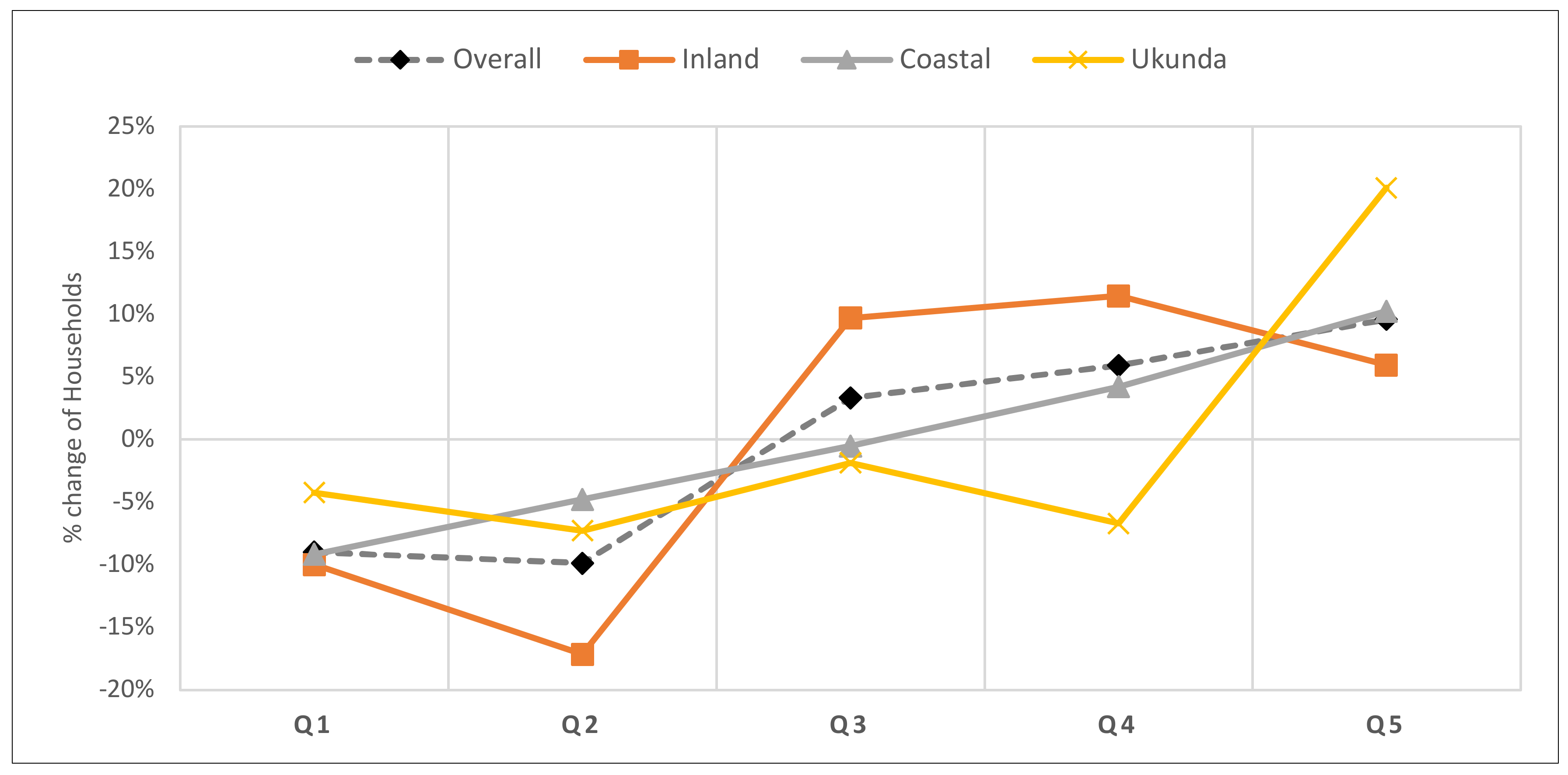
3.2. Welfare Transitions

Table 2. (a). Welfare transitions by multidimensional and subjective measures (2014–2016) (n = 3234). (b). Subjective welfare transitions for 2014, 2015, and 2016 (n = 3234).

(a)
	Overall		Between		Within	Welfare Transitions
multidimensional Welfare	Freq.	Percent	Freq.	Percent	Percent	multidimensional Welfare	Non-poor	Poor
Non-poor	6405	66	2932	91	73	Non-poor	81% (76%)	19% (24%)
Poor	3297	34	1980	61	56	Poor	55% (49%)	45% (51%)
Total	9702	100	4912	152	66	Total	71% (63%)	29% (37%)
(b)
	Overall		Between		Within		Subjective Welfare Transitions
Subjective Welfare	Freq.	Percent	Freq.	Percent	Percent	Subjective Welfare	Non-poor	Poor
Non-poor (Average)	4238	44	2356	73	60	Non-poor (Average)	59% (51%)	41% (49%)
Poor (not well-off)	5455	56	2714	84	67	Poor (not well-off)	34% (27%)	66% (73%)
Total	9693	100	5070	157	64	Total	44% (35%)	56% (65%)

NB: Numbers in brackets are for female-headed households. The totals may not add up to 100% due to rounding.

summarises welfare transitions by the multidimensional index and the subjective assessment. They are reported by a one-way tabulation of welfare decomposed by counts between and within components in longitudinal data. A summary of transition probabilities of changes in multidimensional welfare and subjective welfare over time. The overall column of Table 2a shows that we had 6405 household-cases of data (64 per cent) where the household was non-poor, and 3297 household-cases (34 per cent) where they were poor. The between column shows the total count of households that have been, at least on one occasion over the three waves, poor or non-poor. There were 1980 households that have been poor, while 2932 households have never been poor on any one occasion. This makes a total of 4912 households having been either poor or non-poor on any one occasion across the three waves. This contrasts with a total sample size of 3234 households, meaning that some households have been poor in one occasion and non-poor at other times (churning in and out of poverty). The within percent tells us the fraction of the time a household has been poor or non-poor. Looking at the first row, conditional on a household ever being non-poor, 73 percent of the time that household is non-poor while conditional on a household ever being poor (second row), 56 percent of the time that household is poor. This is a measure of the stability of households meaning that the non-poor households tend to be more stable than poor households. The overall stability of the households being poor or non-poor, normalized between the weighted average of the within percent, was measured at 66 percent.

The welfare transitions summary in Table 2a shows that in each period, about 81 percent of those households who were initially non-poor remained non-poor in the next period, whereas about 45 percent of those who were initially poor remained poor in the next year. Although non-poor households had a 19 percent chance of becoming poor the next year, poor households had a 55 percent chance of becoming non-poor. Female-headed households who were initially non-poor had a 24 percent chance of becoming poor the next year, while those who were initially poor had a 49 percent chance of becoming non-poor. Around one in two female-headed households of those who were poor remained poor every year, while 76 percent of those who were non-poor remained non-poor every year.

The subjective welfare tabulation in Table 2b reported fewer household-cases categorizing themselves as non-poor, 4238, in comparison to the welfare index which had 6405, and the poor category reporting an overall 5455 household-cases in more than half of the data. The between summary reports a total of 2356 households that have ever been non-poor (subjectively) on any one occasion, with another 2714 households that have ever been poor on any one occasion. Again, this makes a total number of households greater than the actual sample size, meaning some households have been in one category more than once over the three waves. This is further elaborated in

Table 3. Multidimensional and subjective welfare transitions by chronic, churning, and never poor categories.

Wave 1	Wave 2	Wave 3	Chronic Poor	Churning Poor	Never Poor
Poor (not-well-off)	Non-poor (Average)	Non-poor (Average)		17% (10%)
Poor (not-well-off)	Non-poor (Average)	Poor (not-well-off)		7% (7%)
Poor (not-well-off)	Poor (not-well-off)	Non-poor (Average)		11% (13%)
Poor (not-well-off)	Poor (not-well-off)	Poor (not-well-off)	9% (27%)
Non-poor (Average)	Non-poor (Average)	Poor (not-well-off)		5% (6%)
Non-poor (Average)	Poor (not-well-off)	Non-poor (Average)		8% (10%)
Non-poor (Average)	Poor (not-well-off)	Poor (not-well-off)		4% (10%)
Non-poor (Average)	Non-poor (Average)	Non-poor (Average)			39% (16%)
		Total	9% (27%)	52% (56%)	39% (16%)

NB: Text and numbers in brackets refer to subjective welfare measures.

.

The transitions based on the subjective welfare measure showed that over two thirds of the households initially in the poor category remained poor, while 59 percent of these households initially in the non-poor category remained non-poor the next year. Households initially in the non-poor category had a 41 percent chance of moving into the poor category, while those in the poor category had a 34 percent chance of moving in the non-poor category. Female-headed households that were initially non-poor had a 49 percent chance of becoming poor the next year, while those initially in the poor category had a 27 percent chance of becoming non-poor the next year.

To identify the pattern a household followed across the three waves, we use three categories similar in principle to the poverty tiers conceptualized by [32], i.e., those who are chronic poor, churning poor, and the never poor. In this case, a household that was never poor could follow the pattern ‘non-poor, non-poor, non-poor’ in all three waves based on the welfare index measure, or it could be average in all the three waves based on subjective welfare measure. The chronic poor could assume a pattern of poor, poor, poor. The churning poor are categorized as households who have been poor in at least one occasion over the three waves.

Looking at the patterns of welfare in Table 3 for all the households, we observed that about 39 percent of the households have never been poor, while about one in ten households have been chronically poor, and more than half of all the households have been churning poor. The subjective welfare measures identified fewer households being in the never poor category, 16 percent, and about three-times more households being in the chronic poor category in comparison to the multidimensional welfare index. Both welfare measures had similar fractions of households in the churning poor category.

Table 4. Multidimensional and subjective welfare transitions for chronic, churning, and never poor categories by sex of household head.

	Patterns		Households with Only Female Adults, n = 526			Households with at Least a Male Adult, n = 2708
Wave 1	Wave 2	Wave 3	Chronic Poor	Churning Poor	Never Poor	Chronic Poor	Churning Poor	Never Poor
Poor (not-well-off)	Non-poor (well-off)	Non-poor (well-off)		18% (12%)			17% (10%)
Poor (not-well-off)	Non-poor (well-off)	Poor (not-well-off)		8% (10%)			6% (10%)
Poor (not-well-off)	Poor (not-well-off)	Non-poor (well-off)		13% (5%)			11% (6%)
Poor (not-well-off)	Poor (not-well-off)	Poor (not-well-off)	14% (10%)			8% (17%)
Non-poor (well-off)	Non-poor (well-off)	Poor (not-well-off)		4% (12%)			5% (14%)
Non-poor (well-off)	Poor (not-well-off)	Non-poor (well-off)		7% (5%)			8% (7%)
Non-poor (well-off)	Poor (not-well-off)	Poor (not-well-off)		6% (8%)			4% (10%)
Non-poor (well-off)	Non-poor (well-off)	Non-poor (well-off)			29% (37%)			41% (25%)
		Total	14% (10%)	56% (52%)	29% (37%)	8% (17%)	51% (57%)	41% (25%)

NB: Text and numbers in brackets refer to subjective welfare measures.

disaggregates the data by sex of the household head. The multidimensional welfare index showed that female-headed households were 1.4 times less likely to be non-poor (never poor) and 1.8 times more likely to be chronic poor in all the three waves compared to male-headed households. In contrast, subjectively welfare measure showed that female-headed households were 1.4 times more likely to be non-poor and 1.7 times less likely to be chronic poor in all the three waves compared to male-headed households.

Overall, the subjective welfare and the multidimensional welfare index measures appeared to converge for the churning poor households. For all households, we observed that the subjective welfare measure grouped more households in the chronic poor category compared to the multidimensional welfare index, while in the never poor category the multidimensional welfare index identified more households compared to the subjective welfare measure, see Table 3. On the other hand, female-headed households’ subjective welfare measure converged closely to the multidimensional welfare index for both chronic, churning, and poor categories, however, it was observed to substantially diverge for male-headed households for the chronic poor and the never poor category, see Table 4.

To examine welfare transitions between the welfare quintiles by geographical location, we plotted the overall changes in the fraction of households in each welfare quintile between wave three and wave one, see Figure 2. Where the graph shows values close to zero means that there were no households transitioning in or out of that welfare quintile. A positive change depicts a household moving into that welfare quintile while a negative change depicts a household moving out of that welfare quintile. For the overall households, we observed at least 10 per cent of households transitioning from each of the two lower welfare quintiles, Q1 and Q2, to the higher welfare quintiles, indicating an overall improvement in welfare. The geographical location with the most improvement in welfare was the inland region where 10 per cent and 17 per cent of the households transitioned from Q1 and Q2, respectively, to higher welfare quintiles. While Ukunda region had the least fraction of households moving out of the bottom four welfare quintiles, the region saw a substantial increase in the fraction of households moving into the top most welfare quintile, Q5. The coastal region was the least improved in terms of welfare with fewer fractions of households transitioning from the lower welfare quintiles.

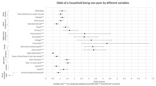
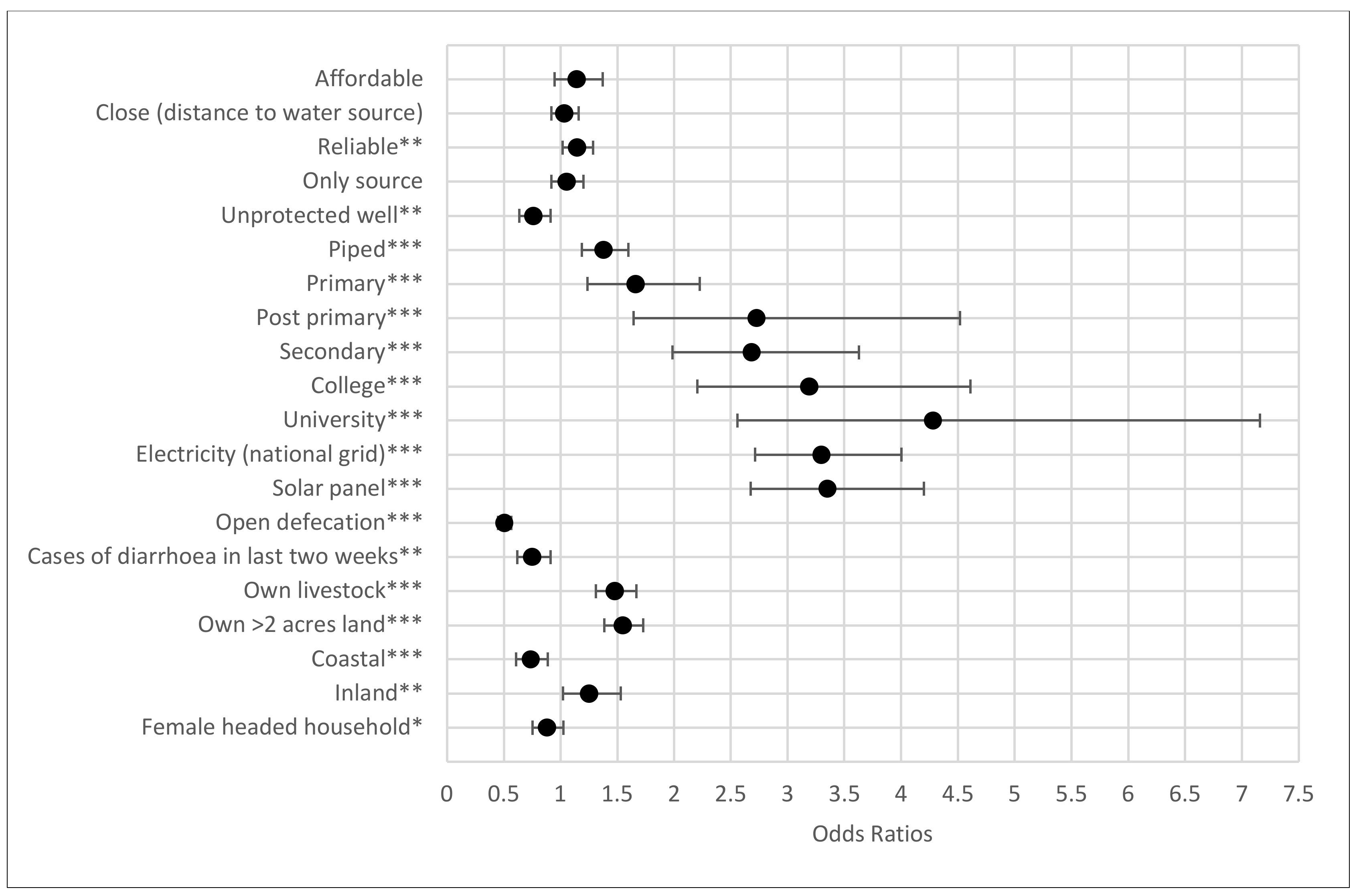
3.3. Random Effects Estimation with Welfare Measures

The longitudinal dataset made it possible to estimate the effects of the independent variables on both multidimensional welfare index and the subjective welfare measure across households and over time. The random effects model,

Table 5. Random effects coefficients for multidimensional welfare.

Category	Variables	Coef.	Std. Err.	z	[95% Conf. Interval]
Water Services	Affordable	0.01164	0.00845	1.38	−0.00493	0.02820
	Close (distance to water source)	0.03919 ***	0.00523	7.49	0.02894	0.04943
	Reliable	0.01671 ***	0.00525	3.18	0.00641	0.02700
	Only source	0.00797	0.00614	1.30	−0.00407	0.02000
Water Infrastructure	Unprotected well	−0.01357 *	0.00814	−1.67	−0.02953	0.00239
	Piped	0.04270 ***	0.00711	6.01	0.02877	0.05663
Highest level of education	Primary	0.03371 **	0.01213	2.78	0.00993	0.05749
	Post primary	0.09317 ***	0.02250	4.14	0.04906	0.13727
	Secondary	0.10160 ***	0.01267	8.02	0.07676	0.12643
	College	0.11875 ***	0.01598	7.43	0.08744	0.15007
	University	0.18903 ***	0.02202	8.58	0.14587	0.23219
Energy	Electricity (national grid)	0.16500 ***	0.00904	18.26	0.14729	0.18271
	Solar panel	0.14386 ***	0.00969	14.84	0.12486	0.16286
Sanitation	Open defecation	−0.20281 ***	0.00550	−36.84	−0.21360	−0.19202
	Cases of diarrhoea in last two weeks	−0.02149 **	0.00856	−2.51	−0.03826	−0.00471
Agriculture	Own livestock	0.02024 ***	0.00556	3.64	0.00934	0.03113
	Own >2 acres land	0.03576 ***	0.00508	7.04	0.02580	0.04572
Geographical Location	Coastal	−0.04179 ***	0.01010	−4.14	−0.06158	−0.02200
	Inland	−0.07028 ***	0.01075	−6.54	−0.09135	−0.04921
Sex of Household head	Female-headed household	−0.01341 *	0.00795	−1.69	−0.02900	0.00217

Coefficients with *** are statistically significant at p < 0.001 while ** at p < 0.05 and * at p < 0.10. R-sq overall = 0.37, between = 0.50, within = 0.15.

, was used with the multidimensional welfare index as it is a continuous dependent variable while the random effects logit model, Figure 3, was used with the binary subjective welfare measure with poor and non-poor categories. The outcome of the random effects model were percentage points effects on multidimensional welfare index, while for the logit model were odds ratios. Given that the data and the model had both cross-sectional and time series dimensions, it was possible to evaluate the variation of the dependent variable over time and household. The within variation refers to the variation over time for each household (time-variant) while between variation refers to variation across the households (time-invariant). Understanding the within and between variation of the households’ welfare is important, as it reflects whether these variations are more substantial across different households over space or whether there are substantial variations in welfare in the same household over time. The random effects model applied in this study showed substantial variation on the multidimensional welfare index between households compared to within the households overtime. This was reflected in the R-squared estimate of 0.37 for within households variation and 0.50 for between households variation.

The random effects model identified most of the variables as statistically significant at a p-value of less than 0.1 with the exception of affordability of water services and dependence on a single source of water. While agriculture variables were statistically significant and positively correlated with welfare, the size of their coefficients was smaller compared to the other variables. Geographical location was statistically significant with reference to households living in the more urban area of the study area (Ukunda). Similarly, sex of the household head was statistically significant, but at a much higher p-value (p < 0.1), though it revealed that female-headed households were more likely to have lower welfare, but the effect size on welfare was smaller, 1.3 percent points. We therefore identify four categories that emerge as potential priority interventions: (a) Water services (distance to water sources and reliability), (b) education, (c) energy, and (d) sanitation.

First, households with water sources close to their homes experienced a 3.9 percent point increase in welfare, while those with reliable water sources experienced a further 1.7 percent point increase in welfare. As for water infrastructure, dependence on piped water connection was observed to increase welfare by 4.2 percent points in comparison to households who depend on handpumps. Second, households with at least a household member who had attained secondary education experienced a 10 percent point increase in welfare, and this was three times greater than those with household members in or with primary education. While access to primary education is free, paid for by the government [61], access to secondary education remains a challenge to most households due to fee constrains and low transition rates [62]. Access to secondary education remains a national goal to make it accessible to all. We recognize access to college and university education had the greatest effect on welfare albeit very few households had attained these high levels of education.

Third, access to energy was observed to have a significant and positive effect on welfare, with households connected to the national grid experiencing 16.5 percent point increase in welfare while those with solar panels experiencing a 14.4 percent point increase in welfare. This finding provides a clear relationship between electricity and reduction in welfare, however, more work is needed to understand the level of access and how it is being utilized to realize such benefits. Fourth, open defection had a significant and negative effect on welfare. Households which open defecate experienced close to 20 percent points decrease in welfare, while households who had cases of diarrhoea, within the last two weeks from the date of survey, experienced a 2 percent points decrease in welfare.

Results from the logit model were generally similar to the random effects model, Figure 3. The degree of influence (size) of the coefficients of the independent variables in the random effects logit model was broadly similar to these of the random effects model. Four similar categories of statistically significant variables were observed in the random effects logit model, however, only reliability of water services was statistically significant at 0.05 level in the water services category. The outcomes were in odds ratios as reported. The odds of a household with access to reliable water services being non-poor were 1.14 times more than the odds of those without reliable water services. All education variables were statically significant at 0.001 level depicting higher odd ratios for those with some form of education level in comparison to those with no education. These odd ratios ranged from 2.7 for households with at least a member with primary education as the highest level of education to 4.3 for those with university education. The odds of a household connected to the national grid (electricity) being non-poor were 3.3 times higher than those who were not connected to the national grid, while for those with solar panels were 3.4 times higher than those without any solar panels. The odds of a household without a toilet (open defecation) being non-poor was 0.5 times that of one with a toilet, while households with cases of diarrhoea were observed to have lower odds of being non-poor, 0.75 times of those who did not have diarrhoea cases in the last two weeks for either under 5 or 15-years old.

4. Discussion

Our findings provide evidence and direction to our four questions on (a) understanding determinants of welfare by location and over time, (b) measuring welfare, (c) evaluating welfare transitions, and (d) identifying policy action to improve welfare. The latter also considers the nature and limits of policy action in a decentralized governance context as emerged in Kenya in 2013 [63].

Households with no male adults differ in terms of welfare to the broader sample in the quality and type of services. By location, they turn out to be more commonly located inland which is, on average, a poorer region away from the coast and the urban centre of Ukunda. The women heading these households have lower education attainment (by primary and secondary education levels), and are classified by lower multidimensional welfare and also by their own subjective assessment of welfare. This is supported by the level of quality of services the household enjoys, particularly energy and sanitation services. Despite doubling access to the national grid electricity over the three years, this is half the progress made by households with male adults. In contrast, women have been able to share the same level and rate of access to off-grid energy sources through the rapid growth of solar home solutions, which rose from a couple of percentage points to around one in ten households in three years. The positive news that open defecation has reduced by almost 20 percentage points over three years is dampened by the initial high staring point of one in two families and the existing burden for one in three families. Households without male adults are most vulnerable, making the least progress and thus are likely to bear a higher health burden, though the (crude) diarrhoea measure shows no major difference between the groups.

In contrast, community water supplies appear more equitable in access though unsatisfactory in-service delivery. Around two out of three households depend on handpumps with common and high concerns on affordability and, to a lesser degree, reliability. In comparison, proximity to handpumps is slightly improved though around two in five households view this as a concern. While this public service falls short across the normative criteria of the SDG for safely-managed drinking water, it provides a materially better service than energy or sanitation. The latter, as largely private investments by households, are improving, but suggest there is demand and need for more public support to accelerate progress, particularly in sanitation and the associated public health hazards of open defecation.

Welfare analysis reveals three key findings. First, welfare is, on average, improving. Second, welfare measures markedly determine the rate of progress. Third, households with no male adults are most vulnerable and most likely to suffer deprivation. For all groups, and by all welfare measures, life seems to be getting better. Multidimensional welfare for all groups has fallen by almost 20 percentage points in three years, which is remarkable progress, and, if sustained, would likely eliminate welfare deprivation in five years. However, measurement matters. Subjective welfare is more challenging with limited to no progress recorded by all households, if asked directly. They feel no better off and while it is a crude and somewhat arbitrary measure, unless one dismisses poor people’s own perceptions, it provides evidence that all is not as well as it may seem.

The transitions’ analysis is helpful to examine the intensity and stability of welfare by the different measures across groups. The multidimensional index paints a more optimistic picture with less than one in ten households as ‘poor’ and a one in two chance of exiting from one period to the next. Equally, for the non-poor, there is a fairly low chance (19%) you will fall into poverty in the next period. This stable and progressive position is contrasted by the subjective view, which suggests lower welfare is the norm with a lower chance of exiting poverty (34%). Low subjective welfare is three times more common than the multidimensional measure (27% vs. 9%). If you are subjectively poor in one period, then the chances are you will remain poor in the next period (66% chance). For households with no male adults the situation is most acute. The transition from non-poor to poor doubles for these households from the multidimensional index (24%) to subjective welfare (49%) measures. While the two measures are estimating different aspects of welfare space from quantifiable assets or services to personal perceptions, the policy implication is clear that they are not equivalent, and assuming improving all assets in the index leads to a perception of higher welfare is not justifiable. This supports our proposition that the sustainable development goals will have varying importance subject to the local context and priorities of the poor.

We formally test this position through the modelling of both welfare measures. The results indicate relative conformity to four priority welfare domains—(a) education, (b) energy, (c) drinking water, and (d) sanitation. Increasing education attainment from primary to secondary would provide significant and positive welfare returns; this substantiates government policy and reflects the current low and unsatisfactory transition from primary completion to secondary completion. Despite public commitments to meet higher education goals, progress here, and across Kenya [64], has been slow and uneven, with the cost burden of maintaining children in secondary schools too high for many families.

Increasing energy access also provides a high and positive welfare impact either for grid or solar supplies. While the study area has had major growth in electricity network investments over the last four years with the national connections nearly doubling up from 26 per cent to 46 per cent, rural countrywide average connections remain at a low of 5 per cent [65,66]. The cost and speed of household-level connections was perceived as relatively high, USD 325. To increase the number of rural connections, a new connectivity model was launched that allows users to pay USD 150 upfront and the balance in instalments over 36 months. Kenya has played a leading role in Africa’s expansion of off-grid energy solutions. While the major push has been in small towns in initial phases with higher unit costs and multiple services (lighting, phone-charging, tv, radio), many companies are now targeting rural areas, which is illustrated by the uptake by one in ten of our sample. Off-grid solar is commonly supplied with a pay-as-you-go model with an initial down payment. This is a flexible and popular approach, but does not address the wider energy gap for cooking. Fuelwood remains the dominant energy source for cooking for nine out of ten of our households with associated biodiversity and carbon externalities. With major interest in green climate funds, there is the opportunity to think strategically about a sustainable and affordable solution to combine private investments with public finance to accelerate progress to universal energy.

Drinking water services are a third welfare priority. Across the models, reliability and piped water supplies emerge as a bundle of welfare-enhancing interventions. Affordability and proximity are positively associated with welfare change, but they are not significant in both models. The increasing coverage of piped water systems is reinforced by these findings with the associated finding that reliability of systems promotes welfare too. The latter is a consideration for the majority access to handpumps, which are known to have challenges under community management [67,68,69] with evidence from the study area that handpump failures often take weeks or months for repairs when left solely to the community [45,70]. Welfare interventions may consider sequencing investments in piped supplies for higher population density areas, such as the coast or Ukunda, with greater support for ensuring reliability of handpumps in more remote and lower density communities.

Finally, a large, significant, and negative impact on household welfare is practicing open defecation. While there is evidence of major reductions in open defecation over the three-year period, the practice is associated with welfare loss. Current behaviour is higher amongst households without adult males, which are also most deprived and of lower education attainment. This provides a strong case for public policy support rather than assuming private investments will be sufficient. The public health implications are well-documented of failing to provide comprehensive coverage at a community, or relevant geographic area [71,72,73,74]. The positive spillovers of eliminating open defecation will disproportionately accrue to vulnerable groups, including children, as well as improving environmental health with likely reductions in health expenditure. The case for public investment is compelling.

Policy action to address these welfare-enhancing domains will be moderated by Kenya’s decentralized government structures [39]. For example, primary and secondary level education and energy sources used primarily for lighting are national responsibilities with water and health managed at the county level. The process of coordination and collective responsibility is recognized, though political structures at the national and county level may mean these processes vary by county. Wider agency support can facilitate these emerging government structures at the county level, which have started their second term in 2017. For example, the Water Sector Trust Fund is a nationally-incorporated entity within the Ministry of Water and Irrigation and recognised in the 2016 National Water Act to support drinking water services for non-commercial (rural) areas where poverty is high. With significant bilateral donor support, this agency has the mandate and funding to support county governments deliver on welfare-enhancing interventions consistent with the constitutional right to safe drinking water for every Kenyan citizen. Other agencies and mechanisms, such as Kenya Medical Research Institute and the Energy Regulatory Commission, exist to support equivalent interventions and policy development for health and energy in alignment with constitutional commitments and the Sustainable Development Goals.

5. Conclusions

Progress to achieve and sustain the Sustainable Development Goals presents significant financial, operational, and institutional challenges in Africa. Uneven and often unsatisfactory progress in the Millennium Development Goal era suggests a more pragmatic set of goals which meet social priorities to offer a cost-efficient, welfare-enhancing, and politically-appropriate approach. Trying to do everything is simply not realistic and, likely, counter-productive. Alternatively, identifying a sub-set of targets which maximise welfare for the most vulnerable would be consistent with social justice goals [75] and constitutional requirements. We argue that traditional multidimensional welfare metrics may be misleading and fail to adequately represent varying welfare intensity and stability of vulnerable groups, such as female-headed households. We make the case for the application of subjective welfare measures as a validation and triangulation tool at limited to no cost in most surveys. This approach identifies potentially deeper-rooted welfare concerns and points to interventions which satisfy both multidimensional and subjective welfare priorities. Education, energy, water, and sanitation are well-rehearsed development priorities which this analysis supports as candidate interventions. Higher levels of coordination between the mandated institutional structures will be critical as these four policy priorities are related, intervening in one will have an impact on the other. Kenya’s newly decentralised government structures pose opportunities and limits in coordinated responses which will likely require facilitation by other agencies to ensure and support action to deliver and sustain sustainable development outcomes.

6. Notes

We acknowledge four limitation to the study:

• First, the surveys were not conducted in the same weather season, and the time intervals between the surveys was not constant. The first survey was conducted late Nov 2013 to Jan 2014, the second survey was conducted in Mar–May 2015 and the third survey conducted in Sep–Nov 2016.
• Second, not all dimensions of poverty in literature were used as explanatory variables, some of the missing variables include employment, age of respondent, broader aspects of health beyond diarrhoea, among others. Some of the omitted variables like household size and income sources were complicated by seasonal migration and the challenge of establishing the size in terms of daily living or broader economic welfare. While we recognize the copious amount of literature supporting employment as a key factor in welfare reduction [76,77,78,79], we did not model it due to the cultural complexities that made it difficult to identify the main wage earner or income source in the household.
• Third, the study does not suggest nor claim any causality between the explanatory variables and the dependent variable.
• Fourth, the welfare index value of 0.4 was used to define the poor and the non-poor. While this value is arbitrary, it is commonly used in literature to understand variation. Sensitivity analysis might present further insights in future works on cut-off indexes for defining the poor and the non-poor though which categorisations will be most suitable will require further thoughts.

References

1. Cairncross, S.; O’Neill, D.; McCoy, A.; Sethi, D. Health, Environment and the Burden of Disease; A Guidance Note; Department for International Development: London, UK, 2003. Available online: http://researchonline.lshtm.ac.uk/15497/ (accessed on 17 October 2017).
2. Haller, L.; Hutton, G.; Bartram, J. Estimating the costs and health benefits of water and sanitation improvements at global level. J. Water Health 2007, 5, 467–480. [Google Scholar] [CrossRef] [Green Version]
3. Macdonald, A.M.; Davies, J. A Brief Review of Groundwater for Rural Water Supply in Sub-Saharan Africa; British Geological Survey-Overseas Geology Series; BGS Technical Report WC/00/33; BGS: Nottingham, UK, 2000. [Google Scholar]
4. Willcox, M.; Waters, L.; Wanjiru, H.; Pueyo, A.; Palit, D.; Sharma, K.R. Utilising Electricity Access for Poverty Reduction; Practical Action Consulting and Institute of Development Studies: Rugby, UK, 2015. [Google Scholar]
5. African Development Bank Group. African Development Report 2014: Regional Intergration for Inclusive Growth; AfDB Report; African Development Bank Group: Abidjan, Côte d’Ivoire, 2014. [Google Scholar]
6. Kende-Robb, C.; Watkins, K.; da Costa, P. Equity in Extractives: Stewarding Africa’s Natural Resources for All; Johnston, A., Ed.; Africa Progress Group: Geneva, Switzerland, 2013. [Google Scholar]
7. Reid, W.V.; Mooney, H.A.; Cropper, A.; Capistrano, D.; Carpenter, S.R.; Chopra, K.; Dasgupta, P.; Dietz, T.; Duraiappah, A.K.; Hassan, R.; et al. Ecosystems and Human Well-Being: Synthesis: A Report of the Millennium Ecosystem Assessment; Island Press: Washington, DC, USA, 2005. [Google Scholar]
8. Barma, N.H.; Kaiser, K.; Le, T.M.; Vinuela, L. Rents to Riches?: The Political Economy of Natural Resource-Led Development; The World Bank: Washington, DC, USA, 2012; 276p, Available online: https://books.google.com/books?hl=en&lr=&id=HOYZhB3fHgcC&pgis=1 (accessed on 24 March 2019).
9. United Nations. Transforming Our World: The 2030 Agenda for Sustainable Development. 2015. Available online: https://sustainabledevelopment.un.org/content/documents/21252030%20Agenda%20for%20Sustainable%20Development%20web.pdf (accessed on 4 October 2017).
10. Sembene, D. Poverty, Growth, and Inequality in Sub-Saharan Africa: Did the Walk Match the Talk under the PRSP Approach? Report No.: WP/15/122 Poverty; International Monetary Fund: Washington, DC, USA, 2015. [Google Scholar]
11. United Nations. The Millenium Development Goals Report 2015. United Nations, New York. 2015. Available online: http://www.un.org/millenniumgoals/2015_MDG_Report/pdf/MDG2015rev(July1).pdf (accessed on 24 March 2019).
12. Beegle, K.; Christiaensen, L.; Dabalen, A.; Gaddis, I. Poverty in a Rising Africa; The World Bank: Washington, DC, USA, 2016. Available online: http://elibrary.worldbank.org/doi/book/10.1596/978-1-4648-0723-7 (accessed on 4 October 2017).
13. Alkire, S.; Foster, J. Counting and multidimensional poverty measurement. J. Public Econ. 2011, 95, 476–487. [Google Scholar] [CrossRef]
14. Ravallion, M. On multidimensional indices of poverty. J. Econ. Inequal. 2011, 9, 235–248. Available online: http://link.springer.com/10.1007/s10888-011-9173-4 (accessed on 3 December 2014). [CrossRef] [Green Version]
15. Davis, B. Choosing a Method for Poverty Mapping; Food and Agriculture Organisation of the United Nations: Quebec City, QC, Canada; Viale delle Terme di Caracalla: Rome, Italy, 2003; 48p, Available online: http://www.fao.org/docrep/005/y4597e/y4597e06.htm (accessed on 24 March 2019).
16. Belhadj, B. New weighting scheme for the dimensions in multidimensional poverty indices. Econ. Lett. 2012, 116, 304–307. Available online: http://linkinghub.elsevier.com/retrieve/pii/S0165176512001255 (accessed on 20 November 2014). [CrossRef]
17. Ferreira, F.H.G.; Lugo, M.A. Multidimensional Poverty Analysis: Looking for a Middle Ground. In World Bank Research Observer; IZA Policy Paper No. 45; Oxford University Press: Oxford, UK, 2012; Volume 28, Available online: http://hdl.handle.net/10419/91766. (accessed on 20 November 2014).
18. Alkire, S.; Foster, J.E.; Seth, S.; Santos, M.E.; Roche, J.M.; Ballon, P. Multidimensional Poverty Measurement and Analysis; Oxford University Press: Oxford, UK, 2015. [Google Scholar]
19. Sagar, A.D.; Najam, A. The human development index: A critical review. Ecol Econ. 1998, 25, 249–264. Available online: http://linkinghub.elsevier.com/retrieve/pii/S0921800997001687 (accessed on 20 November 2014). [CrossRef]
20. Alkire, S.; Santos, M.E. Acute Multidimensional Poverty: A New Index for Developing Countries. In Proceedings of the German Development Economics Conference, Berlin, Germany, 24–26 June 2011. [Google Scholar]
21. Filmer, D.; Pritchett, L.H. Estimating Wealth Effects Without Expenditure Data—Or Tears: An Application to Educational Enrollments in States of India. Demography 2001, 38, 115–132. [Google Scholar] [PubMed] [Green Version]
22. Alkire, S.; Santos, M.E. Measuring Acute Poverty in the Developing World: Robustness and Scope of the Multidimensional Poverty Index. World Dev. 2014, 59, 251–274. [Google Scholar] [CrossRef] [Green Version]
23. Vyas, S.; Kumaranayake, L. Constructing socio-economic status indices: How to use principal components analysis. Health Policy Plan. 2006, 21, 459–468. [Google Scholar] [CrossRef] [Green Version]
24. Radeny, M.; van den Berg, M.; Schipper, R. Rural Poverty Dynamics in Kenya: Structural Declines and Stochastic Escapes. World Dev. 2012, 40, 1577–1593. Available online: http://linkinghub.elsevier.com/retrieve/pii/S0305750X12000976. (accessed on 20 November 2014). [CrossRef]
25. Fafchamps, M.; Shilpi, F. Isolation and Subjective Welfare: Evidence from South Asia. Econ. Dev. Cult. Chang. 2009, 57, 641–683. [Google Scholar] [CrossRef]
26. Sacks, D.W.; Stevenson, B.; Wolfers, J. The new stylized facts about income and subjective well-being. Emotion 2012, 12, 1181–1187. Available online: http://www.ncbi.nlm.nih.gov/pubmed/23231724 (accessed on 24 March 2019). [CrossRef] [Green Version]
27. Diener, E. Subjective well-being. Psychol Bull. 1984, 95, 542–575. [Google Scholar] [CrossRef] [PubMed]
28. Beegle, K.; Himelein, K.; Ravallion, M. Frame-of-reference bias in subjective welfare. J. Econ. Behav. Organ. 2012, 81, 556–570. [Google Scholar] [CrossRef]
29. OECD. OECD Guidelines on Measuring Subjective Well-Being; OECD Publishing: Paris, France, 2013. [Google Scholar] [CrossRef]
30. Helliwell, J.; Layard, R.; Sachs, J. World Happiness Report 2013. United Nations Sustainable Development Solutions Network. 2013. Available online: https://resources.unsdsn.org/world-happiness-report-2013 (accessed on 24 March 2019).
31. Edwards, A. Crisis, Chronic, and Churning: An Analysis of Varying Poverty Experiences. Presented at the 2015 Population Association of America Annual Meetings, San Diego, CA, USA, 2 May 2015. [Google Scholar]
32. Hulme, D.; Shepherd, A. Conceptualizing chronic poverty. World Dev. 2003, 31, 403–423. [Google Scholar] [CrossRef]
33. Mehta, A.K.; Shah, A. Chronic poverty in India: Incidence, causes and policies. World Dev. 2003, 31, 491–511. [Google Scholar] [CrossRef]
34. Cagatay, N. Social Development and Poverty Elimination Division: Gender and Poverty; Working Paper Series 5; United Nations Development Programme: New York, NY, USA, 1998; Available online: http://www.pnud.org.ar/content/dam/aplaws/publication/en/publications/poverty-reduction/poverty-website/gender-and-poverty/GenderandPoverty.pdf (accessed on 15 March 2019).
35. Bogale, A.; Hagedorn, K.; Korf, B. Determinants of poverty in rural Ethiopia. Q. J. Int. Agric. 2005, 44, 101–120. [Google Scholar]
36. Bigsten, A.; Shimeles, A. Poverty Transition and Persistence in Ethiopia: 1994–2004. World Dev. 2008, 36, 1559–1584. [Google Scholar] [CrossRef] [Green Version]
37. Dzanku, F.M. Food security in rural sub-Saharan Africa: Exploring the nexus between gender, geography and off-farm employment. World Dev. 2019, 113, 26–43. [Google Scholar] [CrossRef]
38. KIPPRA. Kenya Economic Report 2013: Creating an Enabling Environment for Stimulating Investment for Competitive and Sustainable Counties; Kenya Institute for Public Policy Research and Analysis (KIPPRA): Nairobi, Kenya, 2013; Available online: http://www.kippra.org/downloads/KenyaEconomicReport2013.pdf (accessed on 24 March 2019).
39. World Bank. Time to Shift Gears: Accelarating growth and Poverty Reduction in the New Kenya, 8th ed.; Kenya Economic Update; World Bank: Nairobi, Kenya, 2013; Available online: http://www.worldbank.org/en/country/kenya/publication/kenya-economic-update (accessed on 24 March 2019).
40. KIPPRA. Kenya Economic Report 2017: Sustaining Kenya’s Economic Development by Deepening and Expanding Economic Integration in the Region; KIPPRA: Nairobi, Kenya, 2017. [Google Scholar]
41. KNBS. The 2009 Kenya Population and Housing Census—Population Distribution by Age, Sex and Administrative Units; KNBS: Nairobi, Kenya, 2010. Available online: http://www.knbs.or.ke/index.php?option=com_phocadownload&view=category&id=109:population-and-housing-census-2009&Itemid=599 (accessed on 24 March 2019).
42. GOK. Kwale District Environmental Assessment Report; Ministry of Environment and Natural Resources: Nairobi, Kenya, 1985.
43. KNBS. Kenya Integrated Household Budget Survey (KIHBS) 2005/06; Government of Kenya, Kenya National Bureau of Statistics: Nairobi, Kenya, 2006.
44. KNBS. Kenya Integrated Household Budget Survey ( KIHBS ) 2015/16; Government of Kenya, Kenya National Bureau of Statistics: Nairobi, Kenya, 2018.
45. Foster, T.; Hope, R. A multi-decadal and social-ecological systems analysis of community waterpoint payment behaviours in rural Kenya. J. Rural. Stud. 2016, 61, 1–31. [Google Scholar] [CrossRef]
46. Thomson, P.; Hope, R.; Foster, T. GSM-enabled remote monitoring of rural handpumps: A proof-of-concept study. J. Hydroinform. 2012, 14, 829. [Google Scholar] [CrossRef] [Green Version]
47. Thomson, P.; Bradley, D.; Katilu, A.; Katuva, J.; Lanzoni, M.; Koehler, J.; Hope, R. Rainfall and groundwater use in rural Kenya. Sci. Total Environ. 2019, 649, 722–730. [Google Scholar] [CrossRef] [PubMed]
48. Foster, T.; Willetts, J.; Lane, M.; Thomson, P.; Katuva, J.; Hope, R. Risk factors associated with rural water supply failure: A 30-year retrospective study of handpumps on the south coast of Kenya. Sci. Total Environ. 2018, 626, 156–164. [Google Scholar] [CrossRef] [PubMed]
49. Katuva, J.; Hope, R.; Foster, T.; Koehler, J.; Thomson, P. Groundwater and welfare: A conceptual framework applied to coastal Kenya. Groundw. Sustain. Dev. 2020, 10, 100314. [Google Scholar] [CrossRef]
50. Falkingham, J.; Namazie, C. Measuring Health and Poverty: A Review of Approaches to Identifying the Poor. 2002. Available online: http://eprints.soton.ac.uk/35016 (accessed on 20 November 2014).
51. Gwatkin, D.R.; Rutstein, S.; Johnson, K.; Suliman, E.; Wagstaff, A.; Amouzou, A. Socio-Economic Differences in Health, Nutrition and Population Within Developing Countries; The World Bank: Washington, DC, USA, 2007; Volume 27, Available online: http://www.ncbi.nlm.nih.gov/pubmed/16387940 (accessed on 24 March 2019).
52. KNBS; ICF Macro. Kenya Demographic and Health Survey 2008-09; ICF Macro: Calverton, MD, USA, 2010. [Google Scholar]
53. Wooldridge, J.M. Econometric Analysis of Cross Section and Panel Data, 2nd ed.; MIT Press: Cambridge, MA, USA, 2010; Available online: https://jrvargas.files.wordpress.com/2011/01/wooldridge_j-_2002_econometric_analysis_of_cross_section_and_panel_data.pdf (accessed on 14 January 2018).
54. Hausman, J.A.; Taylor, W.E. Panel Data and Unobservable Individual Effects. Econometrica 1981, 49, 1377–1398. Available online: http://www.jstor.org/stable/1911406 (accessed on 16 January 2018). [CrossRef] [Green Version]
55. Arellano, M.; Bond, S. Some Tests of Specification for Panel Data: Monte Carlo Evidence and an Application to Employment Equations. Rev. Econ. Stud. 1991, 58, 277. Available online: https://academic.oup.com/restud/article-lookup/doi/10.2307/2297968 (accessed on 24 March 2019). [CrossRef] [Green Version]
56. Borenstein, M.; Hedges, L.V.; Higgins, J.P.T.; Rothstein, H.R. A basic introduction to fixed-effect and random-effects models for meta-analysis. Res. Synth. Methods 2010, 1, 97–111. [Google Scholar] [CrossRef]
57. Borenstein, M.; Hedges, L.V.; Higgins, J.P.T.; Rothstein, H.R. Introduction to Meta-Analysis; John Wiley & Sons, Ltd: Hoboken, NJ, USA, 2009. [Google Scholar]
58. Allison, P.D. Fixed Effects Regression Methods for Longitudinal Data Using SAS, 1st ed.; SAS Institute Inc.: Cary, NC, USA, 2005; ISBN 1-59047-568-2. Available online: https://books.google.co.ke/books?id=OIPExEh-tcMC (accessed on 24 March 2019).
59. Arellano, M. Panel Data Econometrics; Oxford University Press: Oxford, UK, 2003; Available online: https://econpapers.repec.org/RePEc:oxp:obooks:9780199245291 (accessed on 24 March 2019).
60. Conaway, M.R. A Random Effects Model for Binary Data. Int. Biometric Soc. 1990, 46, 317–328. [Google Scholar] [CrossRef]
61. Mulinya, L.C.O.J.A. Free Primary Education Policy: Coping Strategies in Public Primary Schools. J. Educ. Pract. 2015, 6, 162–172. [Google Scholar]
62. County Government of Kwale. Kwale County Integrated Development Plan (2018–2022). 2018. Available online: https://kecosce.org/kwale-county-integrated-development-plan-2018-2022/ (accessed on 24 November 2019).
63. Koehler, J. Exploring policy perceptions and responsibility of devolved decision-making for water service delivery in Kenya’s 47 county governments. Geoforum 2018, 92, 68–80. [Google Scholar] [CrossRef]
64. Kikechi, R.W.; Kisebe, C.S.M.; Gitahi, K.; Sindabi, O. The Influence of Free Primary Education on Kenya Certificate of Primary Education Performance in Kenya. Probl. Educ. 21st Century 2012, 39, 71–81. Available online: http://search.ebscohost.com/login.aspx?direct=true&db=ehh&AN=74294230&site=ehost-live (accessed on 24 March 2019).
65. KPLC. Kenya Distribution Master Plan. Nairobi, Kenya. 2013. Available online: www.pbworld.co.uk (accessed on 14 March 2019).
66. Power Africa. Development of Kenya’s Power Sector 2015—2020. 2015. Available online: https://www.usaid.gov/sites/default/files/documents/1860/Kenya_Power_Sector_report.pdf (accessed on 14 March 2019).
67. Hope, R. A Poor Choice? Public Policy, Social Choice and the Right to Water. In The Human Right to Water: Theory, Practice and Prospects; Langford, M., Russell, A., Eds.; Cambridge University Press: Cambridge, MA, USA, 2017; pp. 601–602. [Google Scholar] [CrossRef]
68. Koehler, J.; Thomson, P.; Hope, R. Pump-Priming Payments for Sustainable Water Services in Rural Africa. World Dev. 2015, 74, 397–411. Available online: http://linkinghub.elsevier.com/retrieve/pii/S0305750X15001291 (accessed on 24 March 2019). [CrossRef] [Green Version]
69. Chowns, E. Is community management an efficient and effective model of public service delivery? Lessons from the rural water supply sector in Malawi. Public Adm. Dev. 2015, 35, 263–276. [Google Scholar] [CrossRef]
70. Koehler, J.; Rayner, S.; Katuva, J.; Thomson, P.; Hope, R. A cultural theory of drinking water risks, values and institutional change. Glob. Environ. Chang. 2018, 50. [Google Scholar] [CrossRef]
71. Cairncross, S.; Valdmanis, V. Water Supply, Sanitation, and Hygiene Promotion. In Disease Control Priorities in Developing Countries, 2nd ed.; The World Bank: New York, NY, USA; Oxford University Press: Oxford, UK, 2006; pp. 771–792. Available online: http://researchonline.lshtm.ac.uk/12970/DOI (accessed on 14 March 2019).
72. Curtis, V.; Cairncross, S. Effect of washing hands with soap on diarrhoea risk in the community: A systematic review. Lancet Infect. Dis. 2003, 3, 275–281. Available online: http://infection.thelancet.com (accessed on 14 March 2019). [CrossRef]
73. Hammer, J.; Spears, D. Village sanitation and child health: Effects and external validity in a randomized field experiment in rural India. J. Health Econ. 2016, 48, 135–148. [Google Scholar] [CrossRef] [PubMed] [Green Version]
74. Luby, S. Is targeting access to sanitation enough? Lancet Glob. Heal. 2014, 2, e619–e620. [Google Scholar] [CrossRef] [Green Version]
75. Rawls, J. A Theory of Justice; Harvard University Press: Cambridge, MA, USA, 1971; Available online: http://www.consiglio.regione.campania.it/cms/CM_PORTALE_CRC/servlet/Docs?dir=docs_biblio&file=BiblioContenuto_3641.pdf (accessed on 14 March 2019).
76. Jenkins, R. Globalization, production, employment and poverty: Debates and evidence. J. Int. Dev. 2004, 16, 1–12. [Google Scholar] [CrossRef]
77. Ferreira, F.H.G.; Leite, P.G.; Ravallion, M. Poverty reduction without economic growth? J. Dev. Econ. 2010, 93, 20–36. Available online: http://linkinghub.elsevier.com/retrieve/pii/S0304387809000613 (accessed on 21 October 2014). [CrossRef]
78. Ravallion, M. Growth, Inequality and Poverty: Looking Beyond Averages. World Dev. 2001, 29, 1803–1815. [Google Scholar] [CrossRef] [Green Version]
79. Curnock, E.; Leyland, A.H.; Popham, F. The impact on health of employment and welfare transitions for those receiving out-of-work disability benefits in the UK. Soc. Sci. Med. 2016, 162, 1–10. [Google Scholar] [CrossRef] [Green Version]
Figure 1. Map of study area.
Sustainability 12 06943 g001
Figure 2. Households transitions between welfare quintiles by geographical location.
Sustainability 12 06943 g002
Figure 3. Odds ratio random effects coefficient for subjective welfare measure. Variables with *** are statistically significant at p < 0.001 while ** at p < 0.05 and * at p < 0.10.
Sustainability 12 06943 g003