Simulating Soybean–Rice Rotation and Irrigation Strategies in Arkansas, USA Using APEX

Abstract

With population growth and resource depletion, maximizing the efficiency of soybean (Glycine max [L.] Merr.) and rice (Oryza sativa L.) cropping systems is urgently needed. The goal of this study was to shed light on precise irrigation amounts and optimal agronomic practices via simulating rice–rice and soybean–rice crop rotations in the Agricultural Policy/Environmental eXtender (APEX) model. The APEX model was calibrated using observations from five fields under soybean–rice rotation in Arkansas from 2017 to 2019 and remote sensing leaf area index (LAI) values to assess modeled vegetation growth. Different irrigation practices were assessed, including conventional flooding (CVF), known as cascade, multiple inlet rice irrigation with polypipe (MIRI), and furrow irrigation (FIR). The amount of water used differed between fields, following each field’s measured or estimated input. Moreover, fields were managed with either continuous flooding (CF) or alternate wetting and drying (AWD) irrigation. Two 20-year scenarios were simulated to test yield changes: (1) between rice–rice and soybean–rice rotation and (2) under reduced irrigation amounts. After calibration with crop yield and LAI, the modeled LAI correlated to the observations with R² values greater than 0.66, and the percent bias (PBIAS) values were within 32%. The PBIAS and percent difference for modeled versus observed yield were within 2.5% for rice and 15% for soybean. Contrary to expectation, the rice–rice and soybean–rice rotation yields were not statistically significant. The results of the reduced irrigation scenario differed by field, but reducing irrigation beyond 20% from the original amount input by the farmers significantly reduced yields in all fields, except for one field that was over-irrigated.

1. Introduction

Arkansas accounts for 47.9% of the rice grain output and 49% of the rice production area in the United States, making it the largest rice producer in the country [1]. Of its total rice area, 68.5% is planted in rotation with soybean as of 2018 [1]. Arkansas is also the tenth largest producer of soybean in the country, with an estimated planted area of 1,214,057 hectares [2,3]. A two-year soybean–rice rotation is a typical rotation used in Arkansas [4]. Although rice–rice systems have higher gross returns because of the high value of rice, rotations with soybean are generally more profitable due to the lower production costs of soybean [4]. Soybean is known to increase available nitrogen in the soil through nitrogen fixation [5]. Since much of the nitrogen is removed from the field during harvest, the benefits of nitrogen fixation by soybean may be minimal [6]. However, crops in rotation with soybean are still shown to increase yield, perhaps for a variety of reasons not necessarily related to nitrogen [6], such as weed and pest management [5,7]. Thus, studies focusing on comparing the long-term yields in soybean–rice compared to rice–rice rotations are needed.

In addition to crop rotation, the implementation of different irrigation methods to reduce water usage is becoming increasingly necessary. The alluvial aquifer used for agricultural irrigation in Arkansas is decreasing in connection to rice production [8]. Groundwater is used to irrigate approximately 76% of the irrigated rice area in Arkansas, whereas the remaining area uses surface water [1]. The most common rice irrigation method is delayed flooding following drill-seeding, and it generally involves flooding in the early growth stage and maintaining a depth of around 51–102 mm (2–4 inches) [9] or deeper (102–152 mm) to suppress disease [9]. Flooding uses a large amount of water, a significant portion of which may be lost as runoff and evaporation [9]. Flood irrigation typically involves either straight or contour levees, which act as spillways through which water follows the slope of the field to flow into each paddy [10]. Generally, in conventional flooding (CVF) known as cascade or single-inlet irrigation, farmers fill either the highest paddy, allowing water to flow into the lower paddies through the levee gates, or the bottom of the field, serving to “stair-step” the water back up [9]. An alternative is multiple inlet rice irrigation (MIRI), which utilizes polypipe laid along the length of the field to fill each paddy at the same time [10]. The MIRI technique can reduce 22% of the water pumped compared to CVF [11], reduce waste due to runoff, and reduce the wear on levee gates due to over-pumping [9]. The MIRI technique can be used with both straight and contour levees. As of 2018, the MIRI technique is used in around 33% of the total Arkansas rice area, while flooding with levees is used on around 56% [1]. Zero-grade is another practice used in flooded fields, which involves precision-leveling the field and flooding from multiple sides to increase the uniformity of the flood [10]. Zero-grade fields can be flooded quickly but take longer to drain, so this method is mostly used for rice–rice rotation [10]. Zero-grade land management is used on 12.8% of the Arkansas rice area and includes fields that use CVF, MIRI, and alternate wetting and drying (AWD) [1].

Furrow irrigation for rice (FIR), also called row rice, involves pumping water from the top of the field into trenches or furrows dug between beds, allowing the water to flow down the trenches using the slope of the field [12]. Rice seeds are drilled into both the furrows and the ridges [13]. Furrow irrigation is used in part to reduce water use since water is only applied to the furrows [14]. The FIR method has been used increasingly, from 2.7% (2016) to over 10% (2019) of Arkansas’ total rice area [1,13]. FIR may be considered for fields that have relatively steep slopes, such that the required number of levees take up too much area or are challenging to flood [9]. While FIR has the capacity to achieve similar yields while using less water compared to flood irrigation, doing so can be difficult. Some previous studies reported a significant reduction from 10 to 40% of rice yield compared to flooded irrigation systems [13]. Studies in this area are inconclusive, and other factors, such as agronomic management, may be involved [9].

Currently, the intermittent flooding or AWD method is used on only 3% of Arkansas’s total rice production area [1]. In AWD, a field is flooded and allowed to dry alternately rather than remaining flooded continuously throughout the season. This technique can reduce water use by up to 15–30% while not reducing yield [15,16,17,18,19]. According to Carrijo et al. [20], mild AWD reduced water use by 23.4% without a significant reduction in yield, and even severe AWD resulted in yield losses of 22.6% when compared to continuous flooding. Nalley et al. [18] compared different AWD regimes, the most severe of which resulted in a water use reduction of 44% and a yield reduction of 12.6% compared to continuous flooding [18]. Application of AWD irrigation can be complicated and site-specific, and recommendations on the severity of the dry periods have varied [21]. More studies can help determine optimum irrigation amounts and the risk of yield loss. Modeling increasingly severe irrigation regimes can therefore be useful for finding the limits of AWD irrigation.

Crop models are useful tools in evaluating the environmental and agricultural effects of various management techniques and environmental factors [22,23,24]. In this study, we were interested in the crop yield and how it was affected by different methods of irrigation management and crop rotation of rice–rice and soybean–rice systems under reduced and no-till systems. These questions were investigated by using the Agricultural Policy/Environmental eXtender (APEX) model [25], which is a small to medium field scale watershed model. The scope of this work involves calibration and validation of the APEX model using crop yield at production field sites and vegetation growth using the remote sensing retrieved leaf area index (LAI) from the Moderate Resolution Imaging Spectroradiometer (MODIS) [26]. Only a few studies have used MODIS products for crop model calibration, but none of those studies used APEX [27,28]. Next, we evaluated the effects of increasingly water-stressed scenarios on rice yield, water stress, and nitrogen stress of an annual soybean–rice rotation as compared to a rice–rice rotation. The goals were to (1) determine whether including soybean in the rotation had a significant effect on rice yield or nitrogen stress and (2) find the threshold of water stress before rice yields were significantly affected.

2. Materials and Methods

2.1. Site Description

The experimental fields in this study consist of five fields in an annual soybean–rice rotation coded as R2, R3, R5, R7, and R8. These fields are located in Faulkner (R7), Lonoke (R2, R5, R8), and Prairie (R3) counties in Central Arkansas (Figure 1). The R7 field has Perry clay soils, is in hydrologic soil group D, and is located around 80 km from the others. The rest of the fields have Stuttgart (R2, R5), Dewitt (R3), and Calhoun (R8) soil series, are within 13 km of each other, and have silt loam soils in hydrologic soil group C/D.

Table 1. Soil characteristics of the experimental fields, including soil series, soil texture, hydrologic soil group (HSG), area, and slope. Soil information was retrieved from the Web Soil Survey [29]. Areas and slopes were given by farmers or found using Google Earth [30].

Field	Soil Series	Soil Texture	HSG	Area (ha)	Slope (%)
R2	Stuttgart	Silt Loam	C/D	40.46	0.28
R3	Dewitt	Silt Loam	C/D	52.61	0.16
R5	Stuttgart	Silt Loam	C/D	23.47	0.51
R7	Perry	Clay	D	49.94	0.21
R8	Calhoun	Silt Loam	C/D	27.52	0.10

summarizes the general characteristics of these fields.

2.2. Management

Historically, most of these fields have been planted in soybean–rice rotation for periods ranging from 10 to more than 60 years. Rice management information was collected from the farmers, including tillage, irrigation operations, seeding and fertilizer rates, and planting and harvesting dates (

Table 2. Field management for rice in 2018, including tillage, irrigation, planting rates, planting and harvest dates, and elemental fertilizers (nitrogen—N, phosphorus—P, and potassium—K).

Field	Tillage	Irrigation			Planting		Harvest Date	Fertilizers (kg ha−1)
		Type	Water Mgmt.	Amount (mm)	Rate (Plants ha−1)	Date		N	P	K
R2	Reduced	MIRI	AWD	751	851,805	1 May	4 Sep.	176	9	77
R3	Reduced	CVF	AWD	610	813,087	6 May	7 Nov.	174	15	56
R5	Reduced	FIR	FIR	635	735,650	12 Apr.	15 Sep.	202	19	56
R7	No-till	CVF	CF	1649	942,286	11 May	7 Oct.	187	20	N/A
R8	Reduced	CVF	AWD	737	963,226	6 May	20 Sep.	169	14	50

Note: MIRI—multiple inlet rice irrigation, CVF—conventional flooding, AWD—alternate wetting and drying, FIR—furrow irrigation for rice, CF—continuous flood, Mgmt.—management, N/A—not applied.

). Two rice varieties, both hybrids, were used: XP753 in R2, R3, and R5 and Gemini 214 CL (G214) in R7 and R8. The rice seeding rates were converted from kg ha⁻¹ to plants ha⁻¹ using bulk seed densities of each cultivar [31]. A germination rate of 80% was used for rice [32].

For soybean, a seeding rate of 345,947 seeds ha⁻¹ was given by one of the farmers. We assumed an 85% germination rate, resulting in 296,526 plants ha⁻¹, which is reasonable considering seeding rates given by Ashlock et al. [33]. Soybean was generally planted in late May and harvested around the second week of October. No nitrogen fertilizer was applied to soybean. Each soybean field received 92 kg ha⁻¹ of potassium and 24 kg ha⁻¹ of phosphorus, except for R7, which received no fertilizer.

2.2.1. Tillage

Most fields received some sort of reduced tillage, with the exception of R7, which was a no-till field (Table 2). Reduced tillage is defined as limiting soil disturbance to control plant residue [34]. Reduced tillage is the same as conventional tillage but involves fewer field passes. No-till is defined as no disturbance to the soil to control plant residue [35]. For the farmers in this study, no-till involves no tillage or land labor.

2.2.2. Irrigation

Three types of irrigation, CVF, MIRI, and FIR, were used in this study. The R3, R7, and R8 fields were under CVF, and R2 was managed with MIRI. The only field in FIR was R5. The R2, R3, and R8 fields were considered AWD, meaning the fields were allowed to dry down between irrigations at least once during the growing season rather than staying flooded throughout the season. The R7 field was flooded continuously with more than twice the amount of water than other fields. The total irrigation amounts were given by the farmers (from flowmeters or estimations from their records) or from literature values and divided by the number of irrigation events in order to obtain the weekly amount of water use for our simulation. This method was used to simulate the total amount of water applied in all fields, regardless of water management (CF or AWD). The model offers the option of furrow irrigation; however, there was no option to distinguish between conventional flooding and MIRI. Total irrigation amounts are shown in Table 2.

For soybean, the general start and end times of irrigation were given by farmers, but the amount of water applied was not. Based on information in the Arkansas Soybean Handbook [36], a value of 254 mm (10 inches) per season was used. For the soybean simulation, irrigation was applied around twice per month, with 51 mm of water per application.

2.3. APEX and WinAPEX

The APEX model was developed as an improvement on the Environmental Policy Integrated Climate (EPIC) model, which was designed to analyze the relationship between erosion and productivity of soil [37,38,39]. The EPIC model has a wide array of components and simulation capabilities and is able to compare various management systems that are limited to a homogeneous area of up to 100 ha [39]. The APEX model inherited EPIC’s capabilities with water routing capacity from one subarea to another to simulate the entire watershed [39]. The APEX model has been continually developed and used worldwide [22,40]. The model has successfully simulated water use and nitrogen management [41,42], as well as a variety of best management practices [43]. It has also been used to model the effects of soil, tillage, irrigation, and cropping systems on productivity [24,43,44,45,46,47,48]. The APEX model was chosen for this study to simulate soybean–rice rotations for a combination of future utility, ease-of-use, and comprehensiveness in terms of crop and rotation simulating abilities [41,49]. In this study, the WinAPEX interface for APEX version 1501 October 2016 [50] was used to simulate the fields.

The input weather data were downloaded from the Parameter-elevation Regressions on Independent Slopes Model (PRISM) [51] and included daily maximum and minimum temperatures and precipitation from 1981 to 2018. Thus, the Hargreaves equation [52] was used to calculate potential evapotranspiration. The watershed variables include latitude and longitude, weather station, nutrient uptake rates, and others. Within the watershed, there is a subarea component with options for editing county, soil, operation schedule, and slope, among others.

Input for the management, as discussed in Section 2.2, includes field operations, seeding rate, planting date, fertilizer rates, irrigation start and end date, irrigation amount, and harvest date. Each rice and soybean planting was created as a single annual crop in the WinAPEX interface and then combined into a soybean–rice rotation in the Microsoft Access database. The same set of crop parameters was used for rice even though, in reality, there were two different varieties. The differences in plant population were taken into account, and no calibration was performed for parameters related to weed or pest pressures, such as the parameters in the PARM Editor—PARM (9) and PARM (10)—due to the lack of damage in those areas. A 16-year warm-up run was set up, starting in 2001 in the APEX control file, to stabilize the model and to establish the soil parameters from historical land use.

2.4. APEX Calibration and Validation

The calibration of the APEX model can be carried out at the scale of a single subarea (field), a landscape, or an entire watershed [40]. In this study, each field was a standalone subarea; thus, there was no water routing between fields. The values for slope and soil series were adjusted for each subarea. The slope and soil series are shown in Table 1, along with the other field characteristics. The LAI from MODIS [26] in 2017–2019 was used to calibrate the crop growth curve and to compare with the APEX output. The MODIS observation is given as a single value covering a 500 m pixel over a 4-day period, representing the best data point between estimates from both of the MODIS satellites, Terra and Aqua. Calibration of the model was also performed by using the observed yields in 2018 for rice and 2017 for soybean. Validation was performed with soybean yields from the available data in 2019. The R7 field was fallow for both 2017 and 2019; thus, observed soybean yields were not available.

An iterative calibration procedure was performed to optimize several crop parameters. The crop parameters, including the harvest index (HI), the fraction of the growing season when leaf area declines (DLAI), the plant population for crops and grass—first point on curve (PPLP1), and plant population for crops and grass—second point on curve (PPLP2) were first adjusted one at a time to determine the effects that they would have on yield and LAI. The curve in the PPLP1 and PPLP2 referred to the plant population curve (plants m⁻² versus percent of maximum leaf area index). For LAI, when the simulated LAI curve does not match the observed LAI, the first point on the optimal leaf area development curve (DLAP1) and the second point on the optimal leaf area development curve (DLAP2) can be adjusted. Changing the DLAP1 and DLAP2 changes the LAI during the initial stages of crop growth. These are the optimal (not stressed) leaf area development curves. These parameters each convey two pieces of information following the convention that numbers before the decimal represent the percentage of the growing season, while numbers after the decimal represent the fraction of the maximum potential that LAI reached at that point. In addition, the maximum potential leaf area index (DMLA) and the leaf area index decline rate (RLAD) are the two parameters that can be adjusted for yield and the maximum point on the simulated LAI.

2.5. Scenarios

The baseline scenario of this study was the management input from the field for 2017 and 2018. All the crop parameters remained the same as in the calibration process for rice and soybean, regardless of varying irrigation management methods or crop rotation. The rice–rice or soybean–rice management was used to simulate a 20-year period, from 2018 to 2038. The APEX model generates monthly weather data based on the daily historical data (1981–2018), which in turn are used to create APEX weather input data for long-term simulation [53], but it does not anticipate anthropogenic climate change. Two scenarios were performed to evaluate rice yield, focusing on (1) crop rotation and (2) irrigation reduction in rice.

In the crop rotation scenario, rice yield was compared between the soybean–rice and rice–rice rotations. Other than the rotation, the management systems for rice were identical. The hypothesis for this scenario was that the nitrogen fixation associated with soybean would increase the simulated rice yield in the long term. The rotation effects on rice yield were simulated over 20 years, from 2018 to 2038.

In the irrigation reduction scenarios, rice irrigation amounts were reduced in increments of 10% of the baseline irrigation (which varied for each field), up to 60% reduced irrigation for each field in soybean–rice rotation. The goal of this scenario was to find the threshold at which water stress has a significant impact on rice yield. The same period, 2018–2038, was chosen for consistency.

2.6. Statistical Methods

Several statistical analyses were used to assess the goodness-of-fit of the model outputs to the observed crop yields. The percent bias (PBIAS) (Equation (1)) is good for continuous, long-term simulations [54]. However, if bias is equal in both directions, it will appear as though the PBIAS is low, which may be deceptive. Therefore, Moriasi et al. [54] recommend using PBIAS, along with other statistical methods. The PBIAS for crop yield and biomass is considered acceptable at ±25%, while, for nutrient loss, it is considered acceptable at ±50% [40]. The PBIAS was also used to analyze the fit of the rice and soybean LAI crop growth curve over the years 2017–2019, but there was no standard mentioned for LAI. The percent difference (Equation (2)) and t-tests were also performed to determine whether there was a significant difference between simulated and observed yields. Since the standard deviation of the observed data was more than twice that of the predicted, a t-test assuming unequal variances was used. These analyses were performed separately for rice and soybean. For the crop rotation and reduced irrigation scenarios, paired t-tests were performed to determine differences in yield and water and nitrogen stress between values in the baseline scenario and the crop rotation or irrigation scenarios. To measure the standard deviation, the error (E) (Equation (3)), which was used for both crop yield and LAI, measures the model’s tendency to over or underestimate the observed data [55]. The index of agreement (d) (Equation (4)) is also used as an indication of the degree of model error, with an optimal value of 1 and a minimum of 0 [54]. The coefficient of determination (R²) (Equation (5)) measures the linearity between the observed and simulated data, and R² of 0.6 is considered satisfactory for any simulation with the EPIC and APEX models [40]. However, Moriasi et al. [54] suggest the field-scale R² values to be satisfactory in the range of (0.70–0.75) and good in the range of (0.75–0.85). The following equations were used for the statistical analyses:

$$PBIAS= \frac{{{\displaystyle \sum }}_{i=1}^{n}OB{S}_i-SI{M}_i}{{{\displaystyle \sum }}_{i=1}^{n}OB{S}_i}\times 100\%$$

(1)

$$\% Difference= \frac{\overline{OBS}-\overline{SIM}}{Average of \overline{OBS} and \overline{SIM}}\times 100\%$$

(2)

$$E=\frac{1}{n}{\displaystyle \sum }_{i=1}^n(OB{S}_i-SI{M}_i)$$

(3)

$$d=1-\frac{{{\displaystyle \sum }}_{i=1}^n{\left(OB{S}_i-SI{M}_i\right)}^2}{{{\displaystyle \sum }}_{i=1}^n{\left(\left|SI{M}_i-\overline{OBS}\right|+\left|OB{S}_i-\overline{OBS}\right|\right)}^2}$$

(4)

$$R^2={\left[\frac{{{\displaystyle \sum }}_{i=1}^n(OB{S}_i-\overline{OBS})\left(SI{M}_i-\overline{SIM}\right)}{\sqrt{{{\displaystyle \sum }}_{i=1}^n{(OB{S}_i-\overline{OBS})}^2}\sqrt{{{\displaystyle \sum }}_{i=1}^n{\left(SI{M}_i-\overline{SIM}\right)}^2}}\right]}^2$$

(5)

where OBS_i and SIM_i are the ith observed and simulated values, respectively; i = 1,2,3,…n; $\overline{OBS}$ and $\overline{SIM}$ are the mean observed and simulated values, respectively, and n is the number of samples.

3. Results

3.1. Calibration and Validation

Before the calibration, the simulated yields were very low (3–5 t ha⁻¹ for rice and 2–3 t ha⁻¹ for soybean), so adjustments were made to the crop parameters for rice and soybean (

Table 3. Crop parameters calibrated for all fields. Blank values are the same as the default value.

Parameter	Description	Rice		Soybean
		Default	Calibrated	Default	Calibrated
HI	Harvest index	0.5	0.56	0.3
PPLP1	Plant population for crops and grass—1st point on curve	125.6	20.5	30.43
PPLP2	Plant population for crops and grass—2nd point on curve	250.95	100.9	50.71
DLAP1	1st point on leaf area development curve	30.01	15.05	15.05
DLAP2	2nd point on leaf area development curve	70.95	50.95	50.95
DLAI	Fraction of growing season when leaf area declines	0.8	0.7	0.9	0.8
DMLA	Maximum potential leaf area index	6		5	8
RLAD	Leaf area index decline rate parameter	0.5		0.1	0.3

). The crop parameters were first adjusted one at a time to determine the effects they would have on yield. The HI and DMLA for rice were changed by less than 25%, as suggested by [56]. The PPLP1, PPLP2 for rice agreed with Le et al. [56]. In addition, the initially simulated rice LAI curve was delayed by around a month compared to MODIS. Thus, two parameters were adjusted: DLAP1 and DLAP2 [48]. The DLAP1 was changed from 30.01 to 15.05, which means that the percentage of the growing season is changed from 30 to 15% at 0.01 to 0.05 of the maximum potential LAI, respectively. For the DLAP2, the percentage of the growing season was changed from 70 to 50% at 0.95 of the maximum potential LAI. The changes made to the crop parameters in Table 3 were the same for each field.

The results showed that the LAI values observed by MODIS and simulated in APEX produced consistent trends regarding vegetation growth for all the fields (Figure 2). The LAI values in APEX were zero in the areas between the cropping seasons because no off-season regrowth was simulated between the soybean and rice crops. Meanwhile, some LAI values were around 0.20 in MODIS, which might be due to crop residue or grass. All of the R² values met the satisfactory limit [40] and were greater than 0.70, except for the R5 field (R² = 0.66) (

Table 4. Statistical results of APEX and MODIS leaf area index (LAI) calibration for rice and soybean in each field from 2017 to 2019, except for R7, for which only 2018 was used.

Field	LAI Range (m2 m−2)				R2	PBIAS	d	E (t ha−1)
	Soybean		Rice
	APEX	MODIS	APEX	MODIS
R2	0–3.3	0.1–3.8	0–4.8	0.1–3.7	0.77	−14.01	0.77	−0.09
R3	0–3.2	0.1–3.2	0–4.9	0.1–4.7	0.72	−31.50	0.76	−0.19
R5	0–3.3	0.1–4.2	0–5	0.1–3.7	0.66	7.12	0.86	0.06
R7	N/A	N/A	0–4.9	0.1–3.1	0.68	−42.00	0.72	−0.32
R8	0–3.3	0.1–3.6	0–4.9	0.1–4.4	0.74	−19.30	0.87	−0.11

Note: The R7 field was fallow in 2017 and 2019 and was therefore excluded from the LAI calibration for soybean. PBIAS—percent bias, d—index of agreement, E—error.

). All d values were greater than 0.75, and E values were all within a magnitude of 0.32. The PBIAS value fluctuated and was quite high in the R7 field. This might be because of some of the outliers that appear in MODIS, although a few points were removed from the MODIS dataset if they suddenly dropped to close to zero in the middle of the growing season. The LAI range of each crop for each field is also presented in Table 4. The average LAI range of all rice fields in APEX is 0 to 4.9, and in MODIS, it is 0.1 to 4.05. Meanwhile, the average LAI range of all soybean fields in APEX is 0 to 3.28, and in MODIS, it is 0.1 to 3.15. For APEX, a daily average was used, while for MODIS, the average was used for every four days.

The calibration results of the rice yield were very good (

Table 5. Calibration results of observed and simulated rice yields in 2018.

Field	OBS (t ha−1)	SIM (t ha−1)	E (t ha−1)	PBIAS	% Diff.
R2	9.35	8.68	0.67
R3	9.00	8.82	0.18
R5	7.02	9.39	−2.37
R7	9.05	9.11	−0.06
R8	9.25	8.76	0.49
ALL	8.73 ± 0.97	8.95 ± 0.29	−0.22	−2.50	−2.47

Note: OBS—observed yield, SIM—simulated yield, E—error, PBIAS—percent bias, % Diff.—percent difference. “All” refers to all of the fields averaged together.

). The mean simulated yields in all the fields were similar to the observed, and the standard deviation was small (< 1 t ha⁻¹). The t-test indicated that the observed and simulated values were not significantly different, with a p-value of 0.65 at α = 0.05. The percent difference between the mean simulated and mean observed yields was −2.47% or 0.75 t ha⁻¹. The PBIAS between the simulated and observed yields was −2.50, which was considered very good [54], and the E value was −0.22. The model did not consistently over or underpredict the yield.

For the soybean calibration, three parameters, namely DLAI, maximum potential leaf area index (DMLA), and leaf area index decline rate (RLAD), were modified during calibration (Table 3). The DMLA value at 0.8 was close to that obtained by Setiyono et al. [57] and within the maximum range found by Tagliapietra et al. [58]. The soybean calibration results (

Table 6. Calibration and validation results of observed (OBS) and simulated (SIM) soybean yields.

Field	Calibration—2017					Validation—2019
	OBS (t ha−1)	SIM (t ha−1)	E (t ha−1)	PBIAS	% Diff.	OBS (t ha−1)	SIM (t ha−1)	E (t ha−1)	PBIAS	% Diff.
R2	2.93	3.11	−0.18			3.45	2.9	0.55
R3	3.22	3.08	0.14			3.21	2.94	0.27
R5	4.1	3.13	0.97			4.00	2.88	1.12
R8	3.51	3.22	0.29			2.81	2.92	−0.11
All	3.44 ± 0.50	3.14 ± 0.06	0.31	8.87	9.28	3.37 ± 0.50	2.91 ± 0.03	0.46	13.56	14.56

Note: OBS—observed yield, SIM—simulated yield, ±—standard deviation, PBIAS—percent bias, % Diff.—percent difference, E - —error. “All” refers to all of the fields averaged together. R7 was fallowed in 2017 and 2019.

) in 2017 gave a PBIAS of 8.87, a percent difference of 9.28%, and an E value of 0.31. The validation results in 2019 gave a PBIAS of 13.56, a percent difference of 14.56%, and an E value of 0.46. The 2017 and 2019 datasets together gave a PBIAS of 11.2, a percent difference of 11.87%, and an E of 0.38. Both PBIAS values met the 25% satisfactory limit [40] and were considered very good according to the criteria suggested by Moriasi et al. [54]. The t-test, performed for 2017 and 2019 together, indicated that the observed and simulated soybean yields were not significantly different, with a p-value of 0.055 at α = 0.05.

3.2. Crop Rotation Scenarios

According to the paired t-tests, the rice yield, water stress, and nitrogen stress days between the two crop rotation scenarios, soybean–rice and rice–rice, were not significantly different at α = 0.05. The expectation for the rice–rice scenario was that removing soybean from the rotation would be detrimental to the rice yield since soybean is known to increase soil nitrogen [5]. As can be seen in

Table 7. Long-term (2018–2038) average simulated rice yield, water stress, and nitrogen stress days in each field.

Field	Average Yield (t ha−1)		Average Water Stress Days		Average Nitrogen Stress Days
	Soybean–Rice	Rice–Rice	Soybean–Rice	Rice–Rice	Soybean–Rice	Rice–Rice
R2	9.10	8.24	1	1	19	28
R3	8.27	8.59	11	11	31	26
R5	9.37	9.39	4	4	3	3
R7	8.52	8.80	6	5	15	10
R8	8.65	8.63	0	1	9	18

Note: No significant difference was found between the scenarios within the same field at α = 0.05 using the paired t-test.

, there was no significant difference in the rice yields under the two rotation systems. Irrigation was applied on different days for each field, depending on the time of planting and farm management decisions. The AWD in R2 and R8 did not have as much water stress as the others. The AWD in R3 has the highest water stress (Table 7) because it has the least irrigation input (Table 2). The R5 field has the fewest nitrogen stress days, which could be explained by the plant density and the amount of nitrogen input. The R8 field has the lowest nitrogen input, followed by R3, R2, R7, and R5. The R5 field has the lowest plant density, followed by R3, R2, R7, and R8. Thus, all the AWD fields (R2, R3, and R8) consistently had higher nitrogen stress days because of the high plant density and lower nitrogen inputs. The CVF field with the continuous flood (R7) had the second-highest nitrogen input as well as the second-highest plant density and thus ended up with high nitrogen stress.

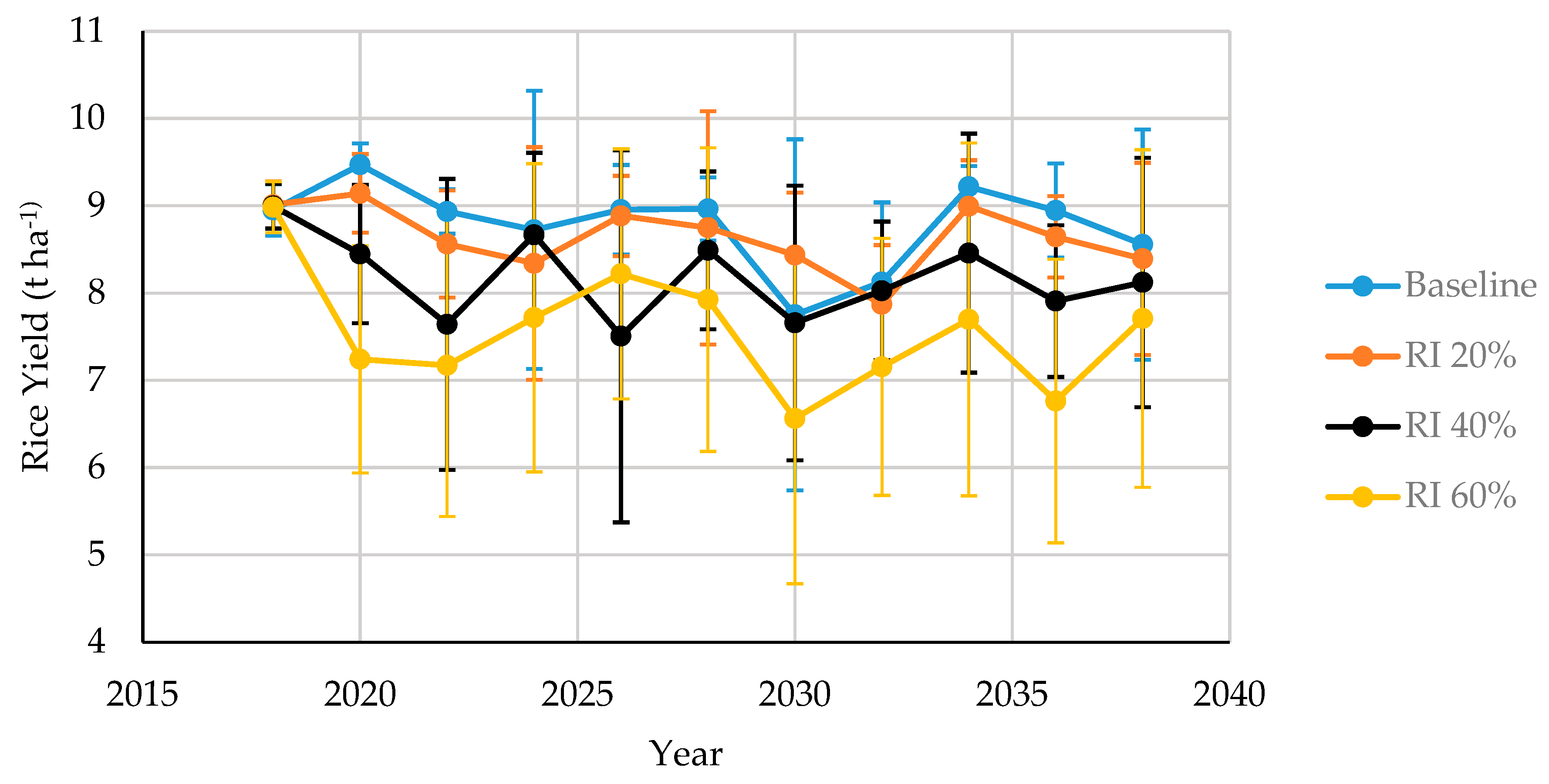
3.3. Limiting Irrigation Scenario

The goal of simulating increasingly limited irrigation scenarios was to find the threshold at which the effect of water stress on yield became significant and determine whether water was being wasted in the current management strategy. The results varied for each field (

Table 8. Average rice yields for baseline (the farmer’s input in 2018 and 2019) and reduced irrigation (RI) scenarios for 2018–2038.

Field	Baseline	RI 10%	RI 20%	RI 30%	RI 40%	RI 50%	RI 60%
R2-AWD	9.10 a	9.05 a	9.00 a	8.90 a	8.56 ab	8.78 a	8.50 b
R3-AWD	8.27 a	8.31 a	8.11 a	8.12 ab	7.79 b	7.30 c	6.73 d
R5-FIR	9.37 a	9.36 a	9.25 b	8.82 bc	8.72 c	8.61 c	8.29 d
R7-CVF	8.52 a	8.57 a	8.66 ab	8.65 ab	8.88 b	9.04 bc	8.93 c
R8-AWD	8.65 a	8.33 a	8.17 a	7.72 b	6.91 c	6.07 d	5.35 e
All	8.78 a	8.72 a	8.64 a	8.44 a	8.17 a	7.96 a	7.56 b

Note: Superscripts of different letters across the same row denote a significant difference at α = 0.05 using the paired t-test. RI—reduced irrigation, AWD—alternate wetting and drying, FIR—furrow irrigation for rice, CVF—conventional flooding. Values of 10, 20, 30, 40, 50, and 60% are the amounts by which irrigation was reduced. “All” refers to all of the fields averaged together.

). Among the three AWD fields, R2, R3, and R8 had significant yield decrease at 60, 40, and 30% reduced irrigation, respectively. The only FIR field (R5) had a significant yield decrease at 20% irrigation. The only CVF field (R7) had a significant yield increase starting at 40%. Yield decreases were generally considered significant when they reached a ~5% reduction (

Table 9. Percent average rice yield change of each reduced irrigation scenario compared to the baseline (the farmer’s input in 2018).

Field	RI 10%	RI 20%	RI 30%	RI 40%	RI 50%	RI 60%
R2-AWD	−0.55	−1.10	−2.20	−5.93	−3.52	−6.59
R3-AWD	0.48	−1.93	−1.81	−5.80	−11.73	−18.62
R5-FIR	−0.11	−1.28	−5.87	−6.94	−8.11	−11.53
R7-CF	0.59	1.64	1.53	4.23	6.10	4.81
R8-AWD	−3.70	−5.55	−10.75	−20.12	−29.83	−38.15
All	−0.66	−1.64	−3.87	−6.95	−9.36	−13.91

Note: RI—reduced irrigation, AWD—alternate wetting and drying, FIR—furrow irrigation for rice, CF—continuous flood. Values of 10, 20, 30, 40, 50, and 60% are the amounts by which irrigation was reduced. “All” refers to all of the fields averaged together. Percent change is calculated ((RI-baseline)/baseline) *100%).

). These scenarios provoked only minor changes in nitrogen stress days, with the only statistically significant difference in R7, starting at 40% reduced irrigation (

Table A1. Average nitrogen stress days on rice for baseline (i.e., using the farmer’s input in 2018) and reduced irrigation (RI) scenarios for years 2018–2038.

Field	Baseline	RI 10%	RI 20%	RI 30%	RI 40%	RI 50%	RI 60%
R2-AWD	19 a	20 a	20 a	21 a	23 a	17 a	17 a
R3-AWD	31 a	30 a	30 a	26 a	26 a	25 a	22 a
R5-FIR	3 a	2 a	2 a	6 a	4 a	2 a	2 a
R7-CF	15 a	15 a	13 a	13 ab	10 b	8 b	8 b
R8-AWD	18 a	29 a	27 a	24 a	24 a	24 a	22 a
All	17 a	19 a	18 a	18 a	17 a	15 a	14 a

Note: Superscripts of different letters across the same row denote a significant difference at α = 0.05 using the paired t-test. RI—reduced irrigation, AWD—alternate wetting and drying, FIR—furrow irrigation for rice, CF—continuous flood. Values of 10, 20, 30, 40, 50, and 60% are the amounts by which irrigation was reduced.

). The water stress in R3, R5, and R8 was significant for each reduced irrigation (

Table A2. Average water stress days on rice for baseline (i.e., using the farmer’s input in 2018) and reduced irrigation (RI) scenarios for years 2018–2038.

Field	Baseline	RI 10%	RI 20%	RI 30%	RI 40%	RI 50%	RI 60%
R2-AWD	1 a	1 a	2 a	3 b	7 c	10 d	13 e
R3-AWD	11 a	12 b	15 c	21 d	26 e	33 f	40 g
R5-FIR	4 a	6 b	8 c	11 d	14 e	18 f	22 g
R7-CF	6 a	6 a	6 a	6 a	6 a	6 a	11 b
R8-AWD	0 a	6 b	14 c	25 d	34 e	43 f	52 g
All	4 a	6 b	9 c	13 d	17 e	22 f	27 g

Note: Superscripts of different letters across the same row denote a significant difference at α = 0.05 using the paired t-test. RI—reduced irrigation, AWD—alternate wetting and drying, FIR—furrow irrigation for rice, CF—continuous flood. Values of 10, 20, 30, 40, 50, and 60% are the amounts by which irrigation was reduced.

). The water stress in R2 and R7 became significant at 30 and 60% reduced irrigation, respectively (Table A2).

The general effect of reduced irrigation was a reduction in yield (Figure 3). The opposite was true, however, in R7, which consistently had increased yield compared to the baseline. Two fields, R5 and R8, both had consistently decreasing yield with reduced irrigation. The R2 and R3 fields also had general patterns of decreasing yield, with the exception that reductions in the range of 10–30% were relatively minor (<3%). The largest overall effect was in R8, possibly because of the high plant density (Table 2), increasing competition for resources between the plants. Moreover, a significant yield drop was observed in the years 2030 and 2032, which was due to less rainfall and more nitrogen stress in those two years (Figure A1).

4. Discussion

4.1. Calibration and Validation

Upon running a t-test assuming unequal variances, observed yields of both rice and soybean were not significantly different from the simulated yields at α = 0.05. The model did not consistently over or underpredict rice or soybean yields, and the PBIAS was well within the 25% limit deemed satisfactory by Wang et al. [40] and was comparable to those obtained in other studies using APEX [59] and EPIC [56]. The overall E value was smaller in rice (−0.22) compared to soybean (0.38) and was lower than that obtained by Gilardelli et al. using the Water Accounting Rice Model (WARM) [60]. The percent difference between the mean of simulated and observed rice yields was −2.47%, and that of soybean yields was 11.87%, indicating very good calibration. For reference, the yields simulated by Williams et al. [38] using EPIC were all within 7% of observed yields. It is important to note that the calibration was based solely on two years for which data were available, one for rice and one for soybean. Including more years may have made for a more robust calibration. The agreement in the MODIS and APEX LAI was also a great achievement. Ren et al. [27] also used MODIS data to compare with the EPIC model at a global scale and concluded that it is feasible to use this method.

4.2. Crop Rotation Scenarios

Given that the rice–rice rotation yields were higher in three of the five simulated fields, the results of the simulation may suggest that a rice–rice rotation leads to higher yields compared to the soybean–rice rotation. According to the paired t-tests, however, none of the differences in yield were significant. Additionally, based on the simulation, there were large differences in nitrogen stress in three of the fields, although it was not consistent whether the rice–rice rotation increased or decreased stress. Again, none of the results on nitrogen stress were statistically significant. Although Anders et al. [61] conclude that including soybean in rotation with rice increases both rice yield and nitrogen uptake, Peoples et al. [6] report that the benefits of nitrogen fixation by soybean may be minimal because most of the absorbed nitrogen is removed at harvest. Other studies state that including soybean in the rotation does decrease the need for nitrogen fertilizer, if only marginally [62]. Another factor in the nitrogen stress analysis is that the soybean in soybean–rice rotation did not include any nitrogen application. The modeled nitrogen fixation by soybean may have been able to make up for this deficit in some fields and not in others. Weed and pest management should also be considered. Filizadeh et al. [7] and Scherner et al. [5] both attest to the benefits of the soybean–rice rotation with regard to limiting weed growth and pest development.

4.3. Limiting Irrigation Scenarios

The results showed a decrease in yield with reduced irrigation in all fields except R7, which is the only field considered to be in continuous flood rather than AWD, as can be seen in the large discrepancy in irrigation amounts applied to those fields (Table 2). One notable aspect of R7 is that the baseline irrigation amount (1649 mm) is almost twice that of the next highest field (751 mm); this field was over-irrigated. A typical irrigation amount for CVF rice is around 818 mm [10].

The three AWD fields, R2, R3, and R8, responded differently in the percent yield change (Table 9). Starting at RI 30%, the R8 field reduced its yield by 10% for every 10% reduction in irrigation. This might be due to the highest plant density in R8 compared to other fields. Ahmad et al. [63] assert that, indeed, density related competition between plants can affect yield and water use efficiency. The results in R8 seem to be close to those of Yang et al. [64], who found that severe AWD with 38 to 50% reduced irrigation caused a yield reduction of 19 to 35%. However, Yao et al. [65] and Rejesus et al. [16] found that using AWD with 38% reduced irrigation did not significantly reduce yield compared to continuous flood. In this study, reducing up to 20% water use only caused less than 2% yield change in all fields, except R8. Other studies have also been able to reduce irrigation by 15% [66] and 28% [67] without affecting yield. Tabbal et al. [68] even assert that, if soil saturation is maintained and weed control is adequate, irrigation could be reduced by 40% or more, compared to traditional shallow flooding, without affecting yield.

Reducing irrigation seemed to affect nitrogen stress as well, although the pattern was not consistent in each field. In some fields (R3 and R7), nitrogen stress consistently decreased with reduced irrigation, and R7 had the most nitrogen lost to denitrification as simulated by APEX compared to the other fields of the baseline irrigation. Indeed, Yang et al. [69] conclude that controlling irrigation is an effective method of reducing nitrogen loss to the environment. These effects on nitrogen stress could partly explain why the pattern of yield decrease was less clear in R3 and why the yield tended to increase with reduced irrigation in R7. The results in R3 and R7 could indicate that, in some cases, reducing irrigation not only saves water but may also increase yield. The response of rice yield to reduced irrigation is also dependent on environmental factors, such as precipitation, temperature, and soil, so results vary and direct comparisons may be misleading.

The results of R5, the only FIR field, seemed to be affected most by smaller reductions in irrigation. The R5 results could indicate that FIR is more sensitive to irrigation reduction compared to flooded rice. FIR also had lower yields compared to flooded rice in studies from Arkansas [70] and Australia [71]. Henry et al. [9] also stated that maintaining yield can be difficult with furrow irrigated rice. It is also interesting that the FIR field had so much less nitrogen stress than the other fields, probably because it had the highest amount of nitrogen input compared to other fields and less runoff.

5. Conclusions and Future Studies

Although an independent validation test was not performed for the rice model due to limitations in the observed data, APEX was able to model rice yields based on the calibration results of the yield and LAI. The scenarios in crop rotation showed that there was no statistically significant difference between the soybean–rice and rice–rice systems. Although the results were not significant, they could still have long-term implications concerning profits to the farmers, especially over a longer period, but a detailed economic analysis would be needed to determine whether a long-term rice–rice rotation poses any economic benefits.

The reduced irrigation scenario showed a decrease in yield with decreased irrigation, except for the R7 field, which was over-irrigated. These results raise questions about the detriments of over-irrigation, such as increased nitrogen loss, which could be examined more closely in future studies. The results in R8 also raise questions about whether high plant density can cause a negative effect on yield, which could also be examined more closely in future studies. Furthermore, more detailed future studies could test the effects of different irrigation methods on crop nitrogen stress and consider how these differences can be represented in models.

References

1. Hardke, J.T. Trends in Arkansas Rice Production, 2018; Arkansas Agricultural Experiment Station, University of Arkansas System: Fayetteville, AR, USA, 2019; pp. 15–24. [Google Scholar]
2. Arkansas Farm Bureau. Ag Facts. Available online: https://www.arfb.com/pages/education/ag-facts/ (accessed on 30 May 2020).
3. USDA-NASS. Arkansas Acreage; Delta Region—Arkansas Field Office: Little Rock, AR, USA, 28 June 2019; p. 2.
4. Watkins, K.B.; Anders, M.M.; Windham, T.E. An economic comparison of alternative rice production systems in Arkansas. J. Sustain. Agric. 2004, 24, 57–78. [Google Scholar] [CrossRef]
5. Scherner, A.; Schreiber, F.; Andres, A.; Concenço, G.; Martins, M.B.; Pitol, A. Rice Crop Rotation: A Solution for Weed Management. Developments 2018, 83. [Google Scholar] [CrossRef]
6. Peoples, M.; Brockwell, J.; Herridge, D.; Rochester, I.; Alves, B.; Urquiaga, S.; Boddey, R.; Dakora, F.; Bhattarai, S.; Maskey, S. The contributions of nitrogen-fixing crop legumes to the productivity of agricultural systems. Symbiosis 2009, 48, 1–17. [Google Scholar] [CrossRef]
7. Filizadeh, Y.; Rezazadeh, A.; Younesi, Z. Effects of crop rotation and tillage depth on weed competition and yield of rice in the paddy fields of Northern Iran. J. Agric. Sci. Technol. 2007, 9, 99–105. [Google Scholar]
8. Smith, M.; Massey, J.; Branson, J.; Epting, J.; Pennington, D.; Tacker, P.; Thomas, J.; Vories, E.; Wilson, C. Water use estimates for various rice production systems in Mississippi and Arkansas. Irrig. Sci. 2007, 25, 141–147. [Google Scholar] [CrossRef]
9. Henry, C.; Daniels, M.; Hamilton, M.; Hardke, J. Water Management. In Arkansas Rice Production Handbook; University of Arkansas Division of Agriculture: Little Rock, AR, USA, 2018; pp. 103–128. [Google Scholar]
10. Henry, C.; Hirsh, S.L.; Anders, M.M.; Vories, E.D.; Reba, M.L.; Watkins, K.B.; Hardke, J.T. Annual Irrigation Water Use for Arkansas Rice Production. J. Irrig. Drain. Eng. 2016, 142, 05016006. [Google Scholar] [CrossRef]
11. Massey, J.H.; Smith, M.C.; Vieira, D.A.N.; Adviento-Borbe, M.A.; Reba, M.L.; Vories, E.D. Expected Irrigation Reductions Using Multiple-Inlet Rice Irrigation under Rainfall Conditions of the Lower Mississippi River Valley. J. Irrig. Drain. Eng. 2018, 144, 04018016. [Google Scholar] [CrossRef]
12. USGS. Irrigation Methods: Furrow or Flood Irrigation. Available online: https://www.usgs.gov/special-topic/water-science-school/science/irrigation-methods-furrow-or-flood-irrigation?qt-science_center_objects=0#qt-science_center_objects (accessed on 10 January 2019).
13. Barber, T.; Bateman, N.; Butts, T.; Hamilton, M.; Henry, C.; Lorenz, G.; Mazzanti, R.; Norsworthy, J.; Roberts, T.; Wamishe, Y.; et al. Arkansas Furrow-Irrigated Rice Handbook. Available online: https://www.uaex.edu/farm-ranch/crops-commercial-horticulture/rice/ArkansasFurrowIrrigatedRiceHandbook.pdf (accessed on 22 May 2020).
14. Rai, R.K.; Singh, V.P.; Upadhyay, A. Irrigation Methods. In Planning and Evaluation of Irrigation Projects; Academic Press: New York, NY, USA, 2017; pp. 353–363. [Google Scholar]
15. Nelson, A.; Wassmann, R.; Sander, B.O.; Palao, L.K. Climate-Determined Suitability of the Water Saving Technology “Alternate Wetting and Drying” in Rice Systems: A Scalable Methodology demonstrated for a Province in the Philippines. PLoS ONE 2015, 10, e0145268. [Google Scholar] [CrossRef]
16. Rejesus, R.M.; Palis, F.G.; Rodriguez, D.G.P.; Lampayan, R.M.; Bouman, B.A.M. Impact of the alternate wetting and drying (AWD) water-saving irrigation technique: Evidence from rice producers in the Philippines. Food Policy 2011, 36, 280–288. [Google Scholar] [CrossRef]
17. Pandey, S.; Byerlee, D.; Dawe, D.; Dobermann, A.; Mohanty, S.; Rozelle, S.; Hardy, B. Rice in the Global Economy: Strategic Research and Policy Issues for Food Security; International Rice Research Institute: Los Banos, Phillipines, 2010. [Google Scholar]
18. Nalley, L.; Linquist, B.; Kovacs, K.; Anders, M. The Economic Viability of Alternative Wetting and Drying Irrigation in Arkansas Rice Production. Agron. J. 2015, 107, 579–587. [Google Scholar] [CrossRef] [Green Version]
19. Runkle, B.R.; Suvočarev, K.; Reba, M.L.; Reavis, C.W.; Smith, S.F.; Chiu, Y.-L.; Fong, B. Methane emission reductions from the alternate wetting and drying of rice fields detected using the eddy covariance method. Environ. Sci. Technol. 2018, 53, 671–681. [Google Scholar] [CrossRef] [PubMed]
20. Carrijo, D.R.; Lundy, M.E.; Linquist, B.A. Rice yields and water use under alternate wetting and drying irrigation: A meta-analysis. Field Crop. Res. 2017, 203, 173–180. [Google Scholar] [CrossRef]
21. Lampayan, R.M.; Bouman, B.A.M.; Palis, F.G.; Flor, R.J. Paper 14 Developing and Disseminating Alternate Wetting and Drying Water-Saving Technology in the Philippines; Technical Report; Asian Development Bank: Mandaluyong, Philippines, 2016; pp. 337–360. [Google Scholar]
22. Gassman, P.W.; Williams, J.R.; Wang, X.; Saleh, A.; Osei, E.; Hauck, L.M.; Izaurralde, R.C.; Flowers, J.D. The Agricultural Policy/Environmental eXtender (APEX) Model: An Emerging Tool for Landscape and Watershed Environmental Analysis. Trans. ASABE 2010, 53, 711–740. [Google Scholar] [CrossRef] [Green Version]
23. Zhao, J.; Chu, Q.; Shang, M.; Meki, M.N.; Norelli, N.; Jiang, Y.; Yang, Y.; Zang, H.; Zeng, Z.; Jeong, J. Agricultural Policy Environmental eXtender (APEX) Simulation of Spring Peanut Management in the North China Plain. Agronomy 2019, 9, 443. [Google Scholar] [CrossRef] [Green Version]
24. Bosch, D.D.; Doro, L.; Jeong, J.; Wang, X.; Williams, J.R.; Pisani, O.; Endale, D.M.; Strickland, T.C. Conservation tillage effects in the Atlantic Coastal Plain: An APEX examination. J. Soil Water Conserv. 2020, 75, 400–415. [Google Scholar] [CrossRef]
25. Williams, J.R.; Arnold, J.G.; Srinivasan, R.; Ramanarayanan, T.S. APEX: A New Tool for Predicting the Effects of Climate and CO2 Changes on Erosion and Water Quality. Springer-Verl. Nato-Asi Glob. Chang. Ser. Heidelb. Ger. 1998, 1, 441–449. [Google Scholar]
26. ORNL-DAAC. MODIS and VIIRS Land Products Global Subsetting and Visualization Tool; ORNL DAAC: Oak Ridge, TN, USA, 2018. [Google Scholar]
27. Ren, J.; Yu, F.; Qin, J.; Chen, Z.; Tang, H. Integrating remotely sensed lai with epic model based on global optimization algorithm for regional crop yield assessment. In Proceedings of the 2010 IEEE International Geoscience and Remote Sensing Symposium, Honolulu, HI, USA, 25–30 July 2010; pp. 2147–2150. [Google Scholar]
28. Trombetta, A.; Iacobellis, V.; Tarantino, E.; Gentile, F. Calibration of the AquaCrop model for winter wheat using MODIS LAI images. Agric. Water Manag. 2016, 164, 304–316. [Google Scholar] [CrossRef]
29. USDA-NRCS. Web Soil Survey. Available online: https://websoilsurvey.sc.egov.usda.gov/App/WebSoilSurvey.aspx (accessed on 30 September 2019).
30. Google Earth. Google Earth. Available online: https://www.google.com/earth/ (accessed on 15 January 2020).
31. Hardke, J.; Baker, R.; Barber, T.; Henry, C.; Lorenz, G.; Mazzanti, R.; Norman, R.; Norsworthy, J.; Roberts, T.; Scott, B.; et al. Rice Farming for Profit; University of Arkansas Division of Agriculture: Little Rock, AR, USA, 2017. [Google Scholar]
32. Hardke, J.; Moldenhauer, K.; Sha, X. Rice Cultivars and Seed Production; University of Arkansas, Division of Agriculture Research & Extension, University of Arkansas Division of Agriculture Cooperative Extension Service: Little Rock, AR, USA, 2013; pp. 21–28. [Google Scholar]
33. Ashlock, L.; Klerk, R.; Huitink, G.; Keisling, T.; Vories, E. Planting Practices. In Arkansas Soybean Handbook; University of Arkansas Division of Agriculture: Little Rock, AR, USA, 2014. [Google Scholar]
34. USDA-NRCS. Residue and Tillage Management, Reduced Till. Available online: https://www.nrcs.usda.gov/wps/portal/nrcs/detail/?cid=nrcs144p2_027126 (accessed on 10 October 2019).
35. USDA-NRCS. Residue and Tillage Management, No Till. Available online: https://www.nrcs.usda.gov/wps/portal/nrcs/detail/?cid=nrcs144p2_027119 (accessed on 10 October 2019).
36. Tacker, P.; Vories, E. Irrigation. In Arkansas Soybean Handbook; University of Arkansas Division of Agriculture: Little Rock, AR, USA, 2014. [Google Scholar]
37. Flowers, J.D.; Williams, J.R.; Hauck, L.M. NPP Integrated Modeling System: Calibration of the APEX Model for Dairy Waste Application Fields in Erath County, Texas; Texas Institute for Applied Environmental Research, Tarleton State University: Tarleton, TX, USA, 1996. [Google Scholar]
38. Williams, J.R.; Jones, C.A.; Kiniry, J.R.; Spanel, D.A. The EPIC crop growth model. Trans. ASAE 1989, 32, 497–511. [Google Scholar] [CrossRef]
39. Williams, J.R.; Izaurralde, R.C.; Steglich, E.M. Agricultural policy/environmental extender model. Theor. Doc. Version 2008, 604, 2008–2017. [Google Scholar]
40. Wang, X.; Williams, J.R.; Gassman, P.W.; Baffaut, C.; Izaurralde, R.C.; Jeong, J.; Kiniry, J.R. EPIC and APEX: Model Use, Calibration, and Validation. Trans. ASABE 2012, 55, 1447–1462. [Google Scholar] [CrossRef]
41. Cavero, J.; Barros, R.; Sellam, F.; Topcu, S.; Isidoro, D.; Hartani, T.; Lounis, A.; Ibrikci, H.; Cetin, M.; Williams, J. APEX simulation of best irrigation and N management strategies for off-site N pollution control in three Mediterranean irrigated watersheds. Agric. Water Manag. 2012, 103, 88–99. [Google Scholar] [CrossRef] [Green Version]
42. Prada, A.F.; Chu, M.L.; Guzman, J.A.; Moriasi, D.N. Evaluating the impacts of agricultural land management practices on water resources: A probabilistic hydrologic modeling approach. J. Environ. Manag. 2017, 193, 512–523. [Google Scholar] [CrossRef] [PubMed] [Green Version]
43. Zhang, B.; Feng, G.; Read, J.J.; Kong, X.; Ouyang, Y.; Adeli, A.; Jenkins, J.N. Simulating soybean productivity under rainfed conditions for major soil types using APEX model in East Central Mississippi. Agric. Water Manag. 2016, 177, 379–391. [Google Scholar] [CrossRef] [Green Version]
44. David, L.B.; Theodor, S.S.; Albert, J.C.; Joon Hee, L. The Current State of Predicting Furrow Irrigation Erosion. In Proceedings of the 5th National Decennial Irrigation Conference Proceedings, Phoenix Convention Center, Phoenix, AZ, USA, 5–8 December 2010. [Google Scholar]
45. Francesconi, W.; Smith, D.D.; Heathman, G.; Williams, C.; Wang, X. Monitoring and APEX modeling of no-till and reduced-till in tile drained agricultural landscapes for water quality. Trans. ASABE 2014, 57, 777–789. [Google Scholar] [CrossRef]
46. Saleh, A.; Niraula, R.; Marek, G.W.; Gowda, P.H.; Brauer, D.K.; Howell, T.A. Lysimetric Evaluation of the APEX Model to Simulate Daily ET for Irrigated Crops in the Texas High Plains. Trans. ASABE 2018, 61, 65–74. [Google Scholar] [CrossRef]
47. Assefa, T.; Jha, M.; Reyes, M.; Worqlul, A.W.; Doro, L.; Tilahun, S. Conservation agriculture with drip irrigation: Effects on soil quality and crop yield in sub-Saharan Africa. J. Soil Water Conserv. 2020, 75, 209–217. [Google Scholar] [CrossRef]
48. Worou, O.N.; Gaiser, T.; Saito, K.; Goldbach, H.; Ewert, F. Simulation of soil water dynamics and rice crop growth as affected by bunding and fertilizer application in inland valley systems of West Africa. Agric. Ecosyst. Environ. 2012, 162, 24–35. [Google Scholar] [CrossRef]
49. Le, K.N. Evaluation of the APEX Model for Organic and Conventional Management under Conservation and Conventional Tillage Systems; North Carolina Agricultural and Technical State University: Greensboro, NC, USA, 2011. [Google Scholar]
50. BREC. WinAPEX. Available online: https://epicapex.tamu.edu/apex/winapex/ (accessed on 9 September 2019).
51. Daly, C.; Bryant, K. PRISM Climate Group. Available online: http://www.prism.oregonstate.edu/documents/PRISM_datasets.pdf (accessed on 17 April 2020).
52. Hargreaves, G.H.; Allen, R.G. History and Evaluation of Hargreaves Evapotranspiration Equation. J. Irrig. Drain. Eng. 2003, 129, 53–63. [Google Scholar] [CrossRef]
53. Steglich, E.M.; Williams, J.R. Agricultural Policy/Environmental eXtender Model: User’s Manual Version 0604; Texas AgriLIFE Research, Texas A&M University, Blackland Research and Extension Center: Temple, TX, USA, 2008; p. 222. [Google Scholar]
54. Moriasi, D.N.; Gitau, M.W.; Pai, N.; Daggupati, P. Hydrologic and water quality models: Performance measures and evaluation criteria. Trans. ASABE 2015, 58, 1763–1785. [Google Scholar] [CrossRef] [Green Version]
55. Yang, J.; Yang, J.; Liu, S.; Hoogenboom, G. An evaluation of the statistical methods for testing the performance of crop models with observed data. Agric. Syst. 2014, 127, 81–89. [Google Scholar] [CrossRef]
56. Le, K.N.; Jeong, J.; Reyes, M.R.; Jha, M.K.; Gassman, P.W.; Doro, L.; Hok, L.; Boulakia, S. Evaluation of the performance of the EPIC model for yield and biomass simulation under conservation systems in Cambodia. Agric. Syst. 2018, 166, 90–100. [Google Scholar] [CrossRef]
57. Setiyono, T.D.; Weiss, A.; Specht, J.E.; Cassman, K.G.; Dobermann, A. Leaf area index simulation in soybean grown under near-optimal conditions. Field Crop. Res. 2008, 108, 82–92. [Google Scholar] [CrossRef] [Green Version]
58. Tagliapietra, E.L.; Streck, N.A.; da Rocha, T.S.M.; Richter, G.L.; da Silva, M.R.; Cera, J.C.; Guedes, J.V.C.; Zanon, A.J. Optimum Leaf Area Index to Reach Soybean Yield Potential in Subtropical Environment. Agron. J. 2018, 110, 932–938. [Google Scholar] [CrossRef] [Green Version]
59. Choi, S.-K.; Jeong, J.; Kim, M.-K. Simulating the effects of agricultural management on water quality dynamics in rice paddies for sustainable rice production—Model development and validation. Water 2017, 9, 869. [Google Scholar] [CrossRef] [Green Version]
60. Gilardelli, C.; Stella, T.; Confalonieri, R.; Ranghetti, L.; Campos-Taberner, M.; García-Haro, F.J.; Boschetti, M. Downscaling rice yield simulation at sub-field scale using remotely sensed LAI data. Eur. J. Agron. 2019, 103, 108–116. [Google Scholar] [CrossRef]
61. Anders, M.M.; Olk, D.; Harper, T.; Daniel, T.; Holzhauer, J. The effect of rotation, tillage and fertility on rice grain yields and nutrient flows. In Proceedings of the 26th Southern Conservation Tillage Conference, Raleigh, NC, USA, 8–9 June 2004; pp. 26–29. [Google Scholar]
62. Chapman, A.; Myers, R. Nitrogen contributed by grain legumes to rice grown in rotation on the Cununurra soils of the Ord Irrigation Area, Western Australia. Aust. J. Exp. Agric. 1987, 27, 155–163. [Google Scholar] [CrossRef]
63. Ahmad, S.; Ali, H.; Shad, S.A.; Zia-ul-Haq, M.; Ahmad, A.; Maqsood, M.; Khan, M.B.; Mehmood, S.; Hussain, A. Water and radiation use efficiencies of transplanted rice (Oryza sativa L.) at different plant densities and irrigation regimes under semi-arid environment. Pak. J. Bot. 2008, 40, 199–209. [Google Scholar]
64. Yang, J.; Zhou, Q.; Zhang, J. Moderate wetting and drying increases rice yield and reduces water use, grain arsenic level, and methane emission. Crop J. 2017, 5, 151–158. [Google Scholar] [CrossRef] [Green Version]
65. Yao, F.; Huang, J.; Cui, K.; Nie, L.; Xiang, J.; Liu, X.; Wu, W.; Chen, M.; Peng, S. Agronomic performance of high-yielding rice variety grown under alternate wetting and drying irrigation. Field Crop. Res. 2012, 126, 16–22. [Google Scholar] [CrossRef]
66. Belder, P.; Bouman, B.A.M.; Cabangon, R.; Guoan, L.; Quilang, E.J.P.; Yuanhua, L.; Spiertz, J.H.J.; Tuong, T.P. Effect of water-saving irrigation on rice yield and water use in typical lowland conditions in Asia. Agric. Water Manag. 2004, 65, 193–210. [Google Scholar] [CrossRef]
67. Chapagain, T.; Yamaji, E. The effects of irrigation method, age of seedling and spacing on crop performance, productivity and water-wise rice production in Japan. Paddy Water Environ. 2010, 8, 81–90. [Google Scholar] [CrossRef]
68. Tabbal, D.; Lampayan, R.; Bhuiyan, S. Water-efficient irrigation technique for rice. In Proceedings of the Soil and Water Engineering for Paddy Field Management, AIT, Bangkok, Thailand, 28–30 January 1992; pp. 146–159. [Google Scholar]
69. Yang, S.; Peng, S.; Xu, J.; He, Y.; Wang, Y. Effects of water saving irrigation and controlled release nitrogen fertilizer managements on nitrogen losses from paddy fields. Paddy Water Environ. 2015, 13, 71–80. [Google Scholar] [CrossRef]
70. Vories, E.; Counce, P.; Keisling, T. Comparison of flooded and furrow-irrigated rice on clay. Irrig. Sci. 2002, 21, 139–144. [Google Scholar]
71. Beecher, H.; Dunn, B.; Thompson, J.; Humphreys, E.; Mathews, S.; Timsina, J. Effect of raised beds, irrigation and nitrogen management on growth, water use and yield of rice in south-eastern Australia. Aust. J. Exp. Agric. 2006, 46, 1363–1372. [Google Scholar] [CrossRef]
Figure 1. The five experimental, production-scale fields labeled with dots in Faulkner, Lonoke, and Prairie counties in Arkansas, United States.
Sustainability 12 06822 g001
Figure 2. An example of leaf area index (LAI) calibration results from 2017 to 2019 for soybean–rice–soybean at field R2. Note that the APEX model did not simulate the period between the two crops, but the MODIS image provided some values greater than zero that was likely due to grass, weed, or root biomass.
Sustainability 12 06822 g002
Figure 3. Average simulated rice yield of all fields from 2018 to 2038 under baseline irrigation and reduced irrigation (RI) percentages of 20, 40, and 60%. The error bar is the standard deviation.
Sustainability 12 06822 g003