Dynamic Pricing on Round-Trip Carsharing Services: Travel Behavior and Equity Impact Analysis through an Agent-Based Simulation


Abstract
1. Introduction
1.1. Literature Review
1.2. Research Gap
2. Materials and Methods
2.1. Scenario Setup
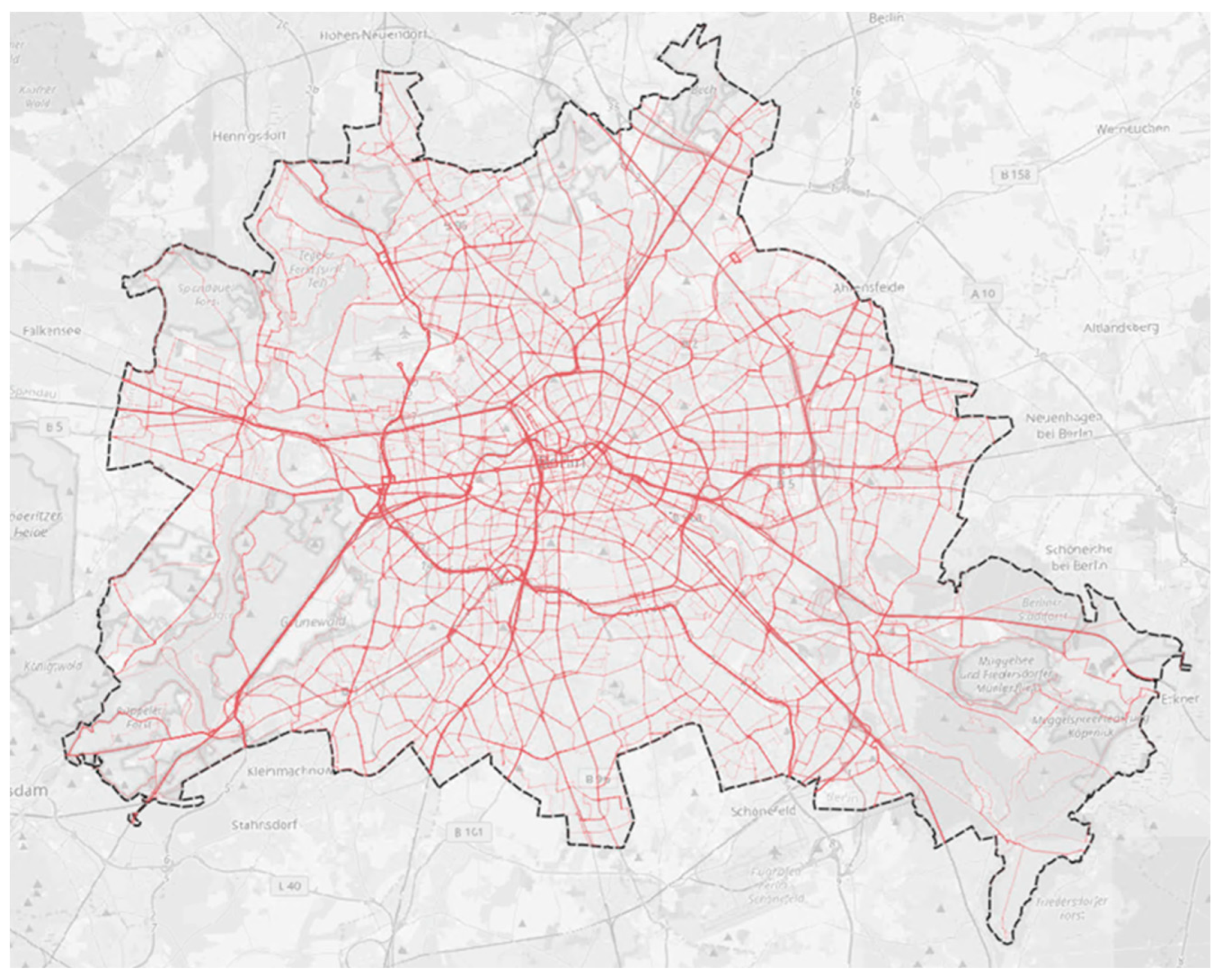
2.1.1. Network
2.1.2. Carsharing Membership
2.1.3. Configuration
2.1.4. Plans
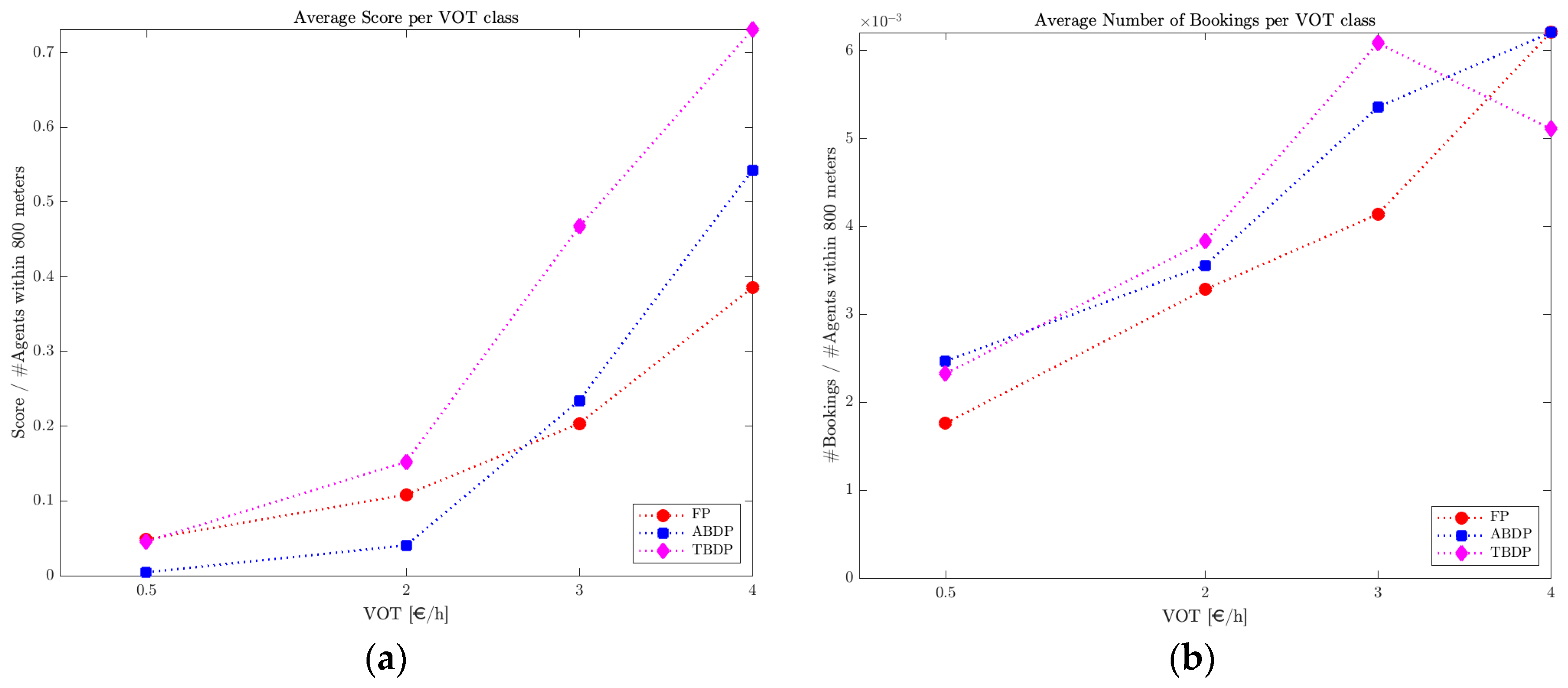
2.2. Scoring and Value of Time
2.3. Dynamic Pricing
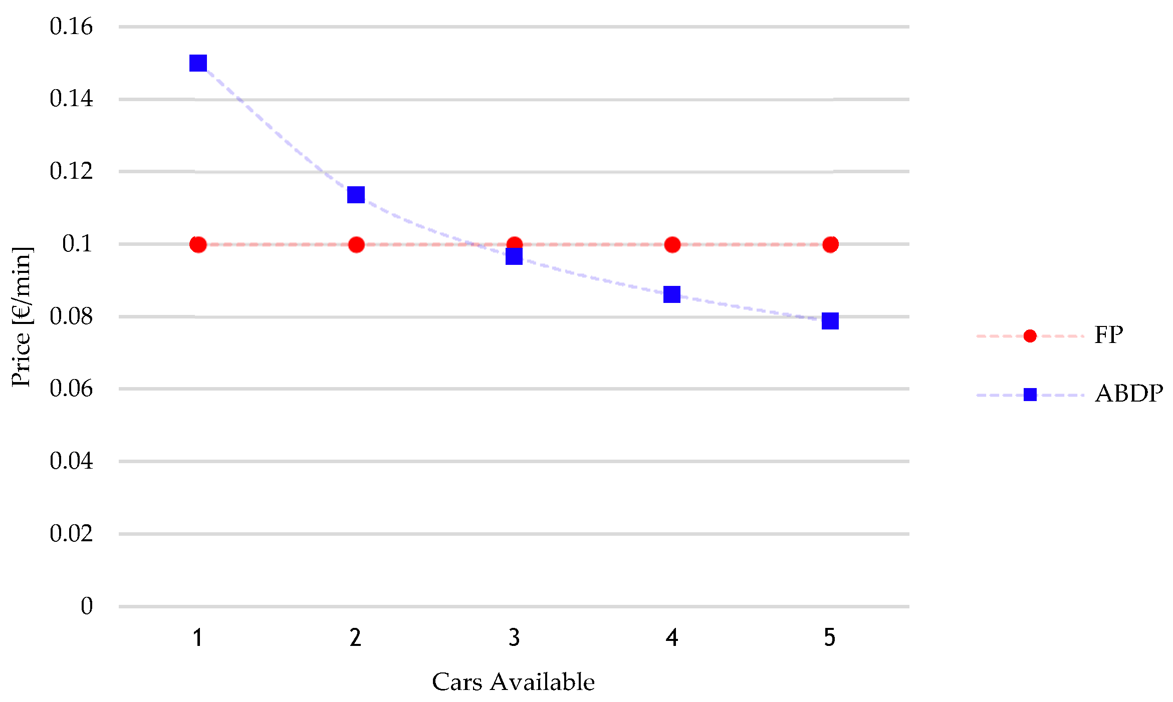
2.3.1. Availability-Based Dynamic Pricing (ABDP)
- ABDP: 0.15 . price of the last vehicle available at the station
- Fixed pricing = 0.1
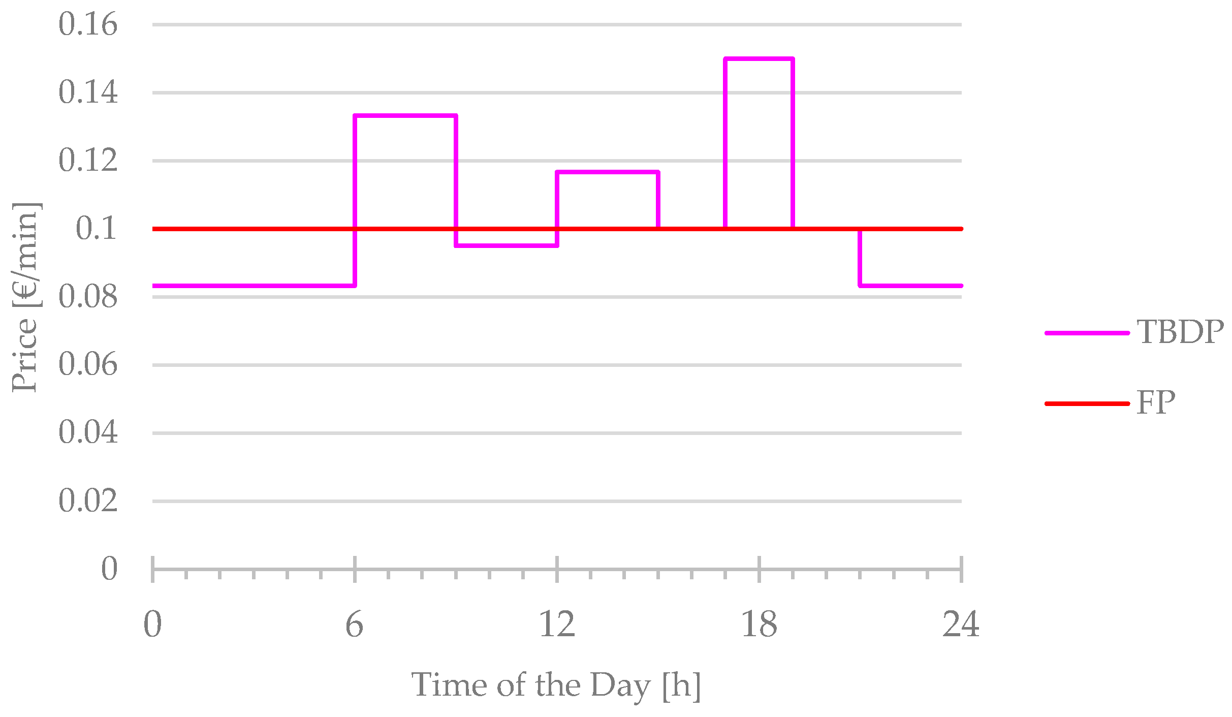
2.3.2. Time-Based Dynamic Pricing (TBDP)
3. Results
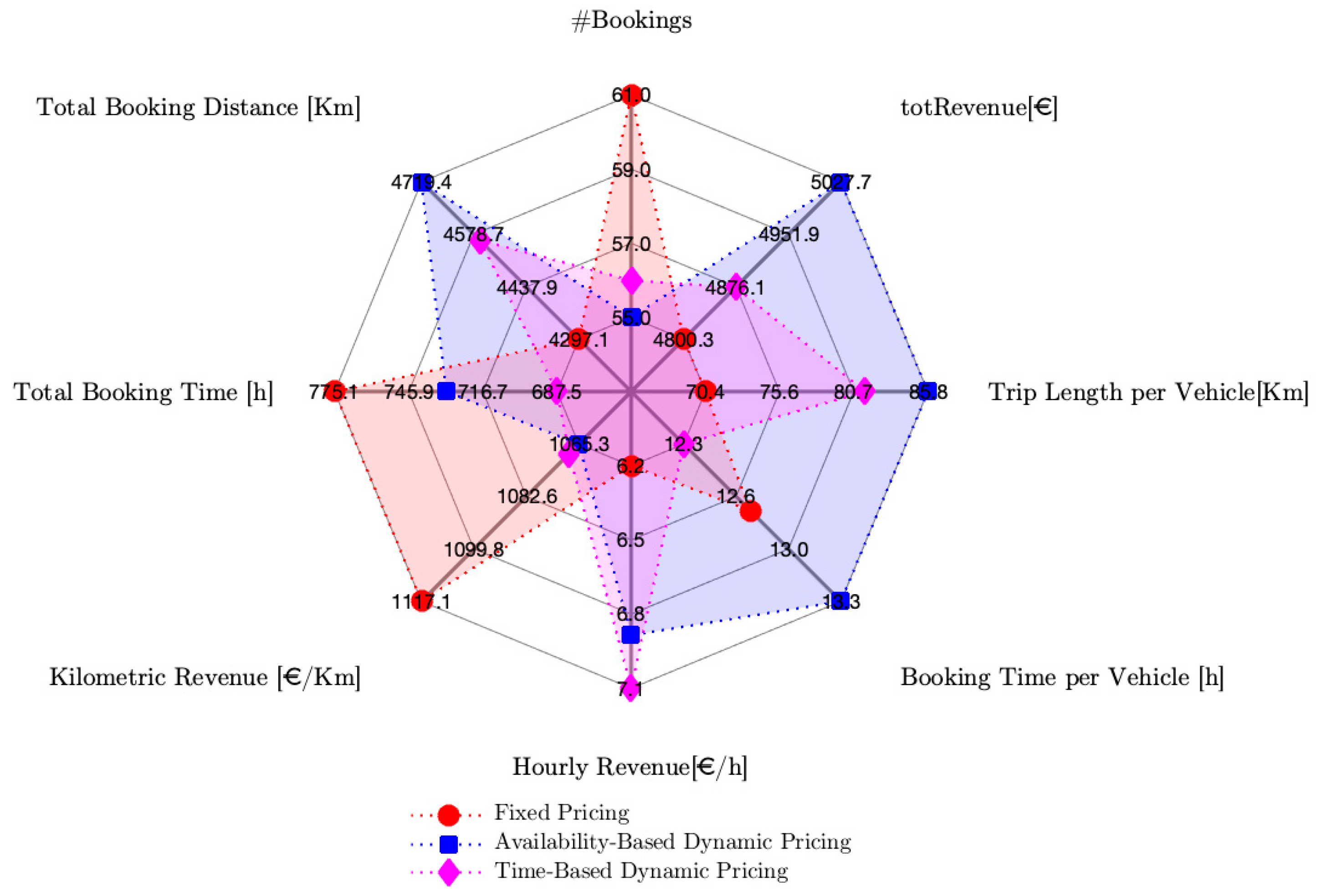
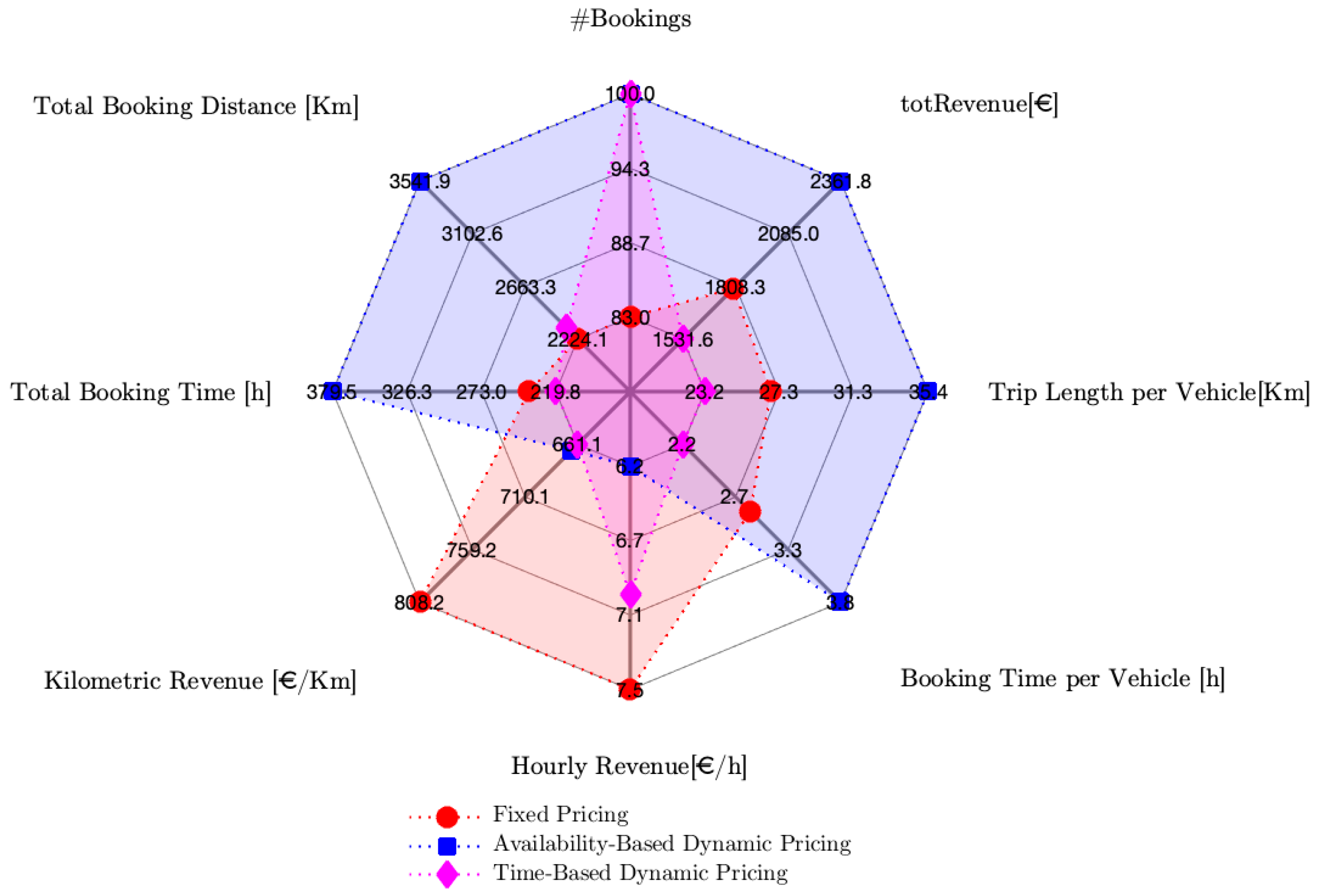
3.1. Effects on Carsharing Operations for Radial Configuration (Scenario 1)
- #Bookings: total amount of bookings for the whole day
- Tot revenue: sum of all the revenue generated during the single rents
- Trip length per vehicle: average distance traveled
- Booking time per vehicle: average booking time
- Hourly revenue: average revenue generated in one hour of booking
- Kilometric revenue: average revenue generated for every kilometer traveled
- Total booking time: sum of all the booking times
- Total booking distance: sum of all the distance traveled
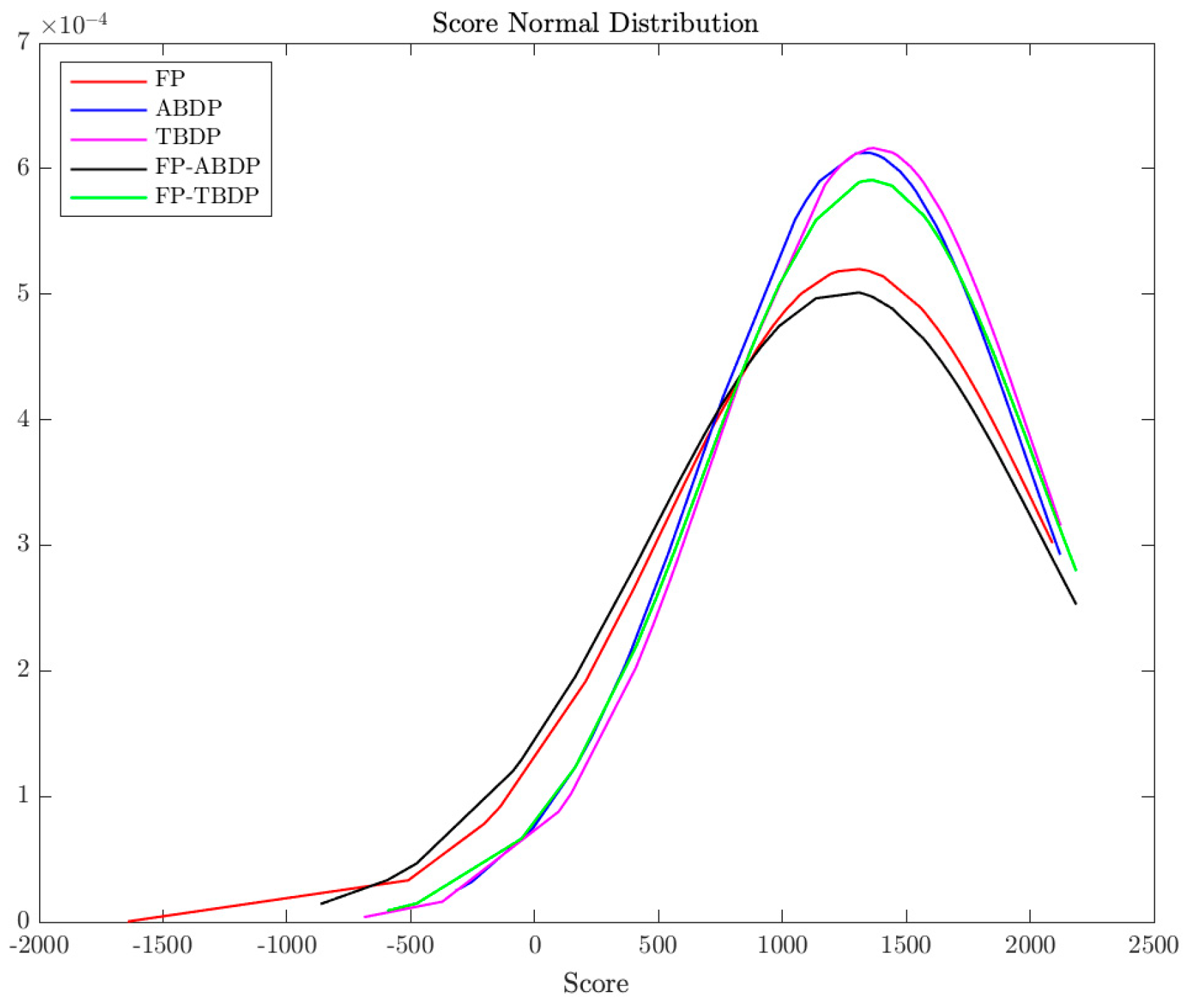
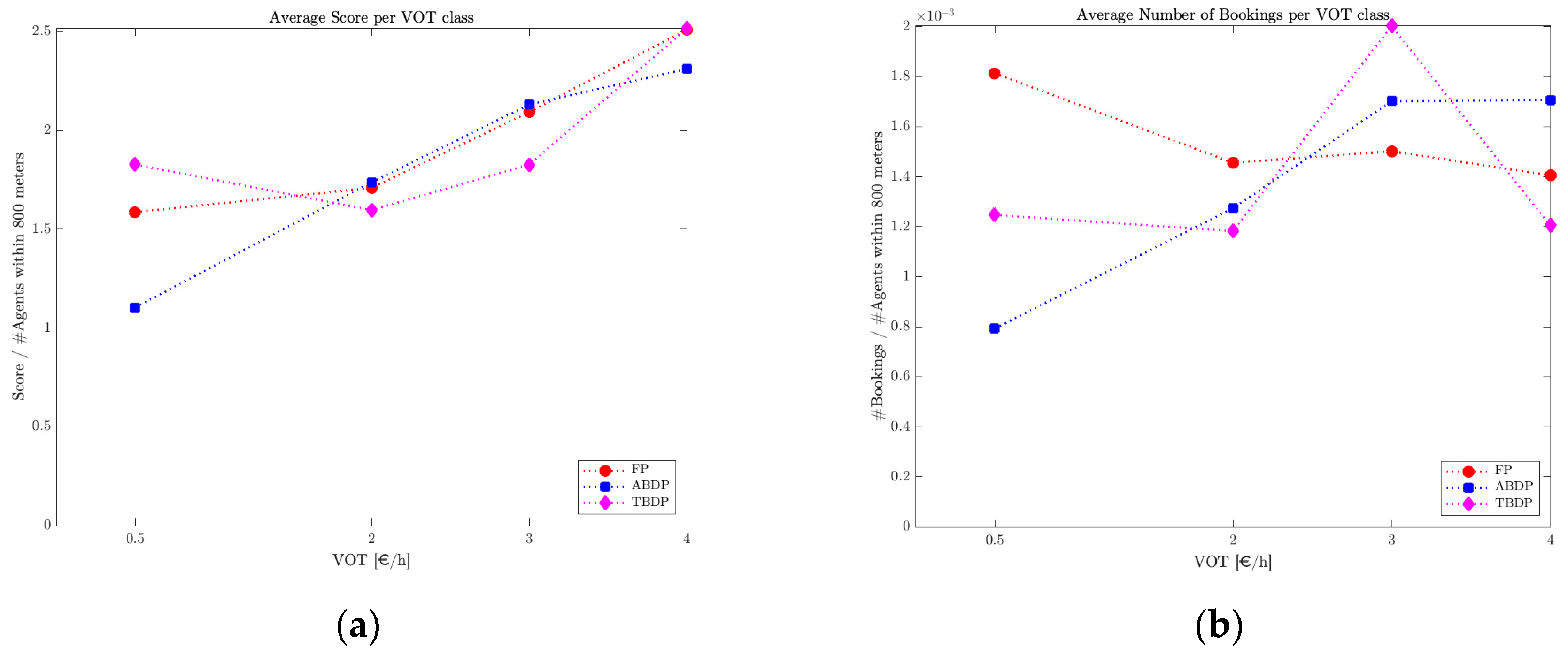
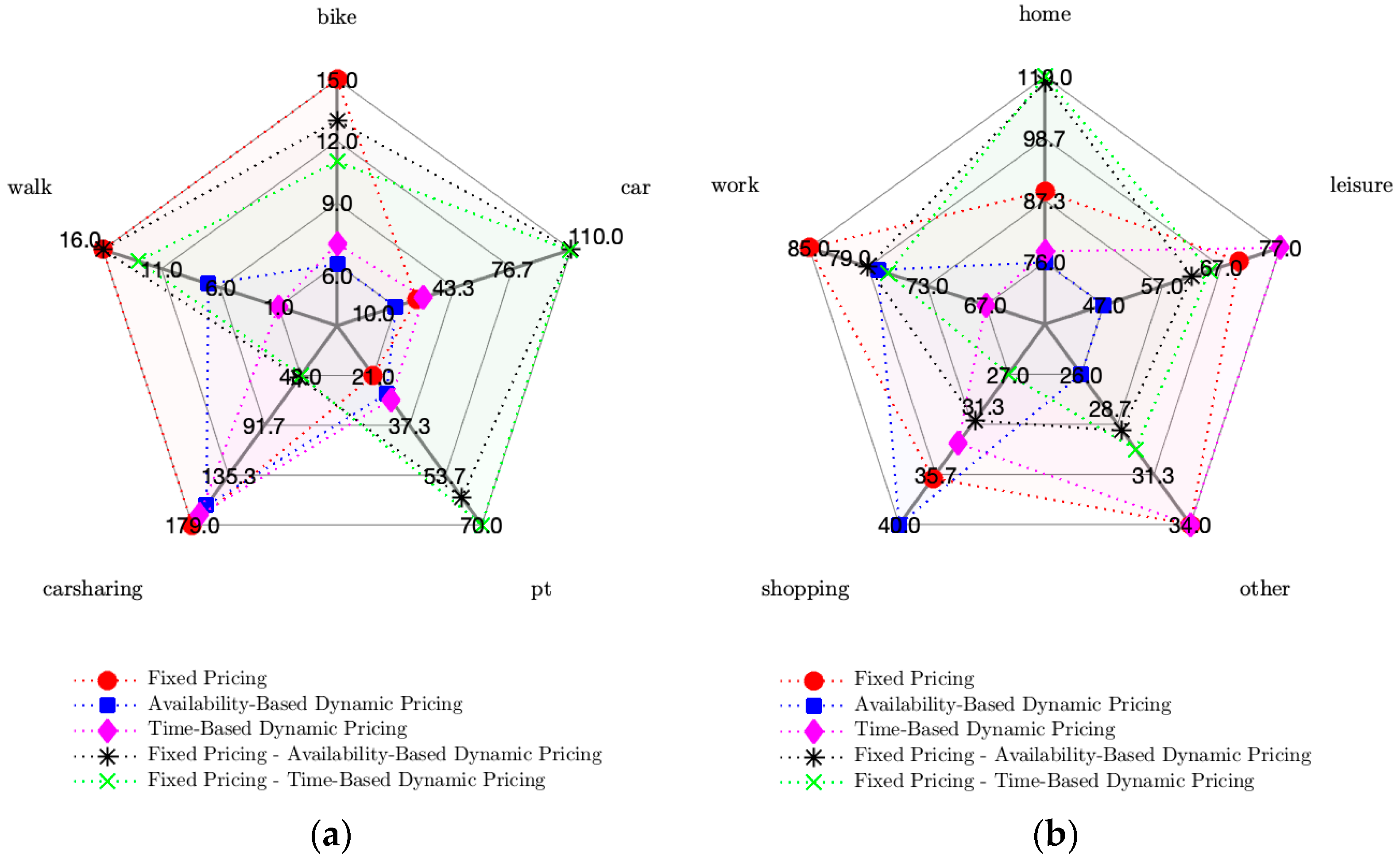
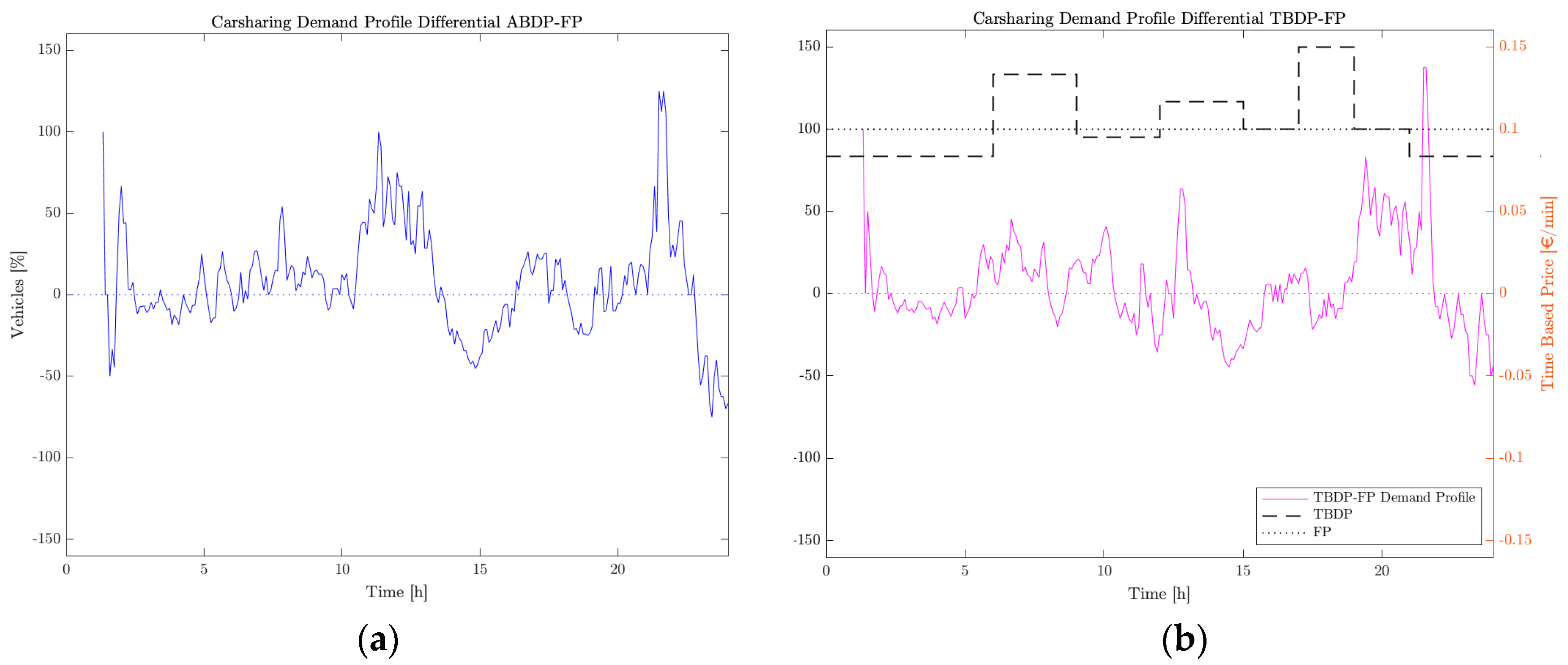
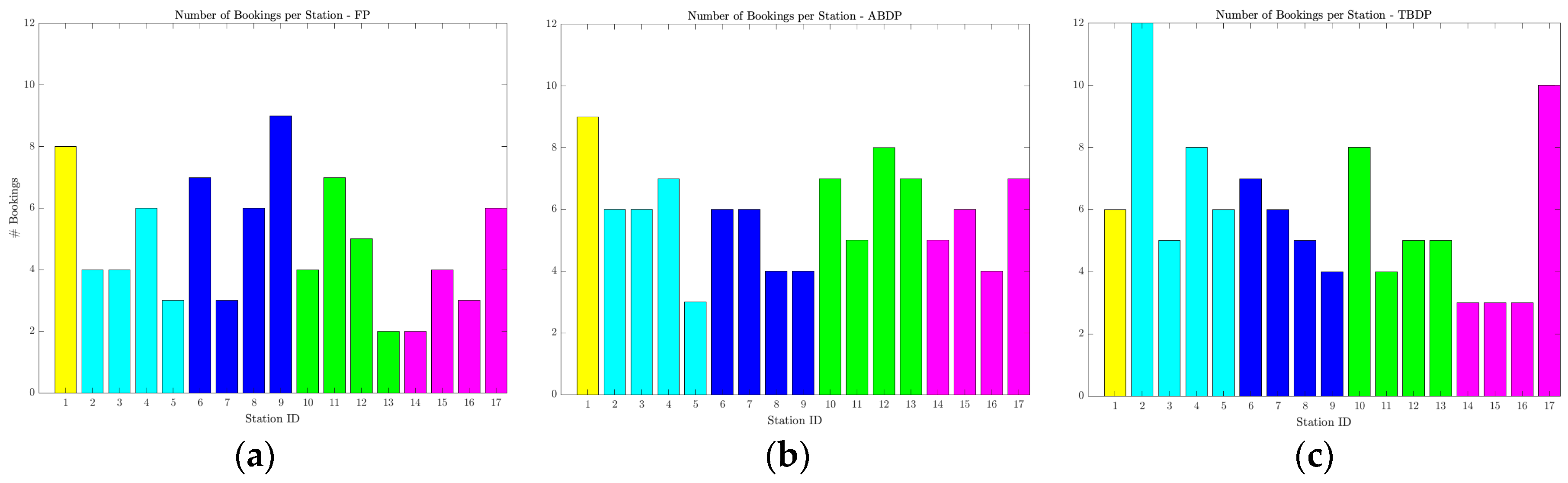
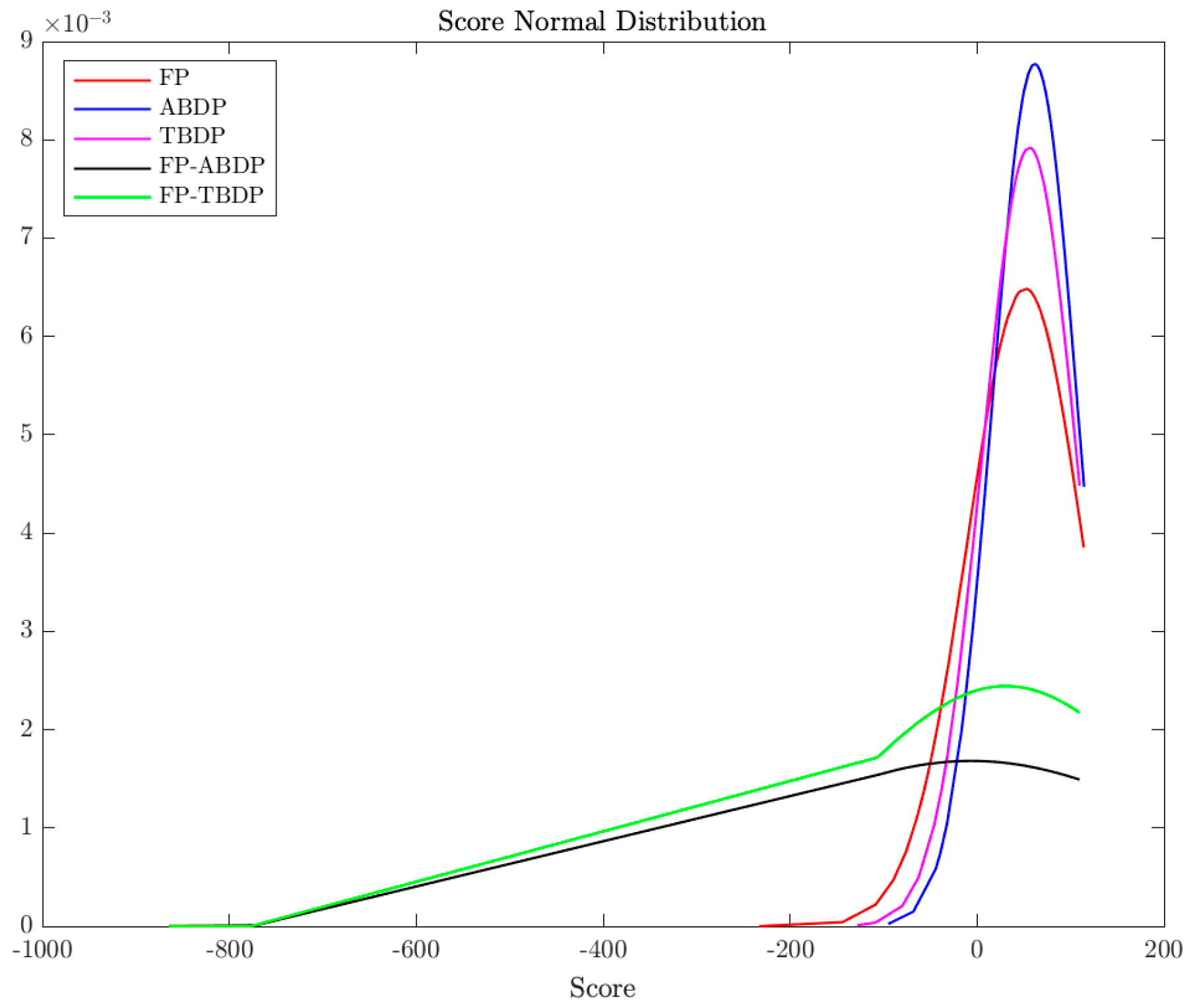
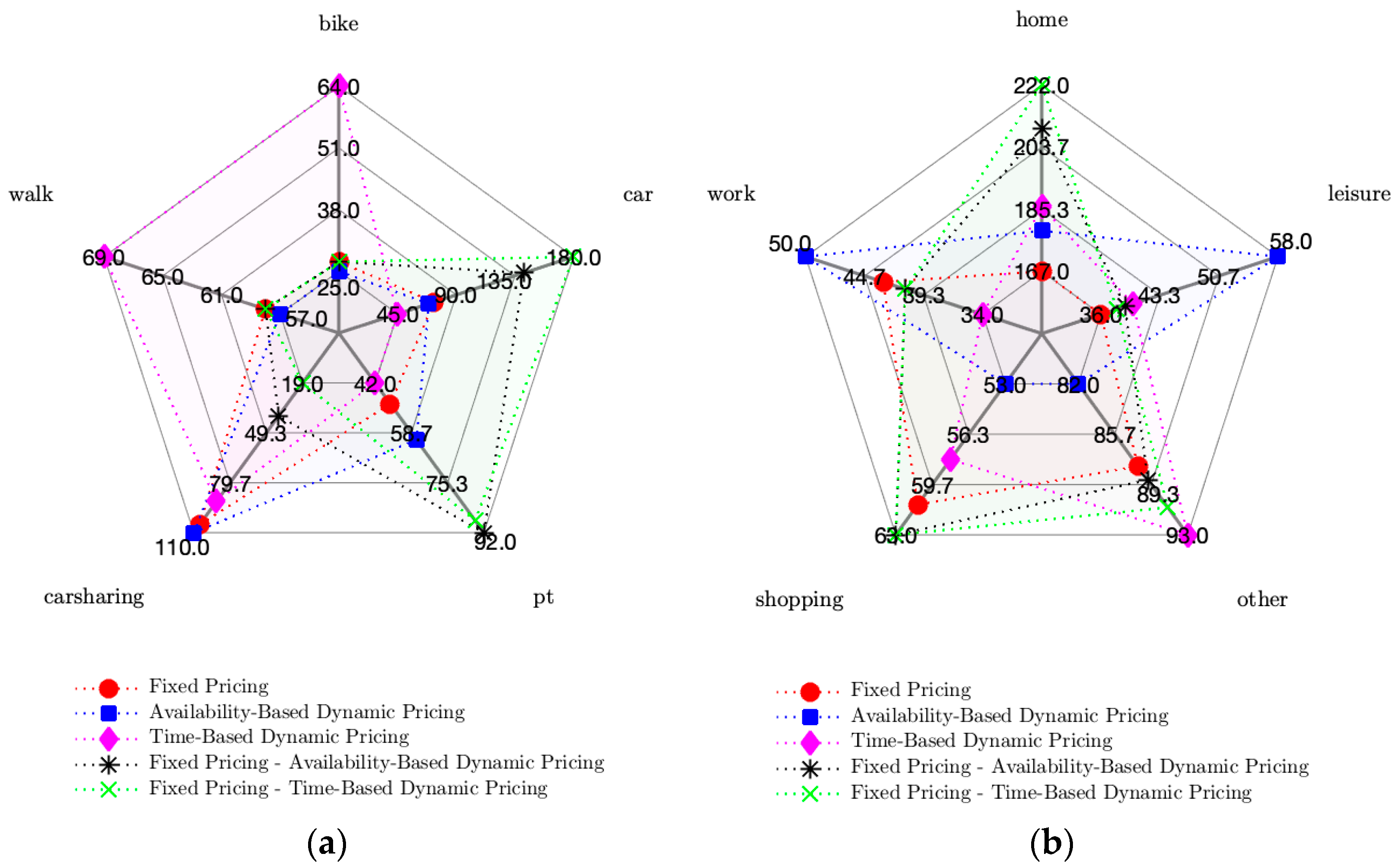
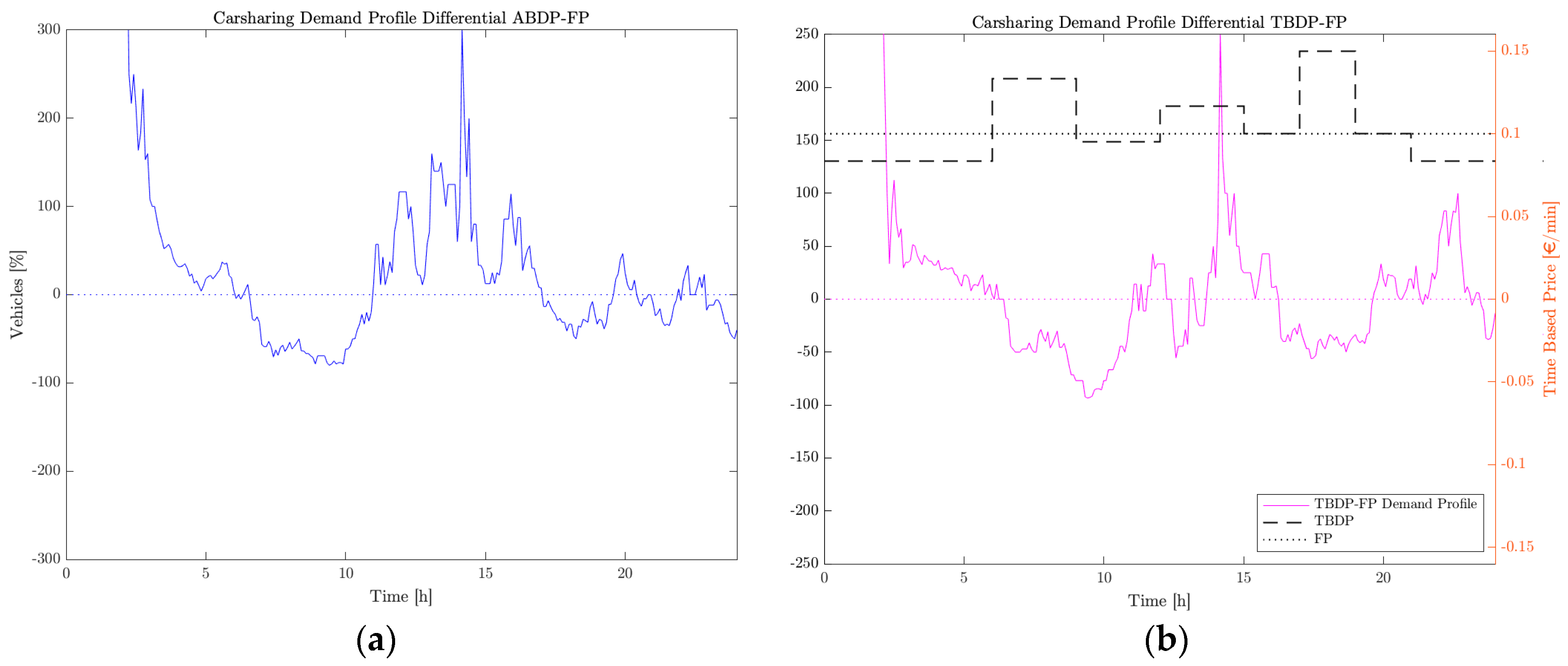
3.2. Effects on Demand for Radial Configuration (Scenario 1)
- FP-ABDP to the indicators retrieved in the ABDP simulation for the users that took the carsharing when a FP strategy was in place; and
- FP-TBDP to the indicators retrieved in the TBDP simulation for the users that took the carsharing when a FP strategy was in place.
3.3. Effects on Carsharing Operations for Coaxial Configuration (Scenario 2)
3.4. Effects on Demand for Coaxial Configuration (Scenario 2)
4. Discussion
5. Conclusions
Author Contributions
Funding
Acknowledgments
Conflicts of Interest
Appendix A
References
- Shaheen, S.; Sperling, D.; Wagner, C. A short history of carsharing in the 90′s. J. World Transp. Policy Pract. 1999, 5, 24. [Google Scholar]
- Cici, B.; Markopoulou, A.; Frias-Martinez, E.; Laoutaris, N. Assessing the potential of ride-sharing using mobile and social data: A tale of four cities. In Proceedings of the UbiComp 2014—ACM International Joint Conference on Pervasive and Ubiquitous Computing, Seattle, WA, USA, 13–17 September 2014; pp. 201–211. [Google Scholar]
- Schuster, T.D.; Byrne, J.; Corbett, J.; Schreuder, Y. Assessing the potential extent of carsharing a new method and its implications. Transp. Res. Rec. 2005, 1927, 174–181. [Google Scholar] [CrossRef]
- Burns, L.D. A vision of our transport future. Nature 2013, 497, 181–182. [Google Scholar] [CrossRef] [PubMed]
- Nijland, H.; van Meerkerk, J. Mobility and environmental impacts of car sharing in the Netherlands. Environ. Innov. Soc. Transit. 2017, 23, 84–91. [Google Scholar] [CrossRef]
- Martin, E.W.; Shaheen, S.A. Greenhouse gas emission impacts of carsharing in north America. IEEE Trans. Intell. Transp. Syst. 2011, 12, 1074–1086. [Google Scholar] [CrossRef]
- Shaheen, S. Shared mobility policy briefs: Definitions, impacts, and recommendations. Transp. Sustain. Res. Center 2018. [Google Scholar] [CrossRef]
- Degirmenci, K.; Breitner, M.H. Carsharing: A literature review and a perspective for information systems research. In Proceedings of the Tagungsband Multikonferenz Wirtschaftsinformatik, Paderborn, Germany, 26–28 February 2014; pp. 962–979. [Google Scholar]
- Perboli, G.; Ferrero, F.; Musso, S.; Vesco, A. Business models and tariff simulation in car-sharing services. Transp. Res. Part Policy Pract. 2018, 115, 32–48. [Google Scholar] [CrossRef]
- Di Febbraro, A.; Sacco, N.; Saeednia, M. One-way carsharing: Solving the relocation problem. Transp. Res. Rec. J. Transp. Res. Board 2012, 2319, 113–120. [Google Scholar] [CrossRef]
- Pfrommer, J.; Warrington, J.; Schildbach, G.; Morari, M. Dynamic vehicle redistribution and online price incentives in shared mobility systems. IEEE Trans. Intell. Transp. Syst. 2014, 15, 1567–1578. [Google Scholar] [CrossRef]
- Zhou, S. Dynamic Incentive Scheme for Rental Vehicle Fleet Management. Master’s Thesis, Massachusetts Intitute of Technology, Cambridge, MA, USA, 2012. [Google Scholar]
- Jorge, D.; Molnar, G.; de Almeida Correia, G.H. Trip pricing of one-way station-based carsharing networks with zone and time of day price variations. Transp. Res. Part B Methodol. 2015, 81, 461–482. [Google Scholar] [CrossRef]
- Brendel, A.B.; Zapadka, P.; Brennecke, J.T.; Kolbe, L.M. A decision support system for computation of carsharing pricing areas and its influence on vehicle distribution. In Proceedings of the ICIS 2017: Transforming Society with Digital Innovation, Seoul, Korea, 10–13 December 2017. [Google Scholar]
- Ciari, F.; Balac, M.; Balmer, M. Modelling the effect of different pricing schemes on free-floating carsharing travel demand: A test case for Zurich, Switzerland. Transportation 2015, 42, 413–433. [Google Scholar] [CrossRef]
- Harms, S.; Truffe, B. The Emergence of a Nation-Wide Carsharing Co-Operative in Switzerland; EAWAG: Zürich, Switzerland, 1998. [Google Scholar]
- Rieser, M. Researching the influence of time-dependent tolls with a multi-agent traffic simulation. In Proceedings of the European Transport Conference, Leiden, The Netherlands, 17–19 October 2007. [Google Scholar]
- Horni, A.; Nagel, K.; Axhausen, K.W. The Multi-Agent Transport Simulation MATSim; Ubiquity Press: London, UK, 2016. [Google Scholar]
- Horni, A.; Axhausen, K.W. Distribution of benefits and losses from roadpricing illustrated in a microsimulation scenario. Arb. Verk. Und Raumplan. 2014, 31, 974. [Google Scholar]
- de Freitas, L.M.; Schuemperlin, O.; Balać, M. Road pricing: An analysis of equity effects with MATSim. In Proceedings of the 16th Swiss Transport Research Conference, Ascona, Switzerland, 18–20 May 2016. [Google Scholar]
- Balac, M.; Ciari, F.; Axhausen, K.W. Modeling the impact of parking price policy on free-floating carsharing: Case study for Zurich, Switzerland. Transp. Res. Part C Emerg. Technol. 2017, 77, 207–225. [Google Scholar] [CrossRef]
- Kamatani, T.; Nakata, Y.; Arai, S. Dynamic pricing method to maximize utilization of one-way car sharing service. In Proceedings of the 2019 IEEE International Conference on Agents (ICA), Jinan, China, 18–21 October 2019; pp. 65–68. [Google Scholar]
- Zhang, J.; Meng, M.; Wang, D.Z.W. A dynamic pricing scheme with negative prices in dockless bike sharing systems. Transp. Res. Part B Methodol. 2019, 127, 201–224. [Google Scholar] [CrossRef]
- McAfee, R.P. Dynamic pricing in the airline industry. In Handbook on Economics and Information Systems; Elsevier: Amsterdam, The Netherlands, 2006; Volume 44. [Google Scholar]
- Williams, K.R. Dynamic airline pricing and seat availability. SSRN Electron. J. 2017, 2103. [Google Scholar] [CrossRef]
- Gibbs, C.; Guttentag, D.; Gretzel, U.; Yao, L.; Morton, J. Use of dynamic pricing strategies by Airbnb hosts. Int. J. Contemp. Hosp. Manag. 2018, 30, 2–20. [Google Scholar] [CrossRef]
- Giorgione, G.; Ciari, F.; Viti, F. Availability-based dynamic pricing on a round-trip carsharing service: An explorative analysis using agent-based simulation. Procedia Comput. Sci. 2019, 151, 248–255. [Google Scholar] [CrossRef]
- Du Plessis, W.; Joubert, J.W. Evaluating the effect of road pricing strategies in matsim, using agent-specific and income-dependent values. In Proceedings of the International Conference on Computers and Industrial Engineering, CIE 2012, Cape Town, South Africa, 16 July 2012; Volume 1, pp. 525–532. [Google Scholar]
- Cascetta, E. Transportation Systems Analysis: Models and Applications; Springer: Berlin/Heidelberg, Germany, 2009. [Google Scholar]
- Ciari, F.; Bock, B.; Balmer, M. Modeling station-based and free-floating carsharing demand: Test case study for Berlin. Transp. Res. Rec. 2014, 2416, 37–47. [Google Scholar] [CrossRef]
- Ciari, F.; Balmer, M.; Axhausen, K.W. Concepts for a Large Scale Car-Sharing System: Modeling and Evaluation with an Agent-Based Approach; Eidgenössische Technische Hochschule, Institut für Verkehrsplanung und Transportsysteme: Zurich, Switzerland, 2008. [Google Scholar]
- Lopes, M.M.; Martinez, L.M.; Correia, G.H.D.A. Simulating carsharing operations through agent-based modelling: An application to the city of Lisbon, Portugal. Transp. Res. Procedia 2014, 3, 828–837. [Google Scholar] [CrossRef]
- Laarabi, H.M.; Boldrini, C.; Bruno, R.; Porter, H.; Davidson, P. On the performance of a one-way car sharing system in suburban areas: A real-world use case. In Proceedings of the VEHITS 2017—3rd International Conference on Vehicle Technology and Intelligent Transport Systems, Porto, Portugal, 22 April 2017; pp. 102–110. [Google Scholar]
- Lu, Y.; Basak, K.; Carrion, C.; Loganathan, H.; Adnan, M.; Pereira, F.C.; Saber, V.H.; Ben-Akiva, M. SimMobility mid-term simulator: A state of the art integrated agent based demand and supply model. In Proceedings of the 94th Annual Meeting of the Transportation Research Board, Washington, DC, USA, 11–15 January 2015. [Google Scholar]
- PTV Group. PTV Evaluate Business Models for the Future of Mobility. Available online: //www.ptvgroup.com/en/mobilitynext/ (accessed on 8 January 2019).
- Burghout, W.; Koutsopoulos, H.N. Hybrid traffic simulation models: Vehicle loading at Meso-Micro Boundaries. In Transport Simulation; Chung, E., Dumont, A.-G., Eds.; EPFL Press: Lausanne, Switzerland, 2019; pp. 27–41. ISBN 978-0-429-09325-8. [Google Scholar]
- Wilensky, U.; Rand, W. An Introduction to Agent-Based Modeling: Modeling Natural, Social, and Engineered Complex Systems with NetLogo; MIT Press: Cambridge, MA, USA, 2015. [Google Scholar]
- Gatta, V.; Marcucci, E.; Pira, M.L.; Inturri, G.; Ignaccolo, M.; Pluchino, A. E-groceries and urban freight: Investigating purchasing habits, peer influence and behaviour change via a discrete choice/agent-based modelling approach. Transp. Res. Procedia 2020, 46, 133–140. [Google Scholar] [CrossRef]
- Nico Kühnel Network Editor for JOSM. Manual. Available online: https://josm.openstreetmap.de (accessed on 21 May 2020).
- Ziemke, D.; Nagel, K. Development of a Fully Synthetic and Open Scenario for Agent-Based Transport Simulations—The MATSim Open Berlin Scenario. Available online: https://svn.vsp.tu-berlin.de/repos/public-svn/publications/vspwp/2017/17-12/ZiemkeNagel2017BerlinScenario.pdf (accessed on 1 August 2019).
- Rieser, M.; Nagel, K.; Beuck, U.; Balmer, M.; Rümenapp, J. Agent-oriented coupling of activity-based demand generation with multiagent traffic simulation. Transp. Res. Rec. 2007, 2021, 10–17. [Google Scholar] [CrossRef]
- Amt für Statistik Berlin-Brandenburg. Available online: https://www.statistik-berlin-brandenburg.de/ (accessed on 1 August 2019).
- Axhausen, K.W.; Ehreke, I.; Glemser, A.; Hess, S.; Jödden, C.; Nagel, K. Schlussbericht: FE-Projekt-Nr. 96.996/2011; ETH: Zurich, Switzerland, 2015; p. 308. [Google Scholar]
- Ciari, F.; Schuessler, N.; Axhausen, K.W. Estimation of carsharing demand using an activity-based microsimulation approach: Model discussion and some results. Int. J. Sustain. Transp. 2013, 7, 70–84. [Google Scholar] [CrossRef]
- Martínez, L.M.; de Correia, G.H.A.; Moura, F.; Lopes, M.M. Insights into carsharing demand dynamics: Outputs of an agent-based model application to Lisbon, Portugal. Int. J. Sustain. Transp. 2017, 11, 148–159. [Google Scholar] [CrossRef]
- Berlin Traffic Report. TomTom Traffic Index. Available online: https://www.tomtom.com/en_gb/traffic-index/berlin-traffic/ (accessed on 4 August 2020).
- Geofabrik Berlin OSM. Available online: http://download.geofabrik.de/europe/germany/berlin.html (accessed on 21 May 2020).
- Welcome to the QGIS Project! Available online: https://www.qgis.org/en/site/ (accessed on 21 May 2020).
- Einwohnerinnen und Einwohner im Land Berlin am 31. December 2019. Available online: https://www.statistik-berlin-brandenburg.de/publikationen/stat_berichte/2020/SB_A01-05-00_2019h02_BE.pdf (accessed on 21 May 2020).
- Varrette, S.; Bouvry, P.; Cartiaux, H.; Georgatos, F. Management of an academic HPC cluster: The UL experience. In Proceedings of the 2014 International Conference on High Performance Computing & Simulation (HPCS), Bologna, Italy, 21–25 July 2014; IEEE: Bologna, Italy, 2014; pp. 959–967. [Google Scholar]
- Bösch, P.M.; Becker, F.; Becker, H.; Axhausen, K.W. Cost-based analysis of autonomous mobility services. Transp. Policy 2018, 64, 76–91. [Google Scholar] [CrossRef]


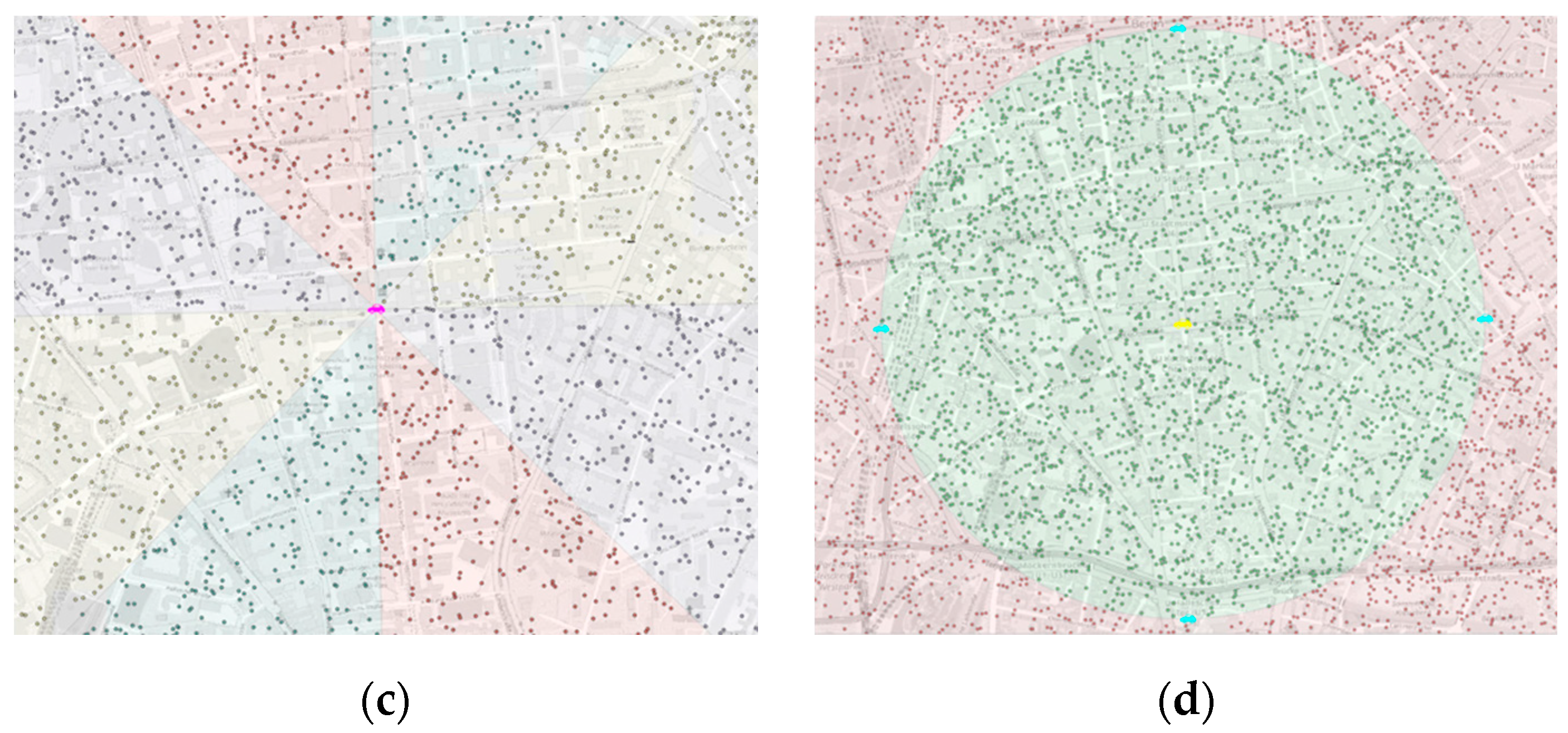
| Sector Name | VOT [€/h] | Stations Name | Color Code |
|---|---|---|---|
| Green | 4.00 | Central | Magenta |
| Yellow | 3.00 | Border | Orange |
| Purple | 2.00 | Inner | Cyan |
| Red | 0.50 |
| Sector Name | VOT [€/h] | Stations Name | Color Code |
|---|---|---|---|
| Green | 4.00 | Zone 4 | Yellow |
| Red | 3.00 | Zone 4–3 | Cyan |
| Cyan | 2.00 | Zone 3–2 | Blue |
| Grey | 0.50 | Zone 2–0.5 | Cyan |
| Zone 0.5 | Magenta |
| VOT [€/h] | Radial | Coaxial |
|---|---|---|
| 4.00 | 9959 | 2739 |
| 3.00 | 9987 | 4106 |
| 2.00 | 10,990 | 7310 |
| 0.50 | 8820 | 14,181 |
| Scenario Code | Name | Pricing Strategies | Color Code | |
|---|---|---|---|---|
| 1 | Radial configuration | Fixed |  |  |
| Availability-based |  | |||
| Time-based |  | |||
| 2 | Coaxial configuration | Fixed | |  |
| Availability-based | | |||
| Time-based | |
© 2020 by the authors. Licensee MDPI, Basel, Switzerland. This article is an open access article distributed under the terms and conditions of the Creative Commons Attribution (CC BY) license (http://creativecommons.org/licenses/by/4.0/).
Share and Cite
Giorgione, G.; Ciari, F.; Viti, F. Dynamic Pricing on Round-Trip Carsharing Services: Travel Behavior and Equity Impact Analysis through an Agent-Based Simulation. Sustainability 2020, 12, 6727. https://doi.org/10.3390/su12176727
Giorgione G, Ciari F, Viti F. Dynamic Pricing on Round-Trip Carsharing Services: Travel Behavior and Equity Impact Analysis through an Agent-Based Simulation. Sustainability. 2020; 12(17):6727. https://doi.org/10.3390/su12176727
Chicago/Turabian StyleGiorgione, Giulio, Francesco Ciari, and Francesco Viti. 2020. "Dynamic Pricing on Round-Trip Carsharing Services: Travel Behavior and Equity Impact Analysis through an Agent-Based Simulation" Sustainability 12, no. 17: 6727. https://doi.org/10.3390/su12176727
APA StyleGiorgione, G., Ciari, F., & Viti, F. (2020). Dynamic Pricing on Round-Trip Carsharing Services: Travel Behavior and Equity Impact Analysis through an Agent-Based Simulation. Sustainability, 12(17), 6727. https://doi.org/10.3390/su12176727