Article

Assessment of Groundwater Recharge in Agro-Urban Watersheds Using Integrated SWAT-MODFLOW Model

1
Department of Land, Water and Environment Research, Korea Institute of Civil Engineering and Building Technology, Goyang 10223, Korea
2
Department of Civil and Environmental Engineering, University of Science and Technology, Daejeon 34113, Korea
*
Author to whom correspondence should be addressed.
Sustainability 2020, 12(16), 6593; https://doi.org/10.3390/su12166593
Submission received: 29 July 2020 / Revised: 10 August 2020 / Accepted: 11 August 2020 / Published: 14 August 2020
(This article belongs to the Section Environmental Sustainability and Applications)

Abstract

:
Numerical models are employed widely to evaluate the hydrological components of a watershed but, traditionally, watershed models simplify either surface or subsurface flow module. In this setup, as a bridge between groundwater and surface water regimes, aquifer recharge is the most affected segment of the water balance. Since the watershed processes are increasingly changed, the need for a comprehensive model with detailed conceptualizing capacity of both groundwater and surface water flow systems is growing. This work focuses on the spatiotemporal groundwater recharge assessment in gauged and ungauged agro-urban watersheds in South Korea using the updated SWAT-MODFLOW model, which integrates the Soil and Water Assessment Tool (SWAT2012) and Newton–Raphson formulation for Modular Finite Difference Groundwater Flow (MODFLOW-NWT) in a single executable code. Before coupling, the setup, calibration, and verification of each model were performed separately. After integration, irrigation pumps and drain cells mapping to SWAT auto-irrigation and subbasins were initiated. Automatic calibration techniques were used for SWAT and MODFLOW-NWT models, but a manual calibration was used for the integrated model. A physical similarity approach was applied to transfer parameters to the ungauged watershed. Statistical model performance indicators revealed that the low streamflow estimation was improved in SWAT-MODFLOW. The spatiotemporal aquifer recharge distribution from both the stream seepage and precipitation showed a substantial change, and most of the aquifer recharge occurs in July–September. The areal annual average recharge reaches about 18% of the precipitation. Low-lying areas receive higher recharge consistently throughout a year. Overall, SWAT-MODFLOW exhibited reasonable versatility in evaluating watershed processes and produced valuable results with reasonable accuracy. The results can be an important input for policymakers in the development of sustainable groundwater protection and abstraction strategies for the region.

1. Introduction

The growing demand for water supply and the undesirable impact on the resources entails efficient management and detailed comprehension of hydrological cycle components [1,2,3,4]. Particularly, watershed processes in agricultural and urban areas are significantly affected and need a deeper understanding.
Extensive agriculture, urbanization/industrialization, and climate change affect the quality, quantity, and spatiotemporal distribution of water resources [5,6,7,8]. Urban sprawl introduces major topographic and natural vegetation changes because of the construction and utility systems, which result in high surface runoff and new recharge mechanisms, such as leakage from water mains, sewer leakage, artificial recharge, and infiltration via paved surfaces [9,10]. These recharge mechanisms may upsurge the groundwater level in urban regions and contribute to the flooding events unless there is a substantial abstraction [8,9]. Nonetheless, most urban areas have overmuch groundwater abstraction wells. Agricultural activities affect the water resources differently from urbanization: the major hydrological processes are irrigation pumping, seepage from irrigation canals, and return flow from agriculture water. Irrigation pumping changes with the season, but in urban areas, the withdrawal is throughout the year. In a highly irrigated area, groundwater overexploitation is expected, but irrigation agriculture also has the potential to increase the groundwater level [11].
Assessment of groundwater recharge is essential to ensure the balance between recharge and abstraction of groundwater, to compute the groundwater contribution to streams, to assess groundwater vulnerability to pollution, and to get an insight about the effect of climate and land use/land cover (LULC) changes on the spatiotemporal distribution of recharge [12,13]. This can be accomplished by understanding and conceptualizing the sources and controlling factors. The sources of recharge include both natural and artificial phenomena. The main natural recharge sources are precipitation, adjacent aquifers, and surface water bodies. Human-induced sources related to agro-urban activities include water loss from irrigation fields, canals, water supply lines, sewers, drainage pipes, septic tanks, and overwatering of parks and gardens. Climate; vegetation; nature of the unsaturated zone, including flow mechanism and thickness; available groundwater volume; soil properties; geology; LULC; topography; and depth to the water table are the primary recharge regulating factors [14,15].
The conceptualization of the various recharge mechanisms and controlling elements in a watershed is a fundamental step in the groundwater recharge estimation processes. Depending on the recharge mechanisms, governing factors, availability of data, required precision level, and spatial and temporal scale of the study area, the estimation method can be selected [16], though the selection is not straightforward as each method has advantages and limitations [15,16]. Several groundwater recharge estimation techniques are available, including water balance, Darcian, tracer, and empirical methods [13,15,16,17,18]. Numerical (semi-distributed) and tracer methods are widely used techniques [9,19].
The intent to conceptualize the actual watershed processes makes numerical modeling advantageous for the assessment of scenarios, such as the impact of LULC and climate change on not equal hydrological components of water resources. However, since most of the watershed scale models are developed by simplifying either groundwater or surface water flow processes [5,20], the conceptualization of the continuous hydrological processes between the atmosphere, the surface, and subsurface environments necessitate interdisciplinary tools [21].
SWAT (Soil and Water Assessment Tool) [22] and MODFLOW (Modular Three-Dimensional Finite-Difference Ground-Water Flow Model) [23] are public domain codes extensively employed for the evaluation, development, and management of water resources—chiefly in agricultural watersheds [5,20,24]. MODFLOW is a spatially distributed and physically based groundwater flow model that simulates the hydraulic head and flow systems in a heterogeneous aquifer setup. SWAT—a semi-distributed and physically based large-scale watershed model—computes groundwater–surface water processes. However, the recent version of the SWAT model has low performance in a watershed where groundwater seepage is a significant constituent of streamflow, and MODFLOW is incomplete in conceptualizing surface water flow [25,26]. To bridge the fragmented cross-disciplinary details in the evaluation of system responses under different scenarios, SWAT and MODFLOW models may be coupled [4,18,24,27,28,29,30,31,32,33]. All different versions of these integrated models are recapitulated by Bailey et al. [24] and Chunn et al. [34].
The recently coupled model (SWAT-MODFLOW) has several advantages, such as publicly open code, availability of graphical interface, use of the Newton–Raphson formulation for Modular Finite Difference Groundwater Flow (MODFLOW-NWT) [35], and the capability to integrate SWAT and MODFLOW models regardless of their spatial coverage differences [24]. The model has been tested, updated, and compared with SWAT model performance, as well [20,26,36,37]. The SWAT-MODFLOW [24] previous applications and modifications are summarized here.
Taie Semiromi and Koch [36] used SWAT-MODFLOW to investigate groundwater–surface water interaction in a mountainous region with intermittent drainage network dominated arid, agricultural watershed, in Iran. Gao et al. [37] reported the application of SWAT-MODFLOW to estimate the surface water resources in the agricultural watershed of Big Sunflower River, USA. The model was also applied in west-central Alberta to assess the effect of climate change and groundwater extractions on groundwater–surface water interactions in an agricultural watershed [34]. The groundwater abstraction in SWAT-MODFLOW was compared with the abstraction in the SWAT model [25]. Recently the model is applied to study groundwater–surface water interaction in plains, Argentina [5].
SWAT-MODFLOW is modified to simulate groundwater–surface water interaction in large-scale agro-urban watersheds [20,26]. Linking codes between MODFLOW pumping cells with the SWAT model Hydrologic Response Units (HRUs) for combined groundwater–surface water or groundwater-dependent irrigation practices was one of the modifications. The SWAT auto-irrigation algorithms were also modified so that when surface water irrigation is not sufficient it will be supplemented with groundwater irrigation. Therefore, the SWAT-MODFLOW allows the transfer of irrigation groundwater pumping to irrigation area (linking MODFLOW pumping cells to SWAT HRUs) and MODFLOW drain cells to SWAT subbasins.
The coupled SWAT and MODFLOW model can adequately quantify the spatiotemporal distribution of surface runoff, evapotranspiration (ET), groundwater recharge and discharge, and groundwater level [20,24,38]. However, the application is in limited regions and objectives due to extensive data preparation and the complexity of the model [25,39]. The application is mainly in arid and semi-arid areas [20,24], and the authors tend to focus on aquifer–stream interaction. In this study, the updated SWAT-MODFLOW was employed to assess the spatiotemporal distribution of groundwater recharge in gauged and ungauged agro-urban watersheds. In conjunction with the main objective, this work explored the versatility of the SWAT-MODFLOW algorithms to conceptualize watershed processes, which have a high density of urban and irrigation groundwater abstraction wells in multiple watersheds characterized by humid climate, complex topography, and detail LULC and soil classes. One of the improvements of the current version of the SWAT-MODFLOW model over the previous versions is handling large-scale study areas with big data size, and, therefore, this study assessed this improvement as well. In sum, this comprehensive application of SWAT-MODFLOW scrutinized the flexibility of the model to conceptualize and compute complex watershed processes efficiently.
When the integrated model was applied, the SWAT code estimates the groundwater recharge, and the advantage of the integrated model in the recharge assessment seems not explicit. However, usually, the SWAT model needs to be calibrated extensively to reduce the gap between measured and computed data. In this process, the groundwater recharge and other water balance segments can be affected, principally in groundwater-dominated watersheds. Moreover, the SWAT model reportedly has low performance in low flow computation [40].

2. Materials and Methods

2.1. General Description of the Study Area

The study area is in the south of Seoul city, South Korea, and encompasses three watersheds, which drain to the Han River. Han River crosses Seoul city, and it is the fourth-longest river across the Korean peninsula. In the study area, the watersheds have a total area of approximately 376 km2 and cover most parts of Anyang, Gwacheon, and Seongnam cities. A limited part of Gunpo and Uiwang cities also lie in the study area. The region has a highly undulating topography with an altitude varying 11–598 m above sea level (Figure 1), and about 62% of the region has a slope below 20%. The geological nature of the watersheds is composed of mainly metamorphic rock, unconsolidated sedimentary deposits, intrusive igneous rock, and carbonated salt rock.
The climate is temperate with four seasons: winter, summer, spring, and autumn. The summer and winter have a significant temperature difference. The highest precipitation and humidity occur in a short period of summer (July–August). For the period of 2002–2018, the annual average humidity, precipitation, and minimum and maximum temperatures were about 69%, 1397 mm, and 8.5 and 17.5 °C, respectively. The streams are gauged for a lengthy period (starting before 2002) except the stream with an outlet labeled as SG4 (Figure 1). The streamflow gets its peak in summer and the rough in winter.
The land use in the study area is predominantly urban and agriculture. The urban-industrial landscape covers about 27% of the total area, and agricultural activities cover 13%. Overgrown dominate the mountainous topography, whereas the low-lying areas are residential. The forest coverage of the area, including range bushes, reaches up to 54%, and the rest of the area (6%) is covered by wetlands, water bodies, grasslands, and others. In the SWAT model-based classification, the LULC has 21 classes (Figure 2).
Figure 3 provides the soil type and hydrological soil groups in the study area. The soil types, SWAT code-based classes, are 115. Most of the soil types have four layers, and the maximum depth varies 130–2200 mm. Soils with “A”-type hydrologic soil group, which represents sand and sandy loam soil texture with low runoff potential, dominate (64.2%) the region, followed by group “B” (28%). Hydrologic soil group “B” encompasses loam and silt loam soils; this group has a moderate infiltration rate. Group “C” includes sandy clay loam soils and “D” clay, clay loam, silt clay, and sand clay soils. Hydrologic soil group “C” covers about 2% and “D” 5.8%. Groups “C” and “D” have low infiltration and high runoff potentials and occupy predominantly the lowland area inclusive of wetlands and water bodies.
The nationally available data were collected from different sources. Soil and LULC data were collected from National Institute of Agricultural Sciences and the Ministry of Environment of Korea, respectively. The daily streamflow data were acquired from Water Resources Management Information System [42] and the weather data from Meteorological Agency Weather Data Service [43].

2.2. SWAT Model

In this study, the SWAT2012 (ver.636) model was employed. SWAT is a large area watershed model in which computation is based on HRUs and subbasin scales [44,45]. The HRU is the smallest structured element of the delineated watershed comprising a unique combination of soil, LULC, and landscape features in a subbasin. Fixing the optimal number of HRUs is an important step to optimize the model size without losing important information [46]. The SWAT model has multiple HRU definition options, but dominant LULC, soil, and slope option and multiple HRU options are the most extensively employed methods. In this study, we have explored both options. When the first option—dominant LULC, soils, and slope class—was used, limited data encompassed and produced HRUs equal to the number of subbasins. The second option can be done by fixing the threshold values depending on the required number of HRUs; zero threshold value uses full physiographic data and produces a large number of HRUs if the data have a large-scale. Since the data are in detail for the region, using the common 5–10% thresholds can cause the loss of considerable information, and thus we employed this option with zero threshold values.
The watersheds were delineated using a 30 m resolution digital elevation model (DEM) and divided into 29 subbasins. Then, by combining slope classes, soil, and LULC data, 9424 HRUs were created using zero threshold value (multiple HRU option). In the region, there are seven precipitation and two weather stations (Figure 1). Wind speed, precipitation, humidity, maximum–minimum temperature, and solar radiation data were imported and written. The SWAT model simulation was performed for 13 years (2006–2018). The first three of the simulations were a warmup period—the model does not give output for these years.
The SWAT model was calibrated and validated at three streamflow gauges using SWAT-CUP [47] on a daily time step. Fifteen parameters—selected from the initial simulation of the model for 500 times—were optimized. The parameters are groundwater (ALPHA_BF, RCHRG_DP, GWQMN, REVAPMN, and GW_REVAP), soil water (SOL_BD, SOL_K, and SOL_AWC), lateral flow (HRU_SLP), surface runoff (OV_N, SURLAG, and CN2), canopy storage (CANMX), evaporation (ESCO), and hydraulic conductivity of main channel (CH_K2). The same parameter settings were used for all the three watersheds. The descriptions and minimum–maximum value limits are summarized in Table 1.
The model performance is verified based on RSR (the ratio of root mean square error (RMSE) and standard deviation of observed data), Nash–Sutcliffe efficiency (NSE), and percentage bias (PBIAS) values [48]. Mathematically, the value of NSE varies from negative infinity to one, but a value greater than 0.5 is commonly endorsed. An NSE value closer to one implies the model results are considerably closer to the measured data. While zero is the ideal value for RSR and PBIAS, the recommended ranges are 0–0.7 and ±25, respectively. The negative value of PBIAS indicates overestimated model outputs. The regression coefficient (R2) is also used to depict how close the measured and computed data are to a 45-degree line. SWAT-CUP has multiple options for the objective function. In this work, NSE was set as the objective function in all the simulations of calibrations and validations.
The regionalization approach, information transfer technique from one watershed to another [49], was used to estimate the parameters for the ungauged watershed (subbasins 11, 18, 21, and 27). The arithmetic mean, spatial proximity, physical similarity, regression, and watershed-runoff response similarity approaches can be employed to transfer optimized parameters from gauged watersheds to ungauged watersheds [50]. In this study, since the number of watersheds is limited and the coverage area is not significant physical similarity approach was employed. The physical similarity technique uses watersheds’ properties—commonly LULC, soil classes, and topography—as descriptors. The soil, LULC, and slope features of subbasins compared with the SWAT’s HRU report table were used as an indicator of similarity. Accordingly, the watershed with outlet SG3 (see Figure 1) was the donor watershed.

2.3. MODFLOW Model

The groundwater flow model, which encompasses the three watersheds, was built using the MODFLOW package of GMS 10.0 (Groundwater Modeling System; Aquaveo). MODFLOW is a finite-difference model that solves the three-dimensional flow of groundwater through porous earth material [51]. Specifically, MODFLOW-NWT version 1.0.08 09/01/2013 [35], Newton–Raphson formulation for MODFLOW-2005 version 1.11.0 08/08/2013, was employed in this study. MODFLOW-NWT uses the upstream weighting (UPW) package and smooth storage changes during cell wetting/drying and transitions between confined and unconfined conditions. MODFLOW-NWT has profound advantages over MODFLOW-2005, which are simulating groundwater flow in an unconfined aquifer without changing dry cells to inactive cells and calculating hydraulic head for dry cells during the simulation [35]. The UPW package has the functionality to set the flow out of the dry cells to zero and calculates the groundwater head from the inflow to the dry cells.
The spatial extent of the groundwater flow model encloses the three watersheds. The model area was discretized into a 100 m × 100 m horizontal resolution. The discretized model area has 9768 active cells. The stream network generated using the SWAT model was imported to MODFLOW to create the stream cells; using the river package 1344 stream cells were identified. Limited water flow lines, which are not simulated as streams (see Figure 4), were represented as drain cells. The top elevation of the model was extracted from 30 m resolution DEM. The bottom boundary was interpolated from the field electrical resistivity test. The bottom elevation ranges 50–100 m below the surface.
Sources and sinks, initial head, riverbed conductance, and hydraulic conductivity were processed and incorporated into the model to simulate steady-state groundwater flow. The recharge was summarized from SWAT output in the subbasin-scale and imported to MODFLOW. The well package was used to incorporate the groundwater abstraction from 1745 wells with a pumping rate of 0.76–250 m3/day. Around 54% of groundwater abstraction is for agriculture use, and 46% is for domestic and industrial purposes. The initial head and hydraulic conductivity were interpolated from the field recorded head and pump test data (23 pumping test wells). In the region, there are 32 monitoring wells. Figure 4 presents the distribution of irrigation and industrial pumping wells, stream cells, and drain cells.
Since the initial simulation showed a difference in the measured and simulated head in most of the areas, the model was calibrated using Parameter ESTimation (PEST) algorithm by adding additional pilot points at data-scarce zones. The pilot point technique is flexible to estimate spatial variable parameters [52]. The calibration was performed systematically. Initially, the pilot points with the field pump test were locked; the parameter optimization was only at the added pilot points. Then, these pilot points were included in the calibration (unlocked), and the hydraulic conductivity was refined by fixing all the pilot points to the same minimum and maximum value of 0.001–26 m/day. The hydraulic conductivity obtained from the pumping test is in a range of 0.001–23.7 m/day. The riverbed conductance was also estimated during the calibration process in 0.001–31 m/day bounds. The calibration performance was evaluated based on RMSE and R2.
After a satisfactory match between measured and computed head was obtained in the steady-state simulation, the transient-state simulation setup was initiated. To consider the variation of irrigation pumping, the simulation time was classified into stress periods: three stress periods per year. The irrigation period in the study area lasts from April to the beginning of June. In the transient simulation, additional parameters, namely specific storage and specific yield, were set before proceeding to the SWAT and MODFLOW coupling procedure.

2.4. Integrated SWAT-MODFLOW Model

SWAT-MODFLOW [24] integrates SWAT2012 and MODFLOW-NWT, and the linking code enables the two models to share their computations on a daily basis without the need for rewriting and importing the model inputs. Most importantly, the SWAT’s groundwater function is replaced by the MODFLOW code in the integrated model. The coupling is based on geographically located HRUs (disaggregated HRU (DHRU)) and MODFLOW grid shapefile.
Currently, this model has two Python-based graphical interfaces, i.e., SWATMOD-Prep [53] and QSWATMOD [39] and two versions of executable codes (SWAT-MODFLOW3 and SWAT-MODFLOW8). Both interfaces can create a simple MODFLOW model or import an existing groundwater flow model and integrate it with the SWAT model. For this work, QSWATMOD with SWAT-MODFLOW3 (the latest version) was employed for its flexibility in giving geographical context with maps and post-processing of outputs. The basic producers and concepts are highlighted by Bailey et al. [24].
To perform the coupling, all the required inputs, namely subbasin, HRUs, and river network shapefiles and ‘textinout’ from the SWAT model and grid shapefile and MODFLOW model native text (‘nam’ file) from MODFLOW-NWT simulation need to be imported. Accordingly, moderately calibrated models and shapefiles imported and proceed to the coupling step. The stream network can either be from the MODFLOW or SWAT model. MODFLOW stream cells were selected to be used directly since the riverbed conductance went under modifications. Then, the HRUs disaggregated to DHRUs and coupled with the MODFLOW grid cells. Once the models were integrated, all the required linking files were created. The irrigation pumping and drain cells from MODFLOW model mapping were done in the model setup process, and the simulation was performed 2006–2018, including the first three years of warmup period. A manual calibration technique was used to optimize the principally specific storage, specific yield, and SWAT’s groundwater and surface water flow parameters (ALPHA_BF, OV_N, CN2, and CH_K2).
During the simulation, the computation exchange was on a daily basis. Deep percolation computed at the HRU-scale transferred to DHRUs and then mapped to MODFLOW grid cells to build the stress values in the recharge package. The aquifer–stream water flux computed using the river package of the MODFLOW model totaled to each subbasin. Finally, the SWAT’s routing algorithm ran to rout the computed runoff and groundwater discharge volume.

3. Results

This section discusses the models’ calibration and validation performance and principal water balance segments of the region. The degree of accuracy of computed results is highlighted based on commonly used statistical indicators and visual inspection from comparative graphs. Both SWAT and SWAT-MODFLOW model outputs are substantial, but groundwater recharge and stream–aquifer interaction are emphasized here, aligned with the objective.

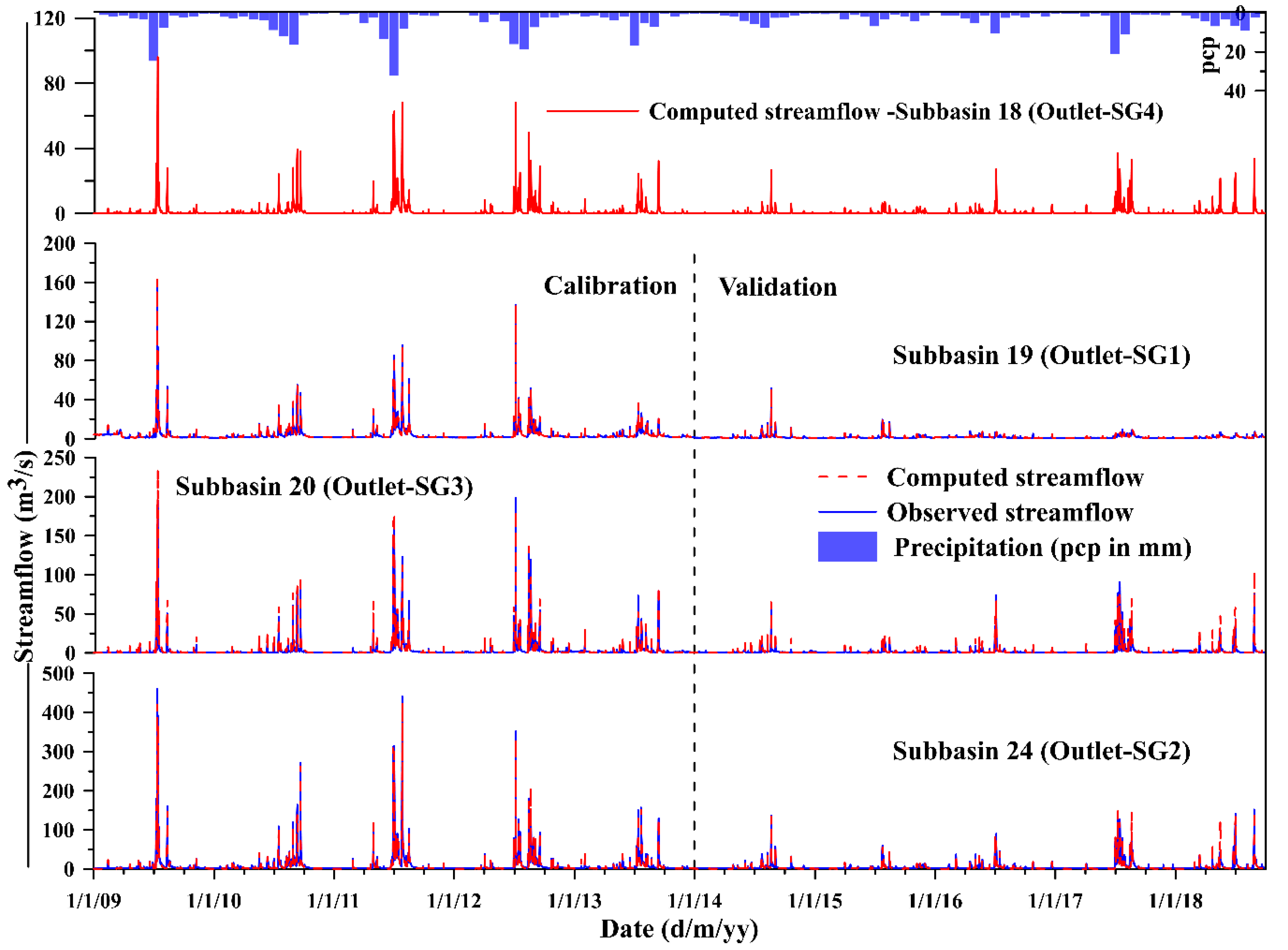
3.1. Model Calibration and Validation Performance

The calibration and verification of the models were performed in multiple stages. First, the SWAT and MODFLOW automatic calibrations and validation were undertaken to adjust the key parameters of each model separately. Then, the integrated model was calibrated manually. The accuracies of the outputs were weighed by observed data referenced comparison (Figure 5, Figure 6 and Figure 7).
The steady-state calibrated groundwater hydraulic head, presented in Figure 5, reflects the topographic complexity of the region. In the region, the hydraulic head reaches 10–212 m. While the middle and eastern part of the model has a high groundwater head, the low-lying areas have a low depth to the water table. The overall statistical and visual inspection of the model output depicts the observed and computed head match well except at the southeast of the region where relatively higher discrepancies were observed. Figure 5a shows the monitoring wells scaled on the calibration error of each well.
The SWAT model calibration (January 2009–December 2013) and validation (January 2014–September 2018) periods were selected based on the availability of daily streamflow recorded with no missed dates. The statistical model performance indicators and visual comparisons are presented in Table 2 and Figure 6. While NSE and RSR values prove the performance of the model is “very good” for all outlets, the PBIAS is “satisfactory” and “unsatisfactory”, based on the scales given by Moriasi et al. [48]. The model overestimated the streamflow in subbasin 20 and underestimated in subbasins 19 and 24. Since the difference between the model results evaluation statistical values is significant (e.g., NSE and PBIAS), we stopped enforcing the model further.
Specific storage and specific yield were adjusted after the model integration. The final calibrated parameters are 1 × 10⁻⁴ m−1 (specific storage) and 0.18 (specific yield). Compared to the SWAT model calibration results, the SWAT-MODFLOW got more improvement in PBIAS (Table 2). However, the observed and computed streamflow plot of the SWAT and SWAT-MODFLOW model do not show the change, and thus only the SWAT-MODFLOW output and measured streamflow is shown in Figure 6. The two watersheds’ flow is plotted in comparison with the measured data. Since the other watershed (outlet SG4) is ungauged, only the computed streamflow is shown. The computed streamflow in the ungauged watershed also reflects the seasonality and precipitation pattern of the area well.
Comparison of the SWAT and SWAT-MODFLOW simulations is not the focus here since the models are compared previously as discussed in the previous sections. Nevertheless, the highlighted model performance improvements reassert the preference to use SWAT-MODFLOW in groundwater flow dominated regions.
The head monitoring was performed May 2017–September 2018, but most of the monitoring wells do not have a continuous daily record. Therefore, 10 monitoring wells that have comparatively continuous measurements for a duration varying from three months to nearly a year were selected for calibration of the SWAT-MODFLOW model simulation. The graphical comparison of the model output and monitored data (Figure 7) exhibit a reasonable match. The maximum difference between measured and observed head is less than 1 m. The model captured the seasonal fluctuation of the hydraulic head well. Most of the monitoring wells show a maximum head change in April and May.

3.2. Principal Water Segments of the Region

In this section, first, monthly averages of the main water balance segments of the study area are summarized, and then the aquifer–stream interaction and the aquifer recharge are detailed. The principal water balance components of the region are presented in the form of water depth (in mm).
Figure 8 describes the major water balance components from the SWAT-MODFLOW model. The average groundwater pumping from MODFLOW for irrigation is 1.06 × 10⁴ m3/year, and 9.3% of it returns to the SWAT model per year. The basin annual average drain from the MODFLOW is around 4.67 mm. The annual average ET of the region is about 516 mm. The ET is high even though less evaporation is expected due to the urban coverage. In the area, the groundwater volume changes by 44.18 mm annually.

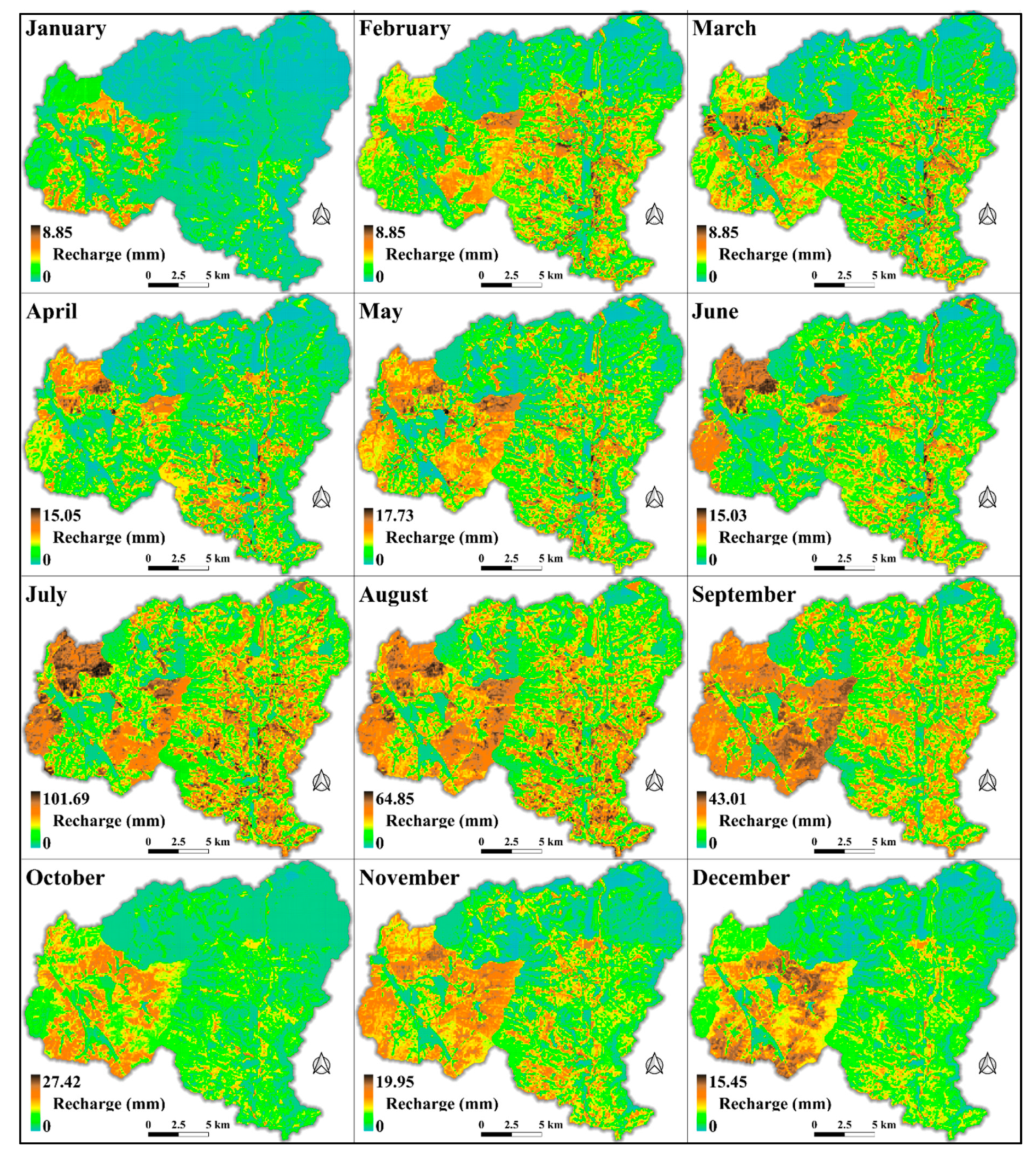
3.2.1. Groundwater Recharge

Figure 9 presents the average monthly groundwater recharge distribution. Even though the northeast and southwest of the region have a yearlong minimum and maximum recharge, respectively, spatially the recharge magnitude is intricately distributed and difficult to associate with the physiographic features of the region. This indicates that the aggregate of the spatial data is reflected in the model output rather than the separate entity data. Nevertheless, the lower elevation areas receive the maximum recharge of the month consistently.
Most of the region gets groundwater recharge yearlong. The maximum and large portion of the recharge occurs in July–September; in these months, the maximum recharge varies from 43.01 mm (September) to 101.69 mm (July). In the area, January–March are months of the lowest recharge; the highest value is 8.85 mm, and a substantial part of the region gains 0–1.5 mm recharge. The annual areal average recharge is about 18% of the precipitation.

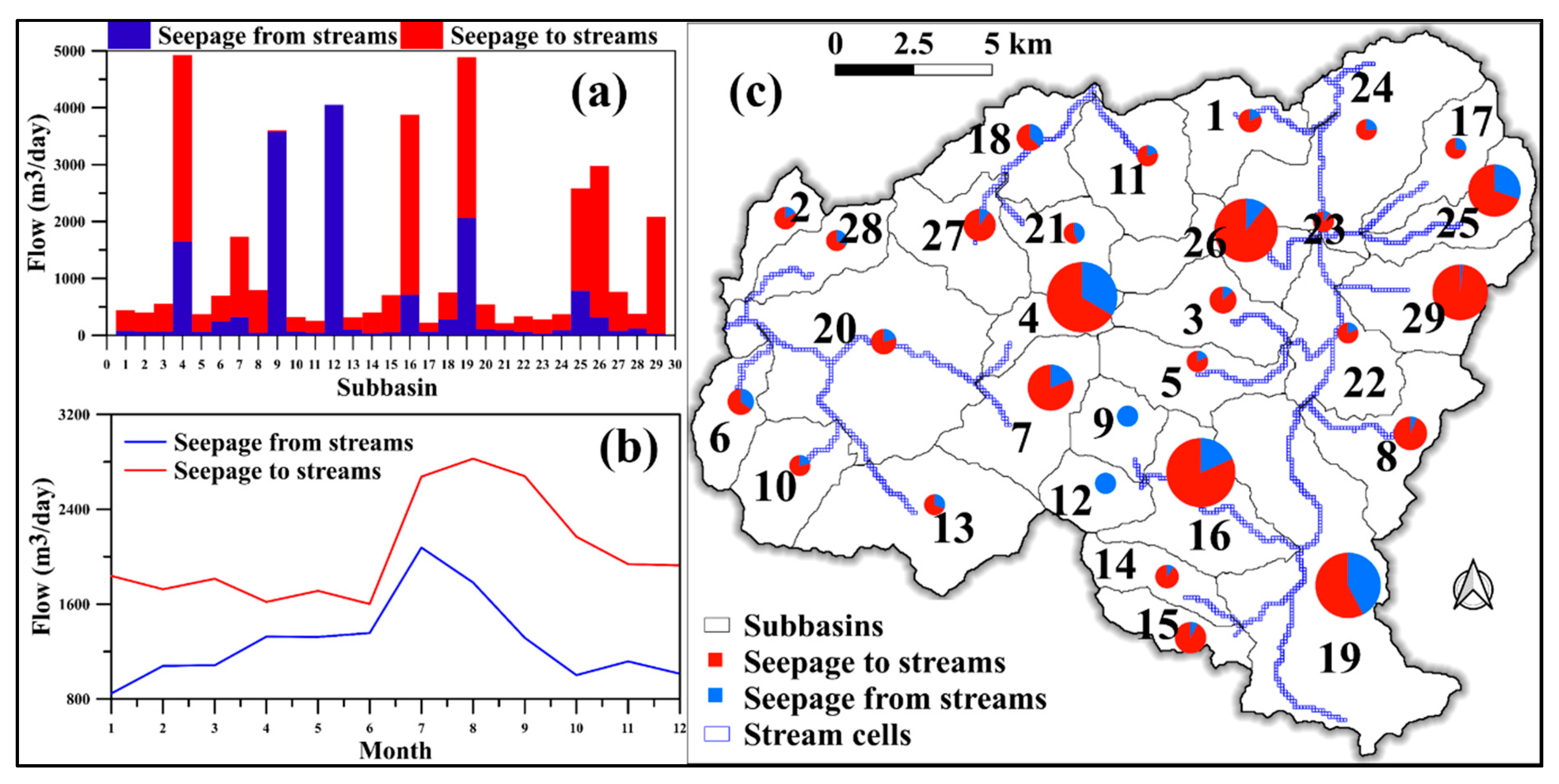
3.2.2. Stream–Aquifer Interaction

Stream–aquifer interaction is a vital part of the water balance components of a watershed, and understanding the spatiotemporal distribution is needed for efficient water resources management [3]. One of the principal reasons the SWAT-MODFLOW model was employed to assess the groundwater recharge in this study is the capability of the model to calculate the stream–aquifer interaction and so that the SWAT model calibration process can not affect the recharge magnitude significantly. SWAT-MODFLOW estimates the aquifer–stream interaction (seepage from stream to aquifer and seepage to streams from the aquifers) using Darcy’s law based on the river package of the MODFLOW model code. The package compares the groundwater hydraulic head with the water level in the stream cells to define the flow direction and estimate the magnitude of the flow. The interaction also depends on the riverbed conductance, precipitation events, and the hydraulic conductivity of the aquifer.
Figure 10 depicts the spatiotemporal distribution of stream–aquifer water exchange summarized in the subbasin-scale from stream cell scale output. The stream cell scale result shows the groundwater flow to streams is 1000–7480.4 m3/day in the wet months and 1000–5024.5 m3/day in dry months, whereas stream discharge to aquifers is 100–1294.3 m3/day and 100–404m3/day (Figure 10b). The subbasins summary reveals the spatial variability of the aquifer–stream interaction. Most of the seepage from stream cells is in subbasins 9 and 12; in these subbasins, the seepage to streams is negligible. The maximum groundwater seepage to streams takes place in subbasins 4, 16, and 19, and proportionally in subbasin 29, the sizeable portion is seepage to stream cells. The highest magnitude of stream–aquifer interaction occurs in July–August.
In most of the subbasins, the maximum water flow to streams develops at the starting point of streams. The result reveals that streams and aquifers are fully connected: there is water exchange almost in all stream cells.

4. Summary and Conclusions

The newly integrated SWAT-MODFLOW model was employed to study the groundwater recharge in gauged and ungauged agro-urban watersheds. The basic model setup, parameter optimization, and verification of the SWAT and MODFLOW model were performed before the coupling of the two models. The integrated model calibration was accomplished manually by comparing the observed hydraulic head and streamflow. For the ungauged watershed, the SWAT model parameters were transferred using the physical similarity technique. The SWAT-MODFLOW model performance was evaluated on both streamflow and groundwater levels and indicated improved performance in streamflow simulation compared to the SWAT model, particularly in PBIAS. The integrated model enabled the conceptualization of a variety of hydrological processes, including groundwater pumping (for irrigation and other uses), seepage from/to surface water bodies, and ET. The water balance components of the region were evaluated principally in terms of groundwater recharge and discharge, ET, surface runoff, lateral flow, and soil water. The stream–aquifer water exchange occurs in almost all stream cells: the two systems are fully connected in the study area. The long-term average groundwater recharge showed substantial spatiotemporal variations. The low-lying region receives higher recharge throughout the year, and the maximum recharge occurs July–September. Interestingly, the result showed that the area has high ET despite the large urban area coverage. In sum, this study presented the application and performance of the SWAT-MODFLOW model in a region characterized by a humid climate, shallow depth to the groundwater table, diversified hydrological processes, detailed physiographic data which resulted in big model size (9424 HRUs and 100 m × 100 m MODFLOW grid size), and complex topography. The model has a promising direction for assessment of the watershed process in areas with similar stresses and environmental conditions. The model outputs provide an important insight into principally the spatiotemporal distribution of groundwater recharge, under the agro-urban environment, in the study area. The results are comprehensive and can be used for planning, reassessing permissible groundwater abstraction rates, and protecting high groundwater recharge areas to achieve sustainable groundwater resource development and water resource management. Moreover, the results will be a reference for future changes in the water balance components resulted from recharge altering agro-urban activities.

Author Contributions

Conceptualization and methodology, B.A.Y. and I.-M.C.; validation, B.A.Y.; investigation, B.A.Y. and M.-G.K.; resources and data curation, I.-M.C. and M.-G.K.; writing—original draft preparation, B.A.Y.; writing—review and editing, B.A.Y. and I.-M.C.; visualization, B.A.Y.; supervision, I.-M.C. and S.W.C.; project administration, I.-M.C.; funding acquisition, I.-M.C. All authors have read and agreed to the published version of the manuscript.

Funding

This study was funded by the Korea Ministry of Environment (MOE) as a Demand Responsive Water Supply Service Program (146515).

Conflicts of Interest

The authors declare no conflict of interest.

References

  1. Fleckenstein, J.H.; Krause, S.; Hannah, D.M.; Boano, F. Groundwater-surface water interactions: New methods and models to improve understanding of processes and dynamics. Adv. Water Resour. 2010, 33, 1291–1295. [Google Scholar] [CrossRef]
  2. Winter, T.C.; Harvey, J.W.; Franke, O.L.; Alley, W.M. Ground Water and Surface Water—A Single Resource—U.S. Geological Survey Circular 1139; U.S. Geological Survey: Denver, CO, USA, 1998. [Google Scholar]
  3. Sophocleous, M. Interactions between groundwater and surface water: The state of the science. Hydrogeol. J. 2002, 10, 52–67. [Google Scholar] [CrossRef]
  4. Sophocleous, M.A.; Koelliker, J.K.; Govindaraju, R.S.; Birdie, T.; Ramireddygari, S.R.; Perkins, S.P. Integrated numerical modeling for basin-wide water management: The case of the Rattlesnake Creek basin in south-central Kansas. J. Hydrol. 1999, 214, 179–196. [Google Scholar] [CrossRef]
  5. Guevara Ochoa, C.; Medina Sierra, A.; Vives, L.; Zimmermann, E.; Bailey, R. Spatio-temporal patterns of the interaction between groundwater and surface water in plains. Hydrol. Process. 2020, 34, 1371–1392. [Google Scholar] [CrossRef]
  6. Jolly, I.D.; McEwan, K.L.; Holland, K.L. A review of groundwater-surface water interactions in arid/semi-arid wetlands and the consequences of salinity for wetland ecology. Ecohydrology 2008, 1, 43–58. [Google Scholar] [CrossRef]
  7. Kalbus, E.; Reinstorf, F.; Schirmer, M. Measuring methods for groundwater-surface water interactions: A review. Hydrol. Earth Syst. Sci 2006, 10, 873–887. [Google Scholar] [CrossRef] [Green Version]
  8. Sharp, J.M. The impacts of urbanization on groundwater systems and recharge. Aquamundi 2010, 1, 51–56. [Google Scholar] [CrossRef]
  9. Hamel, P.; Daly, E.; Fletcher, T.D. Source-control stormwater management for mitigating the impacts of urbanisation on baseflow: A review. J. Hydrol. 2013, 485, 201–211. [Google Scholar] [CrossRef]
  10. Salvadore, E.; Bronders, J.; Batelaan, O. Hydrological modelling of urbanized catchments: A review and future directions. J. Hydrol. 2015, 529, 62–81. [Google Scholar] [CrossRef]
  11. Meredith, E.; Blais, N. Quantifying irrigation recharge sources using groundwater modeling. Agric. Water Manag. 2019, 214, 9–16. [Google Scholar] [CrossRef]
  12. Götzinger, J.; Barthel, R.; Jagelke, J.; Bárdossy, A. The role of groundwater recharge and baseflow in integrated models. Iahs-Aish Publ. 321 2008, 103–109. [Google Scholar] [CrossRef]
  13. Zomlot, Z.; Verbeiren, B.; Huysmans, M.; Batelaan, O. Spatial distribution of groundwater recharge and base flow: Assessment of controlling factors. J. Hydrol. Reg. Stud. 2015, 4, 349–368. [Google Scholar] [CrossRef] [Green Version]
  14. Sanford, W. Recharge and groundwater models: An overview. Hydrogeol. J. 2002, 10, 110–120. [Google Scholar] [CrossRef]
  15. Walker, D.; Parkin, G.; Schmitter, P.; Gowing, J.; Tilahun, S.A.; Haile, A.T.; Yimam, A.Y. Insights From a Multi-Method Recharge Estimation Comparison Study. Groundwater 2018. [Google Scholar] [CrossRef] [Green Version]
  16. Scanlon, B.R.; Healy, R.W.; Cook, P.G. Choosing appropriate techniques for quantifying groundwater recharge. Hydrogeol. J. 2002, 10, 18–39. [Google Scholar] [CrossRef]
  17. De Vries, J.J.; Simmers, I. Groundwater recharge: An overview of processes and challenges. Hydrogeol. J. 2002, 10, 5–17. [Google Scholar] [CrossRef]
  18. Chung, I.-M.; Kim, N.-W.; Lee, J.; Sophocleous, M. Assessing distributed groundwater recharge rate using integrated surface water-groundwater modelling: Application to Mihocheon watershed, South Korea. Hydrogeol. J. 2010, 18, 1253–1264. [Google Scholar] [CrossRef]
  19. Ebrahimi, H.; Ghazavi, R.; Karimi, H. Estimation of Groundwater Recharge from the Rainfall and Irrigation in an Arid Environment Using Inverse Modeling Approach and RS. Water Resour. Manag. 2016, 30, 1939–1951. [Google Scholar] [CrossRef]
  20. Aliyari, F.; Bailey, R.T.; Tasdighi, A.; Dozier, A.; Arabi, M.; Zeiler, K. Coupled SWAT-MODFLOW model for large-scale mixed agro-urban river basins. Environ. Model. Softw. 2019, 115, 200–210. [Google Scholar] [CrossRef]
  21. Furman, A. Modeling Coupled Surface-Subsurface Flow Processes: A Review. Vadose Zone J. 2008, 7, 741–756. [Google Scholar] [CrossRef] [Green Version]
  22. Arnold, J.G.; Srinivasan, R.; Muttiah, R.S.; Williams, J.R. LARGE AREA HYDROLOGIC MODELING AND ASSESSMENT PART I: MODEL DEVELOPMENT. J. Am. Water Resour. Assoc. 1998, 34, 73–89. [Google Scholar] [CrossRef]
  23. McDonald, M.; Harbaugh, A.W. A Modular Three-Dimensional Finite-Difference Ground-Water Flow Model; U.S. Geological Survey: Reston, WV, USA, 1988. [Google Scholar]
  24. Bailey, R.T.; Wible, T.C.; Arabi, M.; Records, R.M.; Ditty, J. Assessing regional-scale spatio-temporal patterns of groundwater–surface water interactions using a coupled SWAT-MODFLOW model. Hydrol. Process. 2016, 30, 4420–4433. [Google Scholar] [CrossRef]
  25. Molina-Navarro, E.; Bailey, R.T.; Andersen, H.E.; Thodsen, H.; Nielsen, A.; Park, S.; Jensen, J.S.; Jensen, J.B.; Trolle, D. Comparison of abstraction scenarios simulated by SWAT and SWAT-MODFLOW. Hydrol. Sci. J. 2019, 64, 434–454. [Google Scholar] [CrossRef]
  26. Wei, X.; Bailey, R.T. Assessment of System Responses in Intensively Irrigated Stream–Aquifer Systems Using SWAT-MODFLOW. Water 2019, 11, 1576. [Google Scholar] [CrossRef] [Green Version]
  27. Menking, K.M.; Syed, K.H.; Anderson, R.Y.; Shafike, N.G.; Arnold, J.G. Model estimates of runoff in the closed, semiarid Estancia basin, central New Mexico, USA. Hydrol. Sci. J. 2003, 48, 953–970. [Google Scholar] [CrossRef]
  28. Kim, N.W.; Chung, I.M.; Won, Y.S.; Arnold, J.G. Development and application of the integrated SWAT–MODFLOW model. J. Hydrol. 2008, 356, 1–16. [Google Scholar] [CrossRef]
  29. Ke, K.-Y.Y. Application of an integrated surface water-groundwater model to multi-aquifers modeling in Choushui River alluvial fan, Taiwan. Hydrol. Process. 2014, 28, 1409–1421. [Google Scholar] [CrossRef]
  30. Galbiati, L.; Bouraoui, F.; Elorza, F.J.; Bidoglio, G. Modeling diffuse pollution loading into a Mediterranean lagoon: Development and application of an integrated surface–subsurface model tool. Ecol. Model. 2006, 193, 4–18. [Google Scholar] [CrossRef]
  31. Perkins, S.P.; Sophocleous, M. Development of a Comprehensive Watershed Model Applied to Study Stream Yield under Drought Conditions. Ground Water 1999, 37, 418–426. [Google Scholar] [CrossRef]
  32. Sophocleous, M.; Perkins, S.P. Methodology and application of combined watershed and ground-water models in Kansas. J. Hydrol. 2000, 236, 185–201. [Google Scholar] [CrossRef]
  33. Guzman, J.A.; Moriasi, D.N.; Gowda, P.H.; Steiner, J.L.; Starks, P.J.; Arnold, J.G.; Srinivasan, R. A model integration framework for linking SWAT and MODFLOW. Environ. Model. Softw. 2015, 73, 103–116. [Google Scholar] [CrossRef]
  34. Chunn, D.; Faramarzi, M.; Smerdon, B.; Alessi, D. Application of an Integrated SWAT–MODFLOW Model to Evaluate Potential Impacts of Climate Change and Water Withdrawals on Groundwater–Surface Water Interactions in West-Central Alberta. Water 2019, 11, 110. [Google Scholar] [CrossRef] [Green Version]
  35. Niswonger, R.G.; Panday, S.; Motomu, I. MODFLOW-NWT, A Newton Formulation for MODFLOW-2005: Techniques and Methods 6–A37; U.S. Geological Survey: Reston, WV, USA, 2011. [Google Scholar]
  36. Taie Semiromi, M.; Koch, M. Analysis of spatio-temporal variability of surface–groundwater interactions in the Gharehsoo river basin, Iran, using a coupled SWAT-MODFLOW model. Environ. Earth Sci. 2019, 78, 201. [Google Scholar] [CrossRef]
  37. Gao, F.; Feng, G.; Han, M.; Dash, P.; Jenkins, J.; Liu, C. Assessment of Surface Water Resources in the Big Sunflower River Watershed Using Coupled SWAT–MODFLOW Model. Water 2019, 11, 528. [Google Scholar] [CrossRef] [Green Version]
  38. Sophocleous, M.; Perkins, S.P. Calibrated models as management tools for stream-aquifer systems: The case of central Kansas, USA. J. Hydrol. 1993, 152, 31–56. [Google Scholar] [CrossRef]
  39. Park, S.; Nielsen, A.; Bailey, R.T.; Trolle, D.; Bieger, K. A QGIS-based graphical user interface for application and evaluation of SWAT-MODFLOW models. Environ. Model. Softw. 2019, 111, 493–497. [Google Scholar] [CrossRef]
  40. Zhang, D.; Chen, X.; Yao, H.; Lin, B. Improved calibration scheme of SWAT by separating wet and dry seasons. Ecol. Model. 2015, 301, 54–61. [Google Scholar] [CrossRef] [Green Version]
  41. National Institute of Agricultral Sciences. Available online: http://www.naas.go.kr/ (accessed on 15 August 2019).
  42. Water Resources Management Information System. Available online: http://www.wamis.go.kr/ (accessed on 15 August 2019).
  43. Meteorological Agency Weather Data Service. Available online: https://data.kma.go.kr/cmmn/main.do (accessed on 15 August 2019).
  44. Arnold, J.G.; Moriasi, D.N.; Gassman, P.W.; Abbaspour, K.C.; White, M.J.; Srinivasan, R.; Santhi, C.; Harmel, R.D.; van Griensven, A.; Van Liew, M.W.; et al. SWAT: Model use, calibration, and validation. Trans. Asabe 2012, 55, 1491–1508. [Google Scholar] [CrossRef]
  45. Abbaspour, K.C.; Yang, J.; Maximov, I.; Siber, R.; Bogner, K.; Mieleitner, J.; Zobrist, J.; Srinivasan, R. Modelling hydrology and water quality in the pre-alpine/alpine Thur watershed using SWAT. J. Hydrol. 2007, 333, 413–430. [Google Scholar] [CrossRef]
  46. Her, Y.; Frankenberger, J.; Chaubey, I.; Srinivasan, R. Threshold effects in HRU definition of the soil and water assessment tool. Trans. Asabe 2015, 58, 367–378. [Google Scholar] [CrossRef]
  47. Abbaspour, K.C. SWAT Calibration and Uncertainty Programs—A User Manual; Eawag: Swiss Federal Institute of Aquatic Science and Technology: Duebendorf, Switzerland, 2015; p. 100. [Google Scholar]
  48. Moriasi, D.N.; Arnold, J.G.; Van Liew, M.W.; Bingner, R.L.; Harmel, R.D.; Veith, T.L. Model evaluation guidelines for systematic quantification of accuracy in watershed simulations. Trans. Asabe 2007, 50, 885–900. [Google Scholar] [CrossRef]
  49. Blöschl, G.; Sivapalan, M. Scale issues in hydrological modelling: A review. Hydrol. Process. 1995, 9, 251–290. [Google Scholar] [CrossRef]
  50. Tegegne, G.; Kim, Y.-O. Modelling ungauged catchments using the catchment runoff response similarity. J. Hydrol. 2018, 564, 452–466. [Google Scholar] [CrossRef]
  51. Mathias, S.A.; Butler, A.P. Flow to a finite diameter well in a horizontally anisotropic aquifer with wellbore storage. Water Resour. Res. 2007, 43, 127. [Google Scholar] [CrossRef] [Green Version]
  52. Doherty, J. Ground Water Model Calibration Using Pilot Points and Regularization. Ground Water 2003, 41, 170–177. [Google Scholar] [CrossRef]
  53. Bailey, R.; Rathjens, H.; Bieger, K.; Chaubey, I.; Arnold, J. SWATMOD-Prep: Graphical User Interface for Preparing Coupled SWAT-MODFLOW Simulations. JAWRA J. Am. Water Resour. Assoc. 2017, 53, 400–410. [Google Scholar] [CrossRef]
Figure 1. Topographic location of the study area: Soil and Water Assessment Tool (SWAT) model-generated stream network and subbasins, stream gauges, precipitation stations, weather stations, cities, and digital elevation model (DEM—presenting the elevation variations).
Sustainability 12 06593 g001
Figure 2. Land use/land cover (LULC) classes. The classes are based on the lookup table used in the SWAT model.
Sustainability 12 06593 g002
Figure 3. Soil classes and properties in the study area: (a) soil classes described based on the code used in the SWAT model (the full description can be accessed on National Institute of Agricultural Sciences’ [41] website); (b) hydrologic soil groups summarized from the SWAT model database.
Sustainability 12 06593 g003
Figure 4. Distribution of irrigation, industrial, and domestic pumping wells and Modular Finite Difference Groundwater Flow (MODFLOW) drain and stream cells in the model boundary.
Sustainability 12 06593 g004
Figure 5. Calibrated groundwater level and scatter plot of the observed and computed head on the date of 18 May 2017: (a) head distribution and location of monitoring wells classified based on the calibration discrepancies; (b) observed vs. computed head plot along the 45-degree reference line.
Sustainability 12 06593 g005
Figure 6. Precipitation, computed head at outlet SG4 (ungauged watershed outlet), and computed versus measured streamflow at outlets SG1–3 in the years 2009–2018.
Sustainability 12 06593 g006
Figure 7. Comparison between SWAT-MODFLOW calculated and measured transient groundwater level at selected measuring wells.
Sustainability 12 06593 g007
Figure 8. Monthly (January 2009–September 2018) principal water balance segments and precipitation in the study area (mm).
Sustainability 12 06593 g008
Figure 9. Monthly average groundwater recharge distribution over the years 2009–2018.
Sustainability 12 06593 g009
Figure 10. Average stream–aquifer interaction: (a) yearly average discharge averaged from the stream cells in subbasins; (b) monthly average discharge in the model boundary; (c) spatial distribution scaled based on yearly average seepage to streams.
Sustainability 12 06593 g010
Table 1. Selected SWAT model calibration parameters’ descriptions and value ranges.
Parameter AbbreviationFull Description and UnitsValue Range
r__CN2.mgtSoil Conservation Service (SCS) runoff curve number−0.2–0.2
v__GWQMN.gwThreshold depth of water in the shallow aquifer for return flow to be initiated (mm H2O)0–5000
v__GW_REVAP.gwA coefficient for water flow from a shallow aquifer to root zone0.02–0.2
v__ALPHA_BF.gwCoefficient of baseflow recession0–1
v__RCHRG_DP.gwPercolation fraction to the deep aquifer0–1
v__REVAPMN.gwShallow aquifer threshold depth of water to initiate percolation (mm H2O)0–500
v__OV_N.hruRoughness coefficient of overland flow (Manning)0.01–30
v__ESCO.hruSoil evaporation demand coefficient0–1
v__CH_K2.rteMain channel effective hydraulic conductivity (mm/h)0.01–150
r__SOL_AWC.solSoil available moisture capacity (mm H2O/mm soil)−0.5–0.5
r__SOL_K.solHydraulic conductivity of soil (mm/h)−0.5–0.5
v__SURLAG.bsnSurface runoff lag coefficient0.05–24
v__CANMX.hruMaximum canopy storage (mm H2O)0–100
r__HRU_SLP.hruAverage slope steepness (m/m)0–0.6
r__SOL_BD.solSoil moist bulk density (Mg/m3)−0.5–0.6
r__original parameter is multiplied by (1+ optimized value); v__ replace the parameter value.
Table 2. Statistical model performance indicators for SWAT and SWAT-MODFLOW models in the calibration and validation periods.
ModelSubbasin (Outlet)R2RSRPBIASNSE
SWAT19(SG1)0.92(0.92)0.42(0.48)19.5(22.3)0.76(0.75)
20(SG3)0.91(0.93)0.3(0.28)−20.3(14.9)0.91(0.92)
24(SG2)0.95(0.96)0.28(0.24)32.1(30.4)0.92(0.94)
SWAT-MODFLOW19(SG1)0.93(0.92)0.49(0.53)16.6(18.85)0.78(0.8)
20(SG3)0.97(0.87)0.23(0.38)−9.6(6.27)0.95(0.79)
24(SG2)0.98(0.94)011(0.11)12.76(14.74)0.98(0.92)
The values in the brackets are for validation. RSR—the ratio of root mean square error (RMSE) and standard deviation of observed data, PBIAS—percentage bias, NSE—Nash–Sutcliffe efficiency.

