Article

Development of Flood Risk and Hazard Maps for the Lower Course of the Siret River, Romania

Faculty of Science and Environment, European Center of Excellence for the Environment, “Dunarea de Jos” University of Galati, 800201 Galati, Romania
*
Author to whom correspondence should be addressed.
Sustainability 2020, 12(16), 6588; https://doi.org/10.3390/su12166588
Submission received: 19 June 2020 / Revised: 4 August 2020 / Accepted: 13 August 2020 / Published: 14 August 2020
(This article belongs to the Section Hazards and Sustainability)

Abstract

:
The Siret River is one of the most important tributaries of the Danube River in the Romanian territory. With a total length of 596 km in this territory, the confluence section of the Siret River with the Danube represents an area where major floods have occurred over time. In the last 50 years, over 20 floods have been recorded in the lower area of the Siret River; and the most recent important flood, which happened in 2010, had a negative impact on the local population, the environment, and the economy. Although it is a buffer zone, the Danube River has a significant impact on the discharge rate of the Siret River. Since few studies have been conducted on the prediction of flooding in the lower area of the Siret River, the present study aims at presenting the most important steps to be taken for designing risk and hazard maps for floods, which could be further applied to other rivers. The confluence of the Siret River with the Danube, a distance of 35 km upstream, was chosen as a study area. Techniques of topographic and bathymetric measurements were combined in order to design the risk and hazard maps for floods in this area and to improve the digital terrain model of the minor riverbed for the studied river area. The 1D hydrodynamic model of the HEC-RAS software was used in this research for developing the flood risk and flood hazard maps. The hazard and risk maps were generated based on 10%, 5%, and 1% flood scenarios, which are in accordance with Floods Directive 2007/60/EC; no historical data were available for the 0.1% scenarios. Thus, in a flood scenario that can occur every 100 years, about 9500 inhabitants are vulnerable at a medium flood risk. In this scenario, over 19.5 km of road infrastructure, about 16.5 km of railways, eight cultural heritage indicators, and three environmental indicators may be affected.

1. Introduction

Floods are periodical events that occur frequently. They are considered to be a disaster likely to cause significant damage and natural hazards, including risks to human lives [1,2]. According to the Floods Directive 2007/60/EC, flood risk assessment and management are based on the determination of flood risk areas and on the statistical evaluation of key indicators that have been exposed to natural hazards produced in an area over a specific period of time [3,4]. The development of flood risk and hazard maps is a complex process of summarizing different techniques, such as hydrological and hydraulic modeling, based on a series of data that describe the terrain of the main channel and overbank areas with sufficient accuracy [5].
Identifying the areas where a flood can cause negative effects represents an important step for flood management and risk assessment. In order to suggest a solution in flood management, it is important to analyze the effect of flood during the flood period, i.e., to perform in situ flood observation [6,7]. However, such observations are not always available. There are other methods that may be used to study the flood extent, such as remote sensing [8,9,10], but certain methods may often be affected by cloudy sky, and this may limit the use of the collected data. However, the flood hazard and risk maps can be developed by using numerical models. This method allows simulations of flood events, considering different flood scenarios, based on historical or rating curve information. Numerical models used in hydrodynamic simulations can be applied to create hazard maps and to reconstruct the extension of past flood events [11,12,13].
For flood analysis, three types of numerical models can be used: one-dimensional (1D), two-dimensional (2D), and three-dimensional (3D) models. Generally, the 1D method is a user-friendly, commonly used method that is computationally efficient, but it has the drawback of modeling limitations, such as inability to simulate water velocity, flood wave lateral diffusion, and vertical turbulence [14]. The 2D models are more advanced and provide the possibility to simulate the flow and the water velocity in extensive floodplains for different points of the main channel and flooded areas. Comparison between the 2D and 1D models shows that the flood wave progressions in multiple directions on a small scale (local scale) provided by 2D models are more reliable than those provided by 1D models [15,16]. However, the 2D models cannot simulate vertical features, such as vortices and spiral flows or vertical turbulence. In these cases, the 3D models are used [17]. For a large floodplain, 3D models have some limitations. Generally, the 3D models are used for computation of small-scale areas, where the exact calculation of specific elements is needed (vortices, velocity component). For example, 3D models are commonly used for the simulation of the water velocity in the structures of hydroelectric power stations or water flow around the pillars of a bridge [18,19].
As an important approach developed by the U.S. Army Corps of Engineers, HEC-RAS is a combined 1D/2D method. The 1D/2D coupled model allows linking the 1D and 2D models and representing the river floodplain more dynamically [20,21]. The downside of the coupled 1D/2D model is that it requires high-accuracy input data (this type of data is often very hard to acquire). However, Vozinaki [22] compared the 1D with a combined 1D/2D model in a study on the Koiliaris River Basin, Greece, and the results show that the high-accuracy input data required by the 1D/2D model provide a more accurate estimation of the flood hazard area than that obtained with the 1D model.
Even though there are numerous studies regarding the 1D/2D coupled method, the 1D model remains a suitable method for flood simulation. The main advantages of the 1D model are its efficiency in terms of computational time and its suitability for use in locations where flow is not required to spread significantly (where the flow maintains primarily unidirectional flow patterns). In addition, the 1D steady model can be used in cases where data are not sufficient for unsteady 2D modeling [23,24]. In order to assess the flood extent by using the one-dimensional flow model, steady flow regime is used. This calculates the water surface profiles by inputting different discharge data at an upstream cross-section. In most cases, the discharge is given by a rating curve or by an input hydrograph. The river geometry and roughness data represent important elements in the steady analysis and model calibration [25,26]. The most important output results are those regarding the water surface elevation (WSE) above a specific base altitude. Various values of flood extent may be obtained by alternating low to high discharge profiles. Based on the results, the flood risk and hazard maps may be developed, and the damaged areas may be analyzed from economic, cultural, and social points of view.
The most popular and accessible hydraulic model, developed by the U.S. Army Corps of Engineers (USACE), gives free access to use the HEC-RAS software, which is a user-friendly graphical interface for modeling flood scenarios, sediment transport, and water quality assessment [27,28,29]. The one-dimensional steady flow HEC-RAS model is widely used and accepted by government agencies. Mehmet [30] applied HEC-RAS to calibrate the channel roughness in intermittent rivers along the Sarimsakli Creek, Turkey. The calibrated model was based on the 1D steady flow model. The results show that the estimation of Manning’s roughness coefficient based on 1D steady flow analysis in natural channels is an undefined process because of the spatiotemporally variable flow discharge and channel geomorphology. Habib-ur-Rehman [31] used HEC-RAS to evaluate the performance of a 1D numerical model in modeling sediment depositions and sediment flushing operations for the Baira, Gebidem, and Gmund reservoirs. The simulated flushed durations were closed to the observed durations, and hence the 1D numerical model from HEC-RAS can safely be used for modeling sediment deposits and flushing operations. A study developed and carried out by Ben Khalfallah [32] in Tunisia had the aim of using statistical methods, simulations, and hydrological models to predict the flooded areas of the Medjerda River. The one-dimensional hydraulic model used to simulate the flow events that occurred on the Medjerda River shows that HEC-RAS is an important tool for studying and understanding flood events. Ben Khalfallah [32] demonstrated that the inundation maps are useful for preparedness before the occurrence of floods, timely responses to future floods, damage assessment, mitigation, and flood risk analysis. Another interesting study was carried out by Huţanu [33], who used 1D HEC-RAS hydraulic modeling and LiDAR data to improve flood hazard map accuracy for Jijia floodplain in Northeast Romania. Overall, this research shows that the application of HEC-RAS 1D hydraulic modeling based on a LiDAR-derived DEM with high resolution can answer real questions regarding flood hazards at a regional level. According to Dasallas [34] and Dimitriadis [35], the 1D HEC-RAS modeling gives better results than 2D HEC-RAS modeling in the case of flood propagation along the main river, especially where there are not sufficient hydraulic datasets, as in our studied area.
The present study was initiated using the one-dimensional flow model for the creation of hazard and flood risks maps by combining different surveying techniques and methods, such as single-beam bathymetry, land surveying with a topographic total station, and GNSS equipment, with modeling techniques, such as hydrodynamic modeling and GIS tools for preprocessing base model data [36,37,38]. The main purpose of the manuscript is to present a low-cost method by which risk and hazard maps can be generated in previously unassessed areas. The one-dimensional modeling with the HEC-RAS 5.02 software can be used to evaluate the local level of risks and the impact of the 2010 flood event on the lower course of the Siret River. The novelty of this research is given by the application of combined measurement techniques, simulations, and statistical and hydrological models to a study area where no such measurements have taken place before. The results provide the flood extent according to the various input water profiles. The outcomes, such as flow depth, flow velocities, and power of the river, are compared.

2. Study Area and Data

2.1. Study Area

The lower section of the Siret River, located in the Siret Hydrographic Space (SHS) of Romania (Figure 1), is an example of an area that permanently suffers severe flood events with environmental, economic, and social impacts.
This is due to the flat topographic characteristics of the area and the influence of the downstream confluence of the Siret River with the Danube River. Most of the flooding in this area is caused by the high flow rate of the Danube imposing a backwater slope effect on the lower Siret River.
Between 2005 and 2016, a series of significant floods occurred in the lower Siret River (Figure 2).
The lower section of the Siret River (Figure 3) was chosen as the study area in order to achieve the main purpose of this study. This section stretches from Galati City, Romania, to a point 35 km upstream (near Independenta village). Downstream, the Siret River flows into the Danube. The Siret River has the second highest discharge (exceeded only by the Danube) of all the rivers that flow in the territory of Romania; its multiannual discharge average at the confluence with the Danube is 210 m3 s−1 [40,41]. This section of the Siret River has a low-lying and flat topography with multiple meanders, leading to a decrease of flow velocity and a high risk of flood events.
The study area of the lower part of the Siret River is located between 45.35° N and 45.45° N and between 27.73° E and 28.02° E, with a vast floodplain in the SHS. The average elevation of the water surface profile, at a 210 m3 s−1 normal discharge, is 1.76 m below the zero-reference level of Romania. i.e., the Black Sea in Constanta. The slope of this 35 km section from upstream to downstream is 0.015%. More than 20,000 ha of floodplain along the lower part of the Siret River can be affected during a severe inundation, which in turn can affect hundreds of people and influence economic and cultural indicators.
This study area is very important from the habitat point of view. There are some important animal species in this area, such as Lutra lutra and Spermophilus citellus, and more than 11 fish species [42]. At the same time, a major flood in this area can affect more than 9500 inhabitants distributed in over eight administrative areas.

2.2. Data

In order to develop the flood map extent for various flood scenarios, it is important to have geographic data (digital elevation model (DEM) and bathymetric surveying) and flow data that give information about the discharge of the Siret River. The geographic data consisted of a light detection and ranging (LiDAR) DEM with a resolution of 0.25 m per grid cell. This LiDAR DEM was obtained from ROM Survey Company, Braila City, Romania, which is specialized in topographical surveys, boundary surveys, digitizing, map reproduction and preparation, and lidar scanning services. One of the main aims of this study is to assess how the flood scenarios can affect the nearby localities along the river course. Of special concern is Galati City, which has over 250,000 inhabitants.
Due to the lack of complex flow data in the lower part of the Siret River, the input data of the hydrodynamic model were based on the rating curve obtained during the 2010 flood [43]. The used flow data describe the probability scenarios of flood extent, including the discharge during the 2010 flood in the lower part of the Siret River. The data in Figure 4 represent the discharge for N50%, N10%, N5%, N2%, and N1% flood scenarios at Sendreni gauge station.

3. Materials and Methods

3.1. Land Surveying and Bathymetry Equipment

The DEM used for the one-dimensional flow model was based on the LiDAR terrain model for the major riverbed combined with bathymetric and topographic surveying for the minor riverbed. The bank points were measured with a South S82-V real-time kinematic (RTK) global positioning system (GPS) [44,45,46] (for the area where there were no obstructions like trees or bridges) and with a Trimble M5 land surveying total station. A 30 m distance between points was employed in order to create an accurate and continuous digital elevation model for the bank areas. The planimetric points were surveyed in the WGS84 reference system, and the altimetric data were surveyed in the Black Sea 1975 Constanta Height Datum [37].
At the same time, the RTK-GPS and total surveying equipment were used to measure the elevation of bridges and other elevated structures. On this part of the river, four elevated structures were measured: first road bridge (Figure 5), one conveyor belt (Figure 6), one railway (Figure 7) and a second road bridge (Figure 8).Each of them plays an important role in hydraulic modeling because, in riverine systems, bridges typically represent an obstruction to the channel and floodplain flow. The obstruction to flow can be a source of substantial energy loss. In order to appropriately model the energy loss due to a bridge in HEC-RAS, there are some things that should be kept in mind [47,48,49]. Bridge modeling in HEC-RAS has several components: bounding cross-sections, ineffective flow areas, and bridge opening.
Basic data for the 1D flow model are given by the minor riverbed. Nowadays, bathymetric LiDAR is used on a large scale, especially for shallow waters [50,51,52,53,54], but it becomes ineffective when considering stream or river bathymetry with high turbidity, cloudy waters, or deep river waters [55,56,57]. In such cases, more than 200,000 depth points were collected to generate the minor riverbed topography (Figure A1 and Figure A2) by using a boat-mounted single-beam acoustic depth sounder (SBES) linked to RTK-GPS (Figure 9). As Romania does not have a clearly defined national regulation for river bathymetric measurements, the International Hydrographic Organization (IHO) S-44 regulation was used. The research area is part of the Special-Order bathymetry accuracy requirements of the IHO S-44 regulation. Thus, the accuracy of ±0.25 m for the riverbed bathymetric depth points was imposed by applying the maximum allowable total vertical uncertainty (TVU) [58].
Additional data that describe the administrative limits, land cover, and accurate information about terrain classification were collected from high-resolution (0.5 × 0.5 m/pixel) orthophotomaps for this area. These ortophotomaps, produced in 2016, were obtained from the National Agency for Cadastre and Land Registration of Romania (ANCPI).

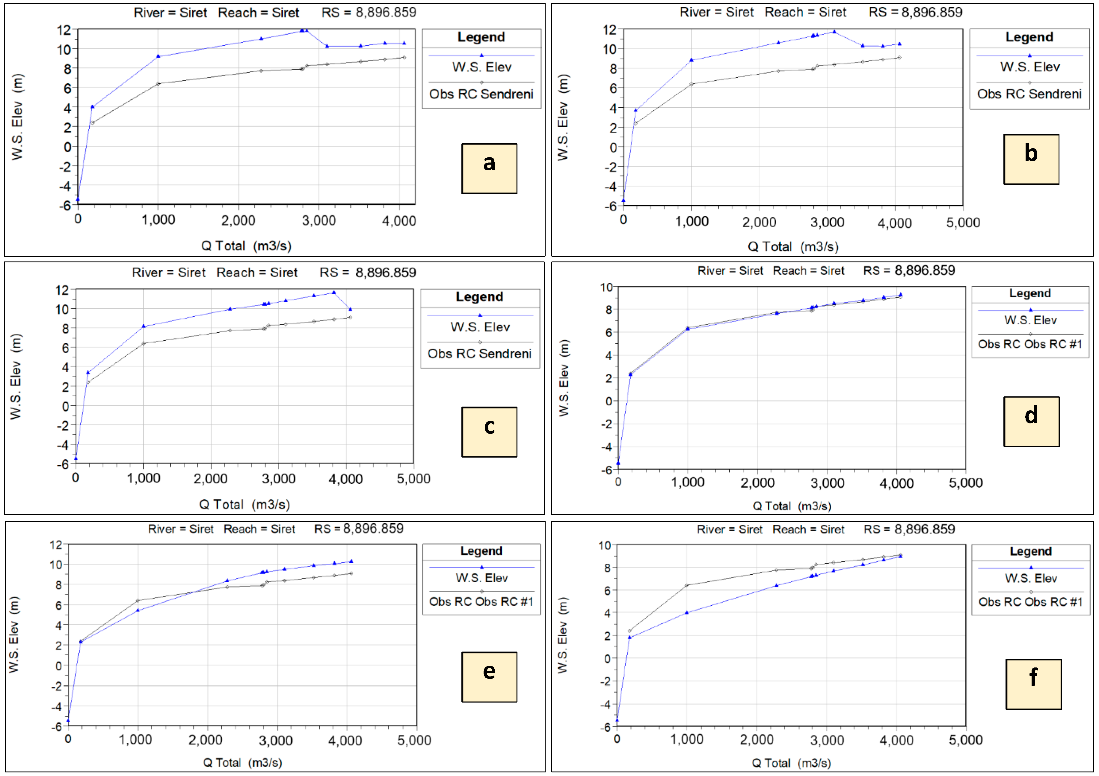
3.2. Numerical Simulation

In order to assess the flood extent, the event was simulated in the HEC-RAS software. The flood maps developed for this research paper were based on the 1D hydraulic model. In essence, the 1D model assumes that all the waters flow in the longitudinal direction [59]. To compute a 1D model for steady hydraulic simulation, the river floodplains need to be described by cross-sections. The equation for computing water flows in a one-dimensional model is composed of the conservation of mass and conservation of momentum equations between two nearby cross-sections [60,61]. The energy equation (Equation (1)) is as follows [62]:
Y 1 + Z 1 + a 1 V 1 2 2 g + h e   = Y 2 + Z 2 + a 2 V 2 2 2 g
where Y1 and Y2 represent water depths at the cross-section, Z1 and Z2 are the elevations of the main channel inverts, V1 and V2 are the average velocities, α1 and α2 describe the coefficients of mass momentum speed, g is the gravitational acceleration, and he is the energy head loss.
Romanian legislation enforces the application of the “Methodological Regulation about How to Prepare and What Is the Content of Flood Risk Maps”, which is in accordance with the Directive 2007/60/EC and the Guide for Reporting under the Floods Directive [63]. These classify the flood risk probability into three classes. Based on water depth from a flood event extent, the flood risk classes are as follows:
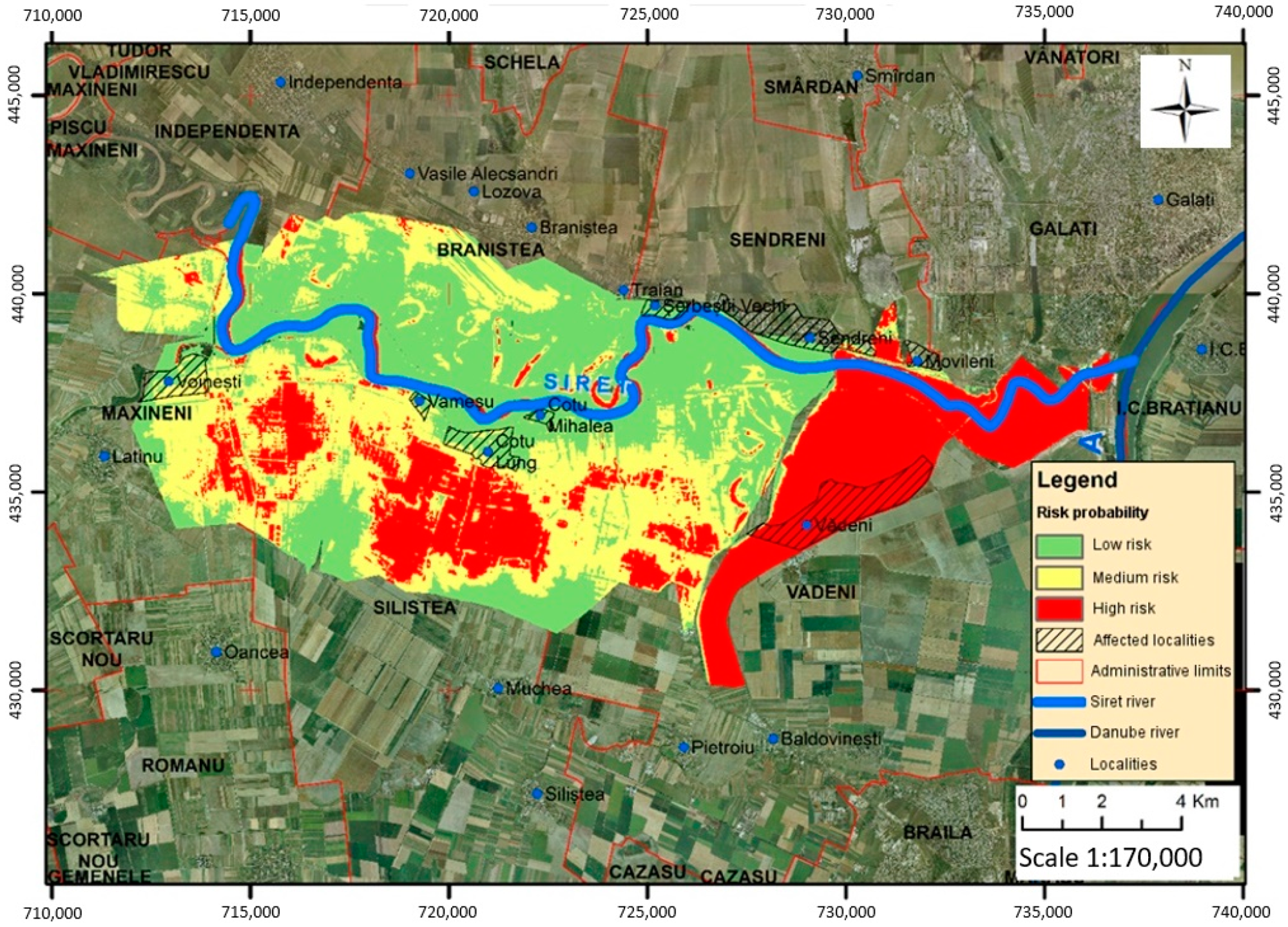
  • Depth < 0.5 m—low flood risk: in this case, the flood extent does not present any hazard to the people and has a low impact on the economic and sociocultural life. Moreover, this category of flood risk presents little difficulty in evacuation of habitants.
  • 0.5 m < Depth < 1.5 m—medium flood risk: in this case, the flood hazard may affect a region to a greater extent. There may be some difficulties in case of people evacuation, and there may be a medium to high influence on the economic and sociocultural indicators.
  • Depth > 1.5 m—high flood risk: this class represents an unwelcome situation where the flood hazard has a very high impact on the people, economy, infrastructure, and environmental and cultural indicators.
Thus, the development of flood risk and hazard maps needs to show some important elements of flood scenarios, such as the flood extent, the water surface elevation, water depth, water velocities, and discharge at different critical cross-sections. To achieve the main purpose of this paper, it is necessary to follow some important steps. Figure 10 presents the steps of collecting, preprocessing, and postprocessing of data that are necessary in order to develop the flood and hazard maps in the case of various flood scenarios.

4. Results and Discussion

The proposed area for this research paper is the part of the lower Siret River that was most affected during the 2010 flood event. The terrain model of the selected area was created by combining the LiDAR DEM and the bathymetric depth sounding data using the ArcGIS Topo-to-Raster interpolator and by resampling the raster to obtain a 0.5 × 0.5 m/pixel DEM (Figure 11).
Topography data to compute the schematic type for the HEC-RAS one-dimensional model was composed of a set of 88 digitized cross-sections. The maximum distance between the cross-sections was 75 m, and the minimum distance was 25 m. These distances depend on the sinuousness of the river. Where the river course is straighter, the distance between the cross-sections may be increased; conversely, where the river course is very meandering, additional cross-sections are necessary in order to describe the geometry of the main river channel (Figure 12) more accurately. Cross-sections cover at least the width of the river and the possible flooding area.
The calibration of the channel flow was obtained by modifying the Manning’s coefficient values according to Chow [64] in order to obtain the rating curve profile presented in Figure 13, with incertitude of ±10 cm. By applying a Manning’s coefficient between 0.07 and 0.02, the 0.04 value was chosen as the best value. The choice of 0.04 as the default value is in accordance with the channel composition, which is clean and winding, with some pools and shoals [37,65,66]. As shown in Figure 14, the correlation between the WSE values of the rating curve corresponding to the 2010 flood event and the modeled WSE elevation values prove the best fit for the Manning value of 0.04.
Major riverbed roughness values represent one of the important aspects of any hydraulic model. They help to define the floodplain extent and flow velocity out of the main river channel correctly. In fact, it is almost impossible to determine the roughness by in situ measurements, so roughness is usually estimated from alternative sources, such as pedological maps, orthophotomaps or LANDSAT satellite imagery [67,68,69]. Based on the physical characteristics of the major riverbed, seven types of roughness values were used (see Table 1).
Based on the available orthophotomap (Figure 15), a classified map with seven different roughness classes, presented in Table 1, was generated. The result of the digitized polygons for each roughness coefficient is highlighted by a color ramp and represented in Figure 16. In order to input the roughness values for the major riverbed automatically to HEC, the roughness coefficient distribution is converted to raster format (Figure 17).
The water surface elevation from the river gauge station was converted to terrain reference elevation using Equation (2):
W S E B S C = W S E G S + Z 0 G S
where WSEBSC represents the water surface elevation for the altimetric Black Sea 1975 Constanta Height Datum, WSEGS represents the water surface elevation given at the gauge station, Z0−GS is equal to 239 cm and represents the elevation of the zero-gauge station value above the Black Sea 1975 Constanta Height Datum.
In order to develop the flood extent for the 2010 event by applying Equation (2), the following water surface elevations for the mentioned return periods (N%) were calculated:
  • N10%—flow discharge Q = 2280 m3 s−1; WSEBSC = 773 cm;
  • N5%—flow discharge Q = 2850 m3 s−1, WSEBSC = 820 cm;
  • N2%—flow discharge Q = 3520 m3 s−1, WSEBSC = 867 cm;
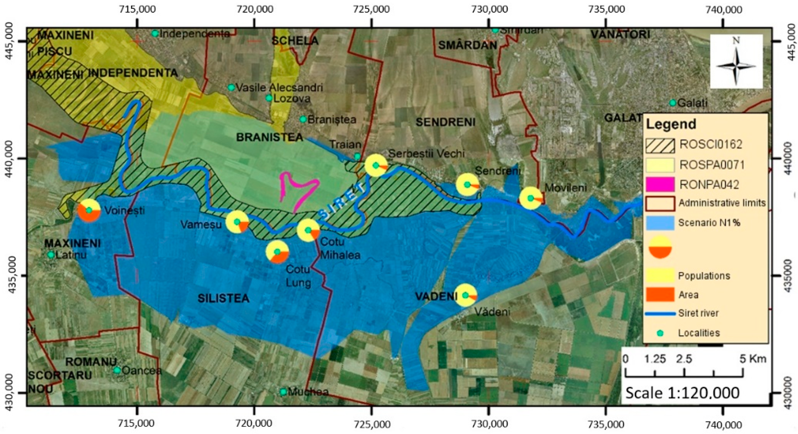
  • N1%—flow discharge Q = 4060 m3 s−1, WSEBSC = 906 cm.
Following the calibration of the entire geometric model in HEC-RAS, eight different discharge rate scenarios were modeled, from 500 to 4060 m3 s−1 flow discharge, in order to assess the evolution and gradual expansion of the flood extent. The water surface elevation results for the four important scenarios of N10% (10-year flood event), N5% (20-year flood event), N2% (50-year flood event) and N1% (100-year flood event) are presented in Figure 18.
When analyzing the four representative cross-section (Figure 18) profiles, it can be observed that the WSE elevation varies from the 12.2 to 13.5 m in the upstream cross-section (RS = 32,187.63, Figure 18) and from 6.3 to 8.2 m in the downstream cross-section (RS = 875.99, Figure 18). At the confluence with the Danube River, the WSE of the Siret River decreases rapidly due to the fact that elevations in the downstream part are lower those upstream. The slope of the energy grade losses is 0.015%.
In order to develop the flood extent maps for the studied area, a steady flow analysis was performed for each of the eight scenarios of flow discharge. The input boundary condition is presented in Table 2. Scenarios 1, 2, 3, and 5 were additionally computed to assess the other cases of flood extent and to compare the flooded to the nonflooded area. Each model gives different results of the flood extent.
The floodplain extent maps were developed using all the input data (elevations, gauge station values, Manning’s coefficients, river geometric scheme, levees, bank points, bridge geometric schemes). All the results, especially the main ones for this study (the WSE and velocity distribution map, as shown in Figure A3, and the depth range map and river power map, as shown in Figure A4) were extracted from HEC-RAS through HEC-GeoRAS and were incorporated in GIS software. Moreover, a statistical comparison was performed to assess the correlation between water velocity and water surface elevation data (Figure A5), and the correlation between water velocity and river power distribution (Figure A6). The delineated water surface extents, which represent the flooded area for the four return periods and four supplementary scenarios, are presented in Figure 19 and Figure 20.
Due to the fact that the digital terrain model covers only a part of the studied major riverbed, some of the localities that are in the major riverbed were not included in the modeling. However, they also have a low to medium flood risk (Figure 21).
According to correctly, the presented modeled scenario—N1% from Figure 22—represents a medium risk probability, while 0.1% represents high risk. Depending on the depths resulting from the modeling, the depth-specific pixels were reclassified into three classes: class 1, less than 0.5 m, is represents low risk; class 2, ranging from 0.5 to 1 m, represents medium risk; and class 3, greater than 1.5 m, represents high risk. Figure 22 represents the rasterized image of risk classes of localities which may be subject to an N1% medium risk.
The consequences of floods on the environment make up another series of key indicators. Several types of protected areas (Figure 23) have been identified: one special bird protection area (ROSPA0071) with the two bodies, Pădurea Neagră (the Black Forest) and Pădurea Dumbrăvița (Dumbrăviţa Forest); one site of community importance (ROSCI0162); and one reservation of interest (RONPA042), Balta Potcoava (Potcoava Swamp). All three protected areas are located in the floodplain of the Lower Siret (study area) and cover a total area of about 4725 ha.

5. Conclusions

The present study shows that flood extent maps at different discharge scenarios and return periods may be obtained when applying innovative in situ methods and materials. In this regard, the simulation of different flood scenarios helps to attain important information about the areas likely to be flooded. By analyzing Figure 19a, it is observed that a 500 m3 s−1 flow discharge represents a small value that does not generate a flood extent. In this case, the total water-covered area is 393 ha. By increasing the discharge rate to 1000 m3 s−1 in the middle part of the analyzed river section, the flow extends up to left and right levees. This happens especially in those sections where the course of the river is very meandering, as indicated by the red tags in Figure 19b. In this case, the flooded area increases by 61.5 ha as compared to the first scenario. The yellow and green tags (Figure 19c,d) for the 1500 and 2280 m3 s−1 (10-year return period scenario) scenarios show that the water surface elevations exceed the main channel limits in almost all cases, but only in the places where the sinuosity of the river is accentuated. The discharge rate equal to a 10-year return period (Q = 2280 m3 s−1) represents an 861 ha water-covered area, which is twice as much as the result from the first scenario. In the case of Q = 500 m3 s−1, the maximum value of water depth is 12 m; whereas, in the case of a 10-year return period, the maximum water depth values increase by 5 m.
For Q = 2850 m3 s−1 (N5%) and Q = 3520 m3 s−1 (N2%), the water levels are 8.20 and 8.67 m, respectively. In these cases, the water exceeds the right and left banks up to right and left levees, for the entire minor river channel (Figure 20a–d). The water depth level for the 100-year return period increases above that of the 50-year return period by 0.39 m. The total water-covered area for the last flood scenario is 15,500 ha. The flood extent includes the entire study area, with the limits imposed by the geometric scheme of the floodplain. The water depth increases by more than 1 m when compared to the previous scenarios. The maximum depth recorded is 19.5 m, in the downstream of the study area.
According to Directive 2007/60/EC, the consequences that floods have on infrastructure represent an important aspect affecting the economies of the EU Member States. Following the distance evaluation for each category of roads, 6 km of European roads, 9 km of national roads, 2 km of the county roads, and 2.5 km of communal roads can be considered as subject to the medium flood risk.
The bathymetric measurements represent the most important phase when achieving the main purpose of the flood risk and hazard map development process. The method used for bathymetric measurement and land surveying is applicable to different types of river courses. The DTM for major and minor riverbeds of the lower course (Danube–Șendreni–Independența), obtained by combining the LiDAR or UAV airborne techniques with the ground bathymetry and topography techniques, represents a unique and new DTM for this area, which generates a result with a correlation factor of R2 = 0.98. This element contributes 90% to obtaining correct results from hydraulic modeling and simulations. In order to achieve a precise digital elevation model, the precision of topographic and bathymetric measurements should be ±1–10 cm horizontally and ±5–15 cm vertically.
A critical parameter in accurately defining geometric elements for hydraulic modeling in HEC-RAS is the resulting digital elevation model. The key of a geometric model for the hydraulic simulation is influenced by the cross-sections, which are arranged at a width of about 2 × 1 river width (B), if the course of the river is sinuous. The lower course of the Siret River, i.e., the chosen study area, is a combined course, where there are linear areas; thus, the distance between the digitized cross-sections can reach up to 2 × 10 river widths (B). Cross-sections require a denser arrangement when there are declivity decreases or roughness coefficient alterations of the ground in the minor riverbed.
The results of hydraulic modeling in the HEC-RAS program are directly influenced by the coefficient of roughness (Manning’s roughness coefficient). The minor riverbed of the lower course of the Siret River is entirely characterized by a sandy-clay soil with multiple meanders and sandbanks. All of them are formed by sediment migration; stones are rare and appear only in the areas where rehabilitation or bank improvement works have been conducted. Therefore, it is appropriate to use a roughness coefficient of 0.040. The major riverbed has different land categories; consequently, the roughness coefficients vary from one category to another, ranging from 0.012 to 0.10. The roughness coefficient is the critical parameter for calibrating the HEC-RAS model. It has to be adjusted in such way that the differences between the modeled flow-rating curve and the measured flow-rating curve at the hydrographic stage should not exceed ±10–15 cm.
A new approach in this research paper is the automatic assignment of roughness coefficients depending on the boundaries of the polygons that characterize each category of land and are digitized at the stage of geometric modeling using the GIS programs.
Once the calibration of the HEC-RAS model was completed, the hazard and flood risk maps were generated for the study area, i.e., the lower course of the Siret River. After analyzing the obtained correlations between the flow rate and the river power, it may be mentioned that the river power is directly influenced by the water flow rate. This statement is supported by the results obtained when correlating the indicator R2 = 0.7166 with the maximum flow of 4060 m3 s−1. In fact, this is the reason why sudden changes in the watercourse might occur over time in some areas, especially where the sinuousness of the river is more pronounced.
The risk and hazard maps have been compiled in accordance with the Floods Directive 2007/60/EC, except for the scenario with an overflow probability of N0.1%, for which there are no historical records. Overall, there are over 9500 inhabitants, 19.5 km of road infrastructure, 16.5 km of the railway infrastructure, eight social patrimony elements, and three environmental indicators which are vulnerable and exposed to a medium risk of producing a hazard once every 100 years.
The novelty of this research is based on the concept that shows how to use multiple combined techniques and methods to assess flood extent and to subsequently use this information for further purposes (e.g., flood defense strategies, flood management strategies, investment promotion activities, infrastructure damage prevention).
Last but not least, ideas of a future plan have emerged from the analysis of the obtained results, implying the use of coupled 1D/2D simulation models. It is known that 2D simulations require much more complex input data and that collaboration agreements are needed in order to establish and build modern research projects on environmental issues. Bathymetric equipment, high-accuracy topography data, and cutting-edge software programs are necessary to enable such research. The comparison of modeling results could also take place among 1D, 2D, or coupled 1D/2D models.

Author Contributions

M.A. and A.R. performed the measurements, established the methodology, and validated and analyzed the data; M.C. and V.A.C. conducted formal analysis; L.P.G. and C.I. supervised the progress of the teamwork; M.A. conducted the statistical analysis and prepared the manuscript. All authors have read and agreed to the published version of the manuscript.

Funding

This work was supported by the project “EXPERT”, financed by the Romanian Ministry of Research and Innovation, Contract No. 14PFE/17.10.2018.

Acknowledgments

This work was supported by the project “Excellence, performance and competitiveness in the Research, Development and Innovation activities at “Dunarea de Jos” University of Galati”, acronym “EXPERT”. This work was financed by the Romanian Ministry of Research and Innovation in the framework of Program 1—Development of the national research and development system, Sub-program 1.2—Institutional Performance—Projects for financing excellence in Research, Development and Innovation, Contract No. 14PFE/17.10.2018. The linguistic review of the present article was made by Antoanela Marta Mardar, member of the Research Center “Interface Research of the Original and Translated Text. Cognitive and Communicative Dimensions of the Message”, Faculty of Letters, “Dunărea de Jos” University of Galați, Romania.

Conflicts of Interest

The authors declared no conflict of interest.

Appendix A

Figure A1. Bathymetric cross-section profiles (blue dots) and bank points (yellow dots), measured from downstream to upstream, for the S1–S4 sections of the 35 km section of the Siret River.
Sustainability 12 06588 g0a1
Figure A2. Bathymetric cross-section profiles (blue dots) and bank points (yellow dots), measured from downstream to upstream, for the S5–S9 sections of the 35 km section of the Siret River.
Sustainability 12 06588 g0a2
Figure A3. Water velocity distribution: (a) Q = 2820 m3 s−1, (b) Q = 2850 m3 s−1, (c) Q = 3520 m3 s−1, and (d) Q = 4060 m3 s−1.
Sustainability 12 06588 g0a3
Figure A4. River power distribution: (a) Q = 2820 m3 s−1, (b) Q = 2850 m3 s−1, (c) Q = 3520 m3 s−1, and (d) Q = 4060 m3 s−1.
Sustainability 12 06588 g0a4
Figure A5. Three-dimensional matrix correlation between river distance, water velocity flow, and water surface elevation: (a) N10%, (b) N5%, (c) N2%, and (d) N1%.
Sustainability 12 06588 g0a5
Figure A6. Pearson correlation graph between river water velocity flow and river power results: (a) N10% (Q = 2820 m3 s−1), (b) N5% (Q = 2850 m3 s−1), (c) N2% (Q = 3520 m3 s−1), and (d) N1% (Q = 4060 m3 s−1).
Sustainability 12 06588 g0a6

References

  1. Quirogaa, V.M.; Kurea, S.; Udoa, K.; Manoa, A. Application of 2D numerical simulation for the analysis of the February 2014 Bolivian Amazonia flood: Application of the new HEC-RAS version 5. Ribagua 2016, 3, 25–33. [Google Scholar] [CrossRef] [Green Version]
  2. Luu, C.; Tran, H.X.; Pham, B.T.; Al-Ansari, N.; Tran, T.Q.; Duong, N.Q.; Dao, N.H.; Nguyen, L.P.; Nguyen, D.H.; Ta, H.T.T.; et al. Framework of Spatial Flood Risk Assessment for a Case Study in Quang Binh Province, Vietnam. Sustainability 2020, 12, 3058. [Google Scholar] [CrossRef] [Green Version]
  3. Mysiak, J.; Testella, F.; Bonaiuto, M.; Carrus, G.; De Dominicis, S.; Cancellieri, U.G.; Firus, K.; Grifoni, P. Flood risk management in Italy: Challenges and opportunities for the implementation of the EU Floods Directive (2007/60/EC). Nat. Hazards Earth Syst. Sci. 2013, 13, 2883–2890. [Google Scholar] [CrossRef]
  4. European Environment Agency. Directive 2007/60/EC of the European Parliament and of the Council on the Assessment and Management of Flood Risks. Available online: https://www.eea.europa.eu/policy-documents/directive-2007-60-ec-of (accessed on 20 April 2020).
  5. Spachinger, K.; Dorner, W.; Metzka, R.; Serrhini, K.; Fuchs, S. Flood Risk and Flood Hazard Maps–Visualisation of Hydrological Risks. IOP Conf. Ser. Earth Environ. Sci. 2008, 4, 012043. [Google Scholar] [CrossRef] [Green Version]
  6. Lo, S.W.; Wu, J.H.; Lin, F.P.; Hsu, C.H. Visual sensing for urban flood monitoring. Sensors 2015, 15, 20006–20029. [Google Scholar] [CrossRef] [PubMed] [Green Version]
  7. Murphy, A.T.; Gouldby, B.; Cole, S.J.; Moore, R.J.; Kendall, H. Real-time flood inundation forecasting and mapping for key railway infrastructure: A UK case study. E3S Web Conf. 2016, 7, 18020. [Google Scholar] [CrossRef] [Green Version]
  8. Van Leeuwen, B.; Tobak, Z.; Kovács, F. Sentinel-1 and -2 Based near Real Time Inland Excess Water Mapping for Optimized Water Management. Sustainability 2020, 12, 2854. [Google Scholar] [CrossRef] [Green Version]
  9. Domeneghetti, A.; Schumann, G.J.-P.; Tarpanelli, A. Preface: Remote Sensing for Flood Mapping and Monitoring of Flood Dynamics. Remote Sens. 2019, 11, 943. [Google Scholar] [CrossRef] [Green Version]
  10. Arseni, M.; Roșu, A.; Bocăneală, C.; Constantin, D.-E.; Georgescu, P.L. Flood hazard monitoring using GIS and remote sensing observations. Carpathian J. Earth Environ. Sci. 2017, 12, 329–334. [Google Scholar]
  11. Abu-Abdullah, M.M.; Youssef, A.M.; Maerz, N.H.; Abu-Alfadail, E.; Al-Harbi, H.M.; Al-Saadi, N.S. A flood riskmanagement programofwadi bayshdam on the downstream area: An integration of hydrologic and hydraulicmodels, Jizan region, KSA. Sustainability 2020, 12, 1069. [Google Scholar] [CrossRef] [Green Version]
  12. Ruiz-Bellet, J.L.; Balasch, J.C.; Tuset, J.; Barriendos, M.; Mazon, J.; Pino, D. Historical, hydraulic, hydrological and meteorological reconstruction of 1874 Santa Tecla flash floods in Catalonia (NE Iberian Peninsula). J. Hydrol. 2015, 524, 279–295. [Google Scholar] [CrossRef] [Green Version]
  13. Atallah, M.; Hazzab, A.; Seddini, A.; Ghenaim, A.; Korichi, K. Inundation maps for extreme flood events: Case study of Sidi Bel Abbes city, Algeria. J. Water Land Dev. 2018, 37, 19–27. [Google Scholar] [CrossRef]
  14. Rai, P.K.; Dhanya, C.T.; Chahar, B.R. Coupling of 1D models (SWAT and SWMM) with 2D model (iRIC) for mapping inundation in Brahmani and Baitarani river delta. Nat. Hazards 2018, 92, 1821–1840. [Google Scholar] [CrossRef]
  15. David, A.; Schmalz, B. Flood hazard analysis in small catchments: Comparison of hydrological and hydrodynamic approaches by the use of direct rainfall. J. Flood Risk Manag. 2020. [Google Scholar] [CrossRef]
  16. Bures, L.; Roub, R.; Sychova, P.; Gdulova, K.; Doubalova, J. Comparison of bathymetric data sources used in hydraulic modelling of floods. J. Flood Risk Manag. 2019, 12. [Google Scholar] [CrossRef] [Green Version]
  17. Liu, Z.; Merwade, V.; Jafarzadegan, K. Investigating the role of model structure and surface roughness in generating flood inundation extents using one- and two-dimensional hydraulic models. J. Flood Risk Manag. 2019, 12. [Google Scholar] [CrossRef] [Green Version]
  18. Jalil, S.; Qasim, J.M.; Jalil, S.A. Numerical Modelling of Flow over Single-Step Broad-Crested Weir Using FLOW-3D and HEC-RAS. Polytechnic 2016, 6, 435–448. [Google Scholar]
  19. Salazar, A.; Vargas, J.; Rivera, L.; Robledo, V.; Chang, P.; Temgoua, A.G.T. Comparative study of the HEC-RAS, IBER and Flow 3D Softwares in studying flow characteristics across a dynamic meander in Colombia. In Proceedings of the Canadian Society for Civil Engineering Annual Conference, Montreal, QC, Canada, 12–15 June 2019. [Google Scholar]
  20. Patel, A.; Katiyar, S.K.; Prasad, V. Performances evaluation of different open source DEM using Differential Global Positioning System (DGPS). Egypt J. Remote Sens. Space Sci. 2016, 19, 7–16. [Google Scholar] [CrossRef] [Green Version]
  21. Anees, M.T.; Abdullah, K.; Nawawi, M.N.M.; Ab Rahman, N.N.N.; Piah, A.R.M.; Zakaria, N.A.; Syakir, M.; Omar, A.M. Numerical modeling techniques for flood analysis. J. Afr. Earth Sci. 2016, 124, 478–486. [Google Scholar] [CrossRef]
  22. Vozinaki, A.E.K.; Morianou, G.G.; Alexakis, D.D.; Tsanis, I.K. Comparing 1D and combined 1D/2D hydraulic simulations using high-resolution topographic data: A case study of the Koiliaris basin, Greece. Hydrol. Sci. J. 2017, 62, 642–656. [Google Scholar] [CrossRef]
  23. Arseni, M.; Rosu, A.; Georgescu, L.P.; Iticescu, I.; Calmuc, V.; Calmuc, C. Impact of expansion and contraction coefficients on water surface profiles. New Technol. Prod. Mach. Manuf. Technol. 2019, 26, 60–65. [Google Scholar]
  24. Ahmad, H.F.; Alam, A.; Sultan, M.; Professor, B.; Ahmad, S. One Dimensional Steady Flow Analysis Using HEC-RAS-A case of River Jhelum, Jammu and Kashmir. Eur. Sci. J. 2016, 12, 1857–7881. [Google Scholar] [CrossRef]
  25. Agrawal, R. Flood Analysis Of Dhudhana River In Upper Godavari Basin Using HEC-RAS. Int. J. Eng. Res. 2016, 1, 188–191. [Google Scholar] [CrossRef]
  26. Grimaldi, S.; Li, Y.; Walker, J.P.; Pauwels, V.R.N. Effective Representation of River Geometry in Hydraulic Flood Forecast Models. Water Resour. Res. 2018, 54, 1031–1057. [Google Scholar] [CrossRef]
  27. Iticescu, C.; Georgescu, L.P.; Murariu, G.; Topa, C.; Timofti, M.; Pintilie, V.; Arseni, M. Lower danube water quality quantified through WQI and multivariate analysis. Water 2019, 11, 1305. [Google Scholar] [CrossRef] [Green Version]
  28. Rojas, O.; Mardones, M.; Rojas, C.; Martínez, C.; Flores, L. Urban growth and flood disasters in the coastal river basin of South-Central Chile (1943–2011). Sustainability 2017, 9, 195. [Google Scholar] [CrossRef] [Green Version]
  29. Adeva-Bustos, A.; Alfredsen, K.; Fjeldstad, H.P.; Ottosson, K. Ecohydraulic modelling to support Fish Habitat Restoration Measures. Sustainability 2019, 11, 1500. [Google Scholar] [CrossRef] [Green Version]
  30. Ardıçlıoğlu, M.; Kuriqi, A. Calibration of channel roughness in intermittent rivers using HEC-RAS model: Case of Sarimsakli creek, Turkey. SN Appl. Sci. 2019, 1, 1–9. [Google Scholar] [CrossRef] [Green Version]
  31. Habib-ur-Rehman; Chaudhry, M.A.; Naeem, U.A.; Hashmi, H.N. Performance evaluation of 1-D numerical model HEC-RAS towards modeling sediment depositions and sediment flushing operations for the reservoirs. Environ. Monit. Assess. 2018, 190, 433. [Google Scholar] [CrossRef]
  32. Ben Khalfallah, C.; Saidi, S. Spatiotemporal floodplain mapping and prediction using HEC-RAS-GIS tools: Case of the Mejerda river, Tunisia. J. Afr. Earth Sci. 2018, 142, 44–51. [Google Scholar] [CrossRef]
  33. Huţanu, E.; Mihu-Pintilie, A.; Urzica, A.; Paveluc, L.E.; Stoleriu, C.C.; Grozavu, A. Using 1D HEC-RAS Modeling and LiDAR Data to Improve Flood Hazard Maps Accuracy: A Case Study from Jijia Floodplain (NE Romania). Water 2020, 12, 1624. [Google Scholar] [CrossRef]
  34. Dasallas, L.; Kim, Y.; An, H. Case Study of HEC-RAS 1D–2D Coupling Simulation: 2002 Baeksan Flood Event in Korea. Water 2019, 11, 2048. [Google Scholar] [CrossRef] [Green Version]
  35. Dimitriadis, P.; Tegos, A.; Oikonomou, A.; Pagana, V.; Koukouvinos, A.; Mamassis, N.; Koutsoyiannis, D.; Efstratiadis, A. Comparative evaluation of 1D and quasi-2D hydraulic models based on benchmark and real-world applications for uncertainty assessment in flood mapping. J. Hydrol. 2016, 534, 478–492. [Google Scholar] [CrossRef]
  36. Amarnath, C.R.; Thatikonda, S. Study on Backwater Effect Due to Polavaram Dam Project under Different Return Periods. Water 2020, 12, 576. [Google Scholar] [CrossRef] [Green Version]
  37. Arseni, M.; Voiculescu, M.; Georgescu, L.P.; Iticescu, C.; Rosu, A. Testing Different Interpolation Methods Based on Single Beam Echosounder River Surveying. Case Study: Siret River. ISPRS Int. J. Geoinf. 2019, 8, 507. [Google Scholar] [CrossRef] [Green Version]
  38. Nacu, V.; Stoian, I.; Vele, D.; Arseni, M. Geodetic Methods Regarding the Crustal Movements and Earthquake Prediction. In Modern Technologies for the 3rd Millennium; Nistor, S., Popoviciu, G.A., Eds.; Medimond: Bologna, Italy, 2016; pp. 27–33. [Google Scholar]
  39. National Administration Attributions. Romanian Waters. Available online: http://www.rowater.ro/EPRI%20%20Harti%20cu%20zone%20risc%20la%20inundatii/APSFR_Siret.jpg (accessed on 20 April 2020).
  40. Romanescu, G. Floods in the Siret and Pruth Basins; Springer: Berlin/Heidelberg, Germany, 2013; pp. 99–120. [Google Scholar] [CrossRef]
  41. Romanescu, G.; Stoleriu, C. Causes and effects of the catastrophic flooding on the Siret River (Romania) in July–August 2008. Nat. Hazards 2013, 69, 1351–1367. [Google Scholar] [CrossRef]
  42. Clearing House Mechanism Romania. Available online: http://biodiversitate.mmediu.ro/rio/natura2000/static/pdf/rosci0162.pdf (accessed on 20 April 2020).
  43. Murariu, G.; Puscasu, G.; Gogoncea, V.; Angelopoulos, A.; Fildisis, T. Non-Linear Flood Assessment with Neural Network. AIP Conf. Proc. 2010, 1203, 812–819. [Google Scholar] [CrossRef]
  44. SOUTH S82V Technical Specifications. Available online: https://geo-matching.com/gnss-receivers/s82v (accessed on 19 July 2019).
  45. Djaja, K.; Putera, R.; Rohman, A.F.; Sondang, I.; Nanditho, G.; Suyanti, E. The Integration of Geography Information System (Gis) and Global Navigation Satelite System-real Time Kinematic (Gnss-rtk) for Land Use Monitoring. Int. J. GEOMATE 2017, 13, 2186–2990. [Google Scholar] [CrossRef]
  46. Wang, C.; Higgins, M. Assessment of Commercial Network RTK User Positioning Performance over Long Inter-Station Distances. J. Glob. Position. Syst. 2010. [Google Scholar] [CrossRef]
  47. Parr, A.D.; Milburn, S.; Malone, T.; Bender, T. A Model Study of Bridge Hydraulics, 2nd ed.; Kansas Department of Transportation, Bureau of Materials & Research: Topeka, KS, USA, 2010. [Google Scholar]
  48. Lee, K.T.; Ho, Y.H.; Chyan, Y.J. Bridge blockage and overbank flow simulations using HEC-RAS in the Keelung River during the 2001 Nari Typhoon. J. Hydraul. Eng. 2006, 132, 319–323. [Google Scholar] [CrossRef]
  49. Hunt, J.; Brunner, G.W.; Larock, B.E. Flow Transitions in Bridge Backwater Analysis. J. Hydraul. Eng. 1999, 125, 981–983. [Google Scholar] [CrossRef] [Green Version]
  50. Collings, S.; Botha, E.; Anstee, J.; Campbell, N. Depth from Satellite Images: Depth Retrieval Using a Stereo and Radiative Transfer-Based Hybrid Method. Remote Sens. 2018, 10, 1247. [Google Scholar] [CrossRef] [Green Version]
  51. Zhao, J.; Zhao, X.; Zhang, H.; Zhou, F. Improved Model for Depth Bias Correction in Airborne LiDAR Bathymetry Systems. Remote Sens. 2017, 9, 710. [Google Scholar] [CrossRef] [Green Version]
  52. Mandlburger, G.; Hauer, C.; Wieser, M.; Pfeifer, N. Topo-Bathymetric LiDAR for Monitoring River Morphodynamics and Instream Habitats—A Case Study at the Pielach River. Remote Sens. 2015, 7, 6160–6195. [Google Scholar] [CrossRef] [Green Version]
  53. Pan, Z.; Glennie, C.; Hartzell, P.; Fernandez-Diaz, J.; Legleiter, C.; Overstreet, B. Performance Assessment of High Resolution Airborne Full Waveform LiDAR for Shallow River Bathymetry. Remote Sens. 2015, 7, 5133–5159. [Google Scholar] [CrossRef] [Green Version]
  54. Zhao, J.; Zhao, X.; Zhang, H.; Zhou, F. Shallow Water Measurements Using a Single Green Laser Corrected by Building a Near Water Surface Penetration Model. Remote Sens. 2017, 9, 426. [Google Scholar] [CrossRef] [Green Version]
  55. Quadros, N.; Collier, P. Integration of bathymetric and topographic LiDAR: A preliminary investigation. Int. Arch. Photogramm. Remote Sens. Spat. Inf. Sci. 2008, 36, 1299–1304. [Google Scholar]
  56. Saylam, K.; Hupp, J.R.; Averett, A.R.; Gutelius, W.F.; Gelhar, B.W. Airborne lidar bathymetry: Assessing quality assurance and quality control methods with Leica Chiroptera examples. Int. J. Remote Sens. 2018, 39, 2518–2542. [Google Scholar] [CrossRef]
  57. Kinzel, P.J.; Legleiter, C.J.; Nelson, J.M. Mapping River Bathymetry with a Small Footprint Green LiDAR: Applications and Challenges. J. Am. Water Resour. Assoc. 2013, 49, 183–204. [Google Scholar] [CrossRef]
  58. International Hydrographic Organization. Standards for Hydrographic Surveys, Special Publication No. 44, 5th ed.; International Hydrographic Bureau: Monaco, Monaco, 2008. [Google Scholar]
  59. Cook, A.C. Comparison of One-Dimensional HEC-RAS with Two-Dimensional FESWMS Model in Flood Inundation Mapping; Purdue University: West Lafayette, IN, USA, 2008. [Google Scholar]
  60. Shahiriparsa, A.; Heydari, M.; Sadeghian, M.S.; Moharrampour, M. Flood Zoning Simulation by HEC-RAS Model (Case Study: Johor River-Kota Tinggi Region). J. River Eng. 2013, 1. [Google Scholar] [CrossRef]
  61. Wang, C.H. Application of HEC-RAS Model in Simulation of Water Surface Profile of River. Appl. Mech. Mater. 2014, 641, 232–235. [Google Scholar] [CrossRef]
  62. US Army Corps of Engineers Institute for Water Resources Hydrologic Engineering Center. HEC-RAS River Analysis System Hydraulic Reference Manual Version 5.0, 2016. Available online: https://www.hec.usace.army.mil/software/hec-ras/documentation/HEC-RAS%205.0%20Reference%20Manual.pdf (accessed on 25 April 2020).
  63. Chendeş, V.; Rădulescu, D.; Rândaşu, S.; Ion, B.; Achim, D.; Preda, A. Guidance for Reporting under the Floods Directive (Aspecte metodologice privind realizarea hartilor de risc la inundatii raportate in cadrul directivei 2007/60/EC). Hidrotechnica 2014, 59, 10–11. [Google Scholar]
  64. Chow, V.T. Open-Channel Hydraulics; McGraw-Hill: New York, NY, USA, 1959. [Google Scholar]
  65. Arseni, M.; Georgescu, P.L. Modern GIS Techniques for Determination of the Territorial Risks. Ph.D. Thesis, University “Dunarea de Jos”, Galati, Romania, 2018. [Google Scholar]
  66. Ichim, I.; Radoane, M. Channel sediment variability along a river: A case study of the Siret River (Romania). Earth Surf. Process. Landforms 1990, 15, 211–225. [Google Scholar] [CrossRef]
  67. Kumar Parhi, P.; Sankhua, R.N.; Roy, G.P. Calibration of Channel Roughness for Mahanadi River, (India) Using HEC-RAS Model. J. Water Resour. Prot. 2012, 4, 847–850. [Google Scholar] [CrossRef] [Green Version]
  68. Bricker, J.D.; Gibson, S.; Takagi, H.; Imamura, F. On the need for larger Manning’s roughness coefficients in depth-integrated tsunami inundation models. Coast. Eng. J. 2015, 57. [Google Scholar] [CrossRef]
  69. Mtamba, J.; van der Velde, R.; Ndomba, P.; Zoltán, V.; Mtalo, F. Use of Radarsat-2 and Landsat TM Images for Spatial Parameterization of Manning’s Roughness Coefficient in Hydraulic Modeling. Remote Sens. 2015, 7, 836–864. [Google Scholar] [CrossRef] [Green Version]
Figure 1. Maps of areas with a high level of anticipated flood risk: (a) location of the Siret Hydrographic Space; (b) the lower section of the Siret River, which is permanently affected by major floods [39].
Sustainability 12 06588 g001
Figure 2. Maximum historical flows recorded on Siret River and its tributaries [40,41].
Sustainability 12 06588 g002
Figure 3. The study area, located at the confluence of the Siret River with the Danube.
Sustainability 12 06588 g003
Figure 4. Rating curve values at the Sendreni gauge station during the 2010 flood year.
Sustainability 12 06588 g004
Figure 5. Cross-section profile of Galați-Brăila road bridge (km 0 + 0.780) measured on Siret River.
Sustainability 12 06588 g005
Figure 6. Cross-section profile of Liberty conveyor belt (km 1 + 0.03) measured on Siret River.
Sustainability 12 06588 g006
Figure 7. Cross-section profile of Barboși railway bridge (km 4 + 0.905) measured on Siret River.
Sustainability 12 06588 g007
Figure 8. Cross-section profile of Șendreni road bridge (km 8 + 0.860) measured on Siret River.
Sustainability 12 06588 g008
Figure 9. Instruments used for land, bathymetric, and photogrammetric surveying: (a,b) single-beam bathymetric equipment combined with GNSS receiver mounted on a fiberglass boat; (c) land surveying total station equipment used for bank measurement; (d) UAV equipment used for photogrammetric surveying in areas with difficult access; (e) GNSS receiver with RTK used for land surveying in bank areas.
Sustainability 12 06588 g009
Figure 10. The logical scheme regarding the execution phases of flood hazard and risk maps on a river.
Sustainability 12 06588 g010
Figure 11. Digital elevation model for the studied area composed of the combination of LiDAR DEM and bathymetric data collection points.
Sustainability 12 06588 g011
Figure 12. The ArcGIS geometric model for the studied river section obtained by using the HEC-GeoRAS tool.
Sustainability 12 06588 g012
Figure 13. Model calibration with HEC-RAS tool according to roughness: (a) n = 0.07, (b) n = 0.06, (c) n = 0.05, (d) n = 0.04, (e) n = 0.03, and (f) n = 0.02.
Sustainability 12 06588 g013
Figure 14. Statistical correlation between the rating curve elevation values and the modeled values, used for model calibration.
Sustainability 12 06588 g014
Figure 15. The 0.5 m accuracy orthophotomap used for land classification and for roughness coefficient assignment.
Sustainability 12 06588 g015
Figure 16. Roughness coefficient assignment using digitizing land polygons.
Sustainability 12 06588 g016
Figure 17. The rasterized map of roughness coefficient distributions.
Sustainability 12 06588 g017
Figure 18. The water surface elevation profiles for a 10-year flood event (blue profile line), 20-year flood event (magenta profile line), 50-year flood event (green profile line), and 100-year flood event (red profile line).
Sustainability 12 06588 g018
Figure 19. Flood extent simulated with HEC-RAS software: (a) Q = 500 m3 s−1, (b) Q = 1000 m3 s−1, (c) Q = 1500 m3 s−1, and (d) Q = 2280 m3 s−1.
Sustainability 12 06588 g019
Figure 20. Flood extent simulated with HEC-RAS software: (a) Q = 2500 m3 s−1, (b) Q = 2850 m3 s−1, (c) Q = 3520 m3 s−1, and (d) Q = 4060 m3 s−1.
Sustainability 12 06588 g020
Figure 21. The extent of flooded areas for the 10-year flood event (N10%), 20-year flood event (N5%), 50-year flood event (N2%), and 100-year flood event (N1%).
Sustainability 12 06588 g021
Figure 22. Flood risk map for the 1% scenario.
Sustainability 12 06588 g022
Figure 23. Protected flooded areas in case of the 100-year flood event—N1%.
Sustainability 12 06588 g023
Table 1. The n coefficients of roughness (Te Chow, 1959).
Category Description MinNormalMax
Major riverbed
Grassland0.0300.0350.050
Short grass0.0350.0400.045
Arable land0.0330.0450.055
Brushwood 0.0700.1100.160
Thick trees, knobs, broken branches0.0800.1200.140
Broadleaf trees, willows, thick leaves during the summer 0.1100.1500.200
Urban area
Asphalt, pavement 0.0120.0150.020
Table 2. The eight discharge (Q) scenarios for the development of flood extent maps (N%, the return period; Q m3 s−1, upstream discharge; n, main channel Manning coefficient; S%, downstream normal depth).
Scenarios12345678
Boundary
Qupstream5001000150022802500285035204060
Sdownstream0.0150.0150.0150.0150.0150.0150.0150.015
nmainchannel0.040.040.040.040.040.040.040.04
N%---N10%-N5%N2%N1%

