Article

Intelligent System for the Predictive Analysis of an Industrial Wastewater Treatment Process

1
Department of Electrical and Electronics Engineering, Universidad del Norte, Barranquilla 081007, Colombia
2
Department of Civil and Environmental Engineering, Universidad del Norte, Barranquilla 081007, Colombia
*
Author to whom correspondence should be addressed.
Sustainability 2020, 12(16), 6348; https://doi.org/10.3390/su12166348
Submission received: 4 July 2020 / Revised: 24 July 2020 / Accepted: 27 July 2020 / Published: 7 August 2020
(This article belongs to the Special Issue Sustainability in the Development of Water Systems Management)

Abstract

:
Considering the exponential growth of today’s industry and the wastewater results of its processes, it needs to have an optimal treatment system for such effluent waters to mitigate the environmental impact generated by its discharges and comply with the environmental regulatory standards that are progressively increasing their demand. This leads to the need to innovate in the control and management information systems of the systems responsible to treat these residual waters in search of improvement. This paper proposes the development of an intelligent system that uses the data from the process and makes a prediction of its behavior to provide support in decision making related to the operation of the wastewater treatment plant (WWTP). To carry out the development of this system, a multilayer perceptron neural network with 2 hidden layers and 22 neurons each is implemented, together with process variable analysis, time-series decomposition, correlation and autocorrelation techniques; it is possible to predict the chemical oxygen demand (COD) at the input of the bioreactor with a one-day window and a mean absolute percentage error (MAPE) of 10.8%, which places this work between the adequate ranges proposed in the literature.

1. Introduction

Pursuing the ideas outlined in the sustainable development goals (SDGs), countries have been showing concern for terrestrial ecosystems even more for the reuse and conservation of water quality. On this topic, one of the concerns that exists and will be resolved day by day is related to the contamination of liquid effluents that arise from industrial uses. According to standards established by the laws of most countries, industry must respond to certain requirements that allow for the reuse of the water products in its activity. Globally, the most common problem regarding the quality of effluent water in industries is eutrophication, the result of large amounts of nutrients (mainly phosphorus and nitrogen), which leads to the purity of the water being reduced [1]. Additionally, pH levels and the suspended solids index contribute significantly to water quality [2]. Thus, industry daily faces the challenge of treating wastewater as a result of its processes. The monitoring of this treatment yields a large volume of revealing data that can increase the efficiency in the removal of the contaminant load in the water. Faced with this problem, it is worth asking: Is it possible to create an intelligent system that can monitor the determining variables in the treatment of industrial wastewater? Can this intelligent system predict the parameters of water quality with a prudent margin of error? How could it check the operation of this system? This paper focuses on answering the previous questions.
Taking into account the exponential growth of industry at present and the amount of wastewater that its processes generate, it is essential for it to have an optimal treatment system for such effluents to mitigate the environmental impact generated by its discharges and comply with the environmental regulatory standards that increase their demand. This leads to innovation both in the treatment systems and in control and information management systems thereof to achieve a more efficient process, whose advantages have been evidenced in different developed countries [3]. The proposed approach is an intelligent system that uses the data from the biological stage of the process and makes a prediction of the behavior of bioreactors in a way that provides support in the decision making related to the operation of the wastewater treatment plant that can improve its operational efficiency. Implementing a continuous prediction of out-of-range values leads to taking timely preventive measures. As a result, water of a higher quality than required and bottleneck reduction because of the adaptation of microorganisms are some of the advantages obtained, which represent savings in operational costs.
A wastewater treatment plant (WWTP) is composed of different stages depending on the properties of the effluents to treat, but it most commonly takes advantage of either physical, chemical or biological treatments to take away pollutants [4]. The present work refers to industrial wastewater, which is that from the discharges of manufacturing industries [5], and uses data from the activated sludge process in the biological stage for developing an intelligent system, making use of machine learning algorithms that allow for automatic extraction of information from previous examples and infer about new data [6], achieving the forecasting of the chemical oxygen demand (COD), which is an indicator of water pollution and is a key variable to evaluate the efficiency of the WWTP process [7].

2. Related Works

Over the last decade, the amount and complexity of data have increased significantly thanks to the improvement in generation and storage of data, related to the cost reduction of them and the presence of more computational power [8]. Therefore, all this data now available can produce valuable information leading to better phenomenon comprehension, modeling and reproduction capable of providing some advantages and improvements to industrial processes [9]. Referring to water treatment plants, they integrated programmable logic controllers, supervisory control and data acquisition systems at the beginning of the XXI century [3]. Residential, agricultural, commercial and industrial effluents can be treated by WWTPs, each with its characteristics [10]. In the present research, mostly industrial effluent source studies are presented as the main topic of interest.
The analysis of the process of a WWTP can be classified as a complex control problem, which behaves as a nonlinear dynamic process [11]. Taking into account the nature of the process, the implementation of real-time optimal control is a challenge. Thus, predicting the effluent quality of this operation would help to control some parameters to prevent disasters and make the challenge less complex. Understanding the WWTP’s complex nature depends on microbial, chemical and physical features, which are important to improve the effectiveness of the process [12]. These factors vary with time and physical attributes, such as weather, season, influent water, pH and bacteria amount, among others. However, using the problem background, statistical analysis and computational techniques reduces the complexity that a human being must understand in the WWTP process. The concept of “machine learning” has revolutionized analytics techniques to solve elaborate problems; as a result, experts in this area have taken advantage of the progress in these techniques to implement algorithms that describe the WWTP process to make the analysis more intelligible.

2.1. Related Works Description

In [11], a q-learning (QL) algorithm with an activated sludge model (ASM2d-guided) reward setting was proposed. The integrated ASM2d-QL algorithms equipped with a self-learning mechanism were derived for optimizing the control strategies (hydraulic retention time (HRT) and internal recycling ratio (IRR)) of the WWTP system. In reference [12], a Bayesian network-based approach was proposed for real-time prediction of a wastewater treatment system based on Modified Sequencing Batch Reactor (MSBR). Based on the framework of the modified sequencing batch reactor prediction analysis, a Bayesian network model was constructed to analyze an MSBR using training data and information provided by domain experts.
Work [13] is a synthesis of a new neuro-fuzzy controller with an online learning procedure and a simple algebraic formulation, making it easy to interpret by a human being to control a bioreactor without requiring any analytical representation. The authors in [14] focused on the Tabriz wastewater treatment plant (TWWTP), proposing an ensemble of fuzzy logic (FL), committee fuzzy logic (CFL) and supervised CFL to predict water quality parameters. In [10], three nonlinear models (feedforward neural network, adaptive neuro-fuzzy interference system and support vector machines (SVMs)) and a classical multilinear regression (MLR) were applied to predict the performance of the Nicosia wastewater treatment plant in terms of biochemical oxygen demand (BOD), COD and total nitrogen (TN). For paper [15], a data-driven intelligent monitoring system was implemented (using the soft sensor technique and data distribution service). A fuzzy neural network (FNN) was applied for designing the soft sensor model.
The paper [16] established two machine learning models—artificial neural networks (ANNs) and SVMs—to predict one-day interval TN concentration of effluent from a wastewater treatment plant in Ulsan, Korea. Reference [17] showed how machine learning models obtained better prediction results concerning traditional methods when increasing the size of the time-to-failure datasets. Four diverse machine learning approaches were implemented: ANN, SVM, random forest (RF) and soft computing methods. The reference [18] presented a data-driven anomaly detection approach based on deep learning methods and clustering algorithms to monitor influent conditions of WWTP, which affect treatment unit states, ongoing process mechanisms and product qualities. These techniques were recurrent neural networks (RNNs) and the function to delineate complex distributions from restricted Boltzmann machines (RBM), with various classifiers.
In work [19], multilayer perceptron ANN–genetic algorithm (MLPANN–GA) and radial basis function ANN–genetic algorithm (RBFANN–GA) models were successfully implemented for sludge volume index (SVI) prediction, taking into account that when sludge bulking appears, it causes poor settleability of sludge that results in poor effluent quality, loss of active biomass and increased costs and poses several environmental hazards. BOD, COD, nitrate, ammonia, TN, total phosphorus (TP), total suspended solids (TSS), total dissolved solids (TDS), mixed liquor volatile suspended solids (MLVSS), mixed liquor suspended solids (MLSS), SVI, dissolved oxygen (DO), pH and T (Celsius) were measured and used for the estimation. The study [20] performed a simulation of plant behavior over a wide range of influent disturbances. An artificial neural network (ANN) was trained on the available WWTP, comparing ANN and a mechanistic WWTP model’s performances.
The study [21] proposed the Kohonen self-organizing map (SOM), a useful tool for illustrating the prevailing states of a process and their evolution, monitoring the alteration of wastewater quality and alerting in case of unusual behavior, such as increasing concentrations of harmful discharge components. The method provided an advanced and efficient way of monitoring and visualizing many measurements conducted in wastewater treatment. Article [22] emphasized the high potential of some promising techniques, such as spectral analysis, and discussed issues that could appear soon concerning control of anaerobic digestion (AD) processes. The authors in work [23] provided a critical outlook of the evolution of industrial process monitoring (IPM) since its introduction almost 100 years ago. Several evolution trends that have been structuring IPM developments over this extended period were briefly referred to, with more focus on data-driven approaches.
Work [24] is a survey of the feasibility of utilizing soft computing models in predicting emission factors (gaseous H2S) based on five input parameters, namely, the total dissolved sulfides, biochemical oxygen demand (BOD5), temperature, flow rate and pH. Multivariate nonlinear autoregressive exogenous (NARX) neural networks were developed and applied to predict weekly H2S in four WWTPs. The paper [25] described an optimized extreme learning machine (ELM) based on an improved cuckoo search (ICS) algorithm for the design of the soft BOD measurement model.
Reference [26] is a review of developments in artificial intelligence technologies for environmental pollution controls, including prediction of removal efficiency, evaluation of fuzzy logic to the control of the WWTP aerobic stage and AI-aided soft sensors for estimation of hard-to-measure variables.
The study [27] performed different machine learning techniques to model a soft sensor to predict weather conditions such as SVMs, k-nearest neighbors (KNN), decision trees (DT), RFs and Gaussian naive Bayes (GND). With accurate weather prediction, an advanced control system can fit the parameters for better performance.

2.2. Variable Prediction

One of the early approximations to intelligent monitoring and the predicting system was presented in [28] and [13], where Bayesian networks and neuro-fuzzy logic were implemented to fulfill limitations of rule-based systems. Further works started to focus their attention on variable prediction using a variety of methods and a combination of them, taking the major advantages offered by each one. Reference [29] used iterative predictor weighting–partial least squares (IPW–PLS) boosted by weighted predictions of a collection of regression models used as an ensemble prediction to estimate some water quality parameters. It was tested in the field, and its results showed a high correlation of the prediction.
Several recent studies used fuzzy logic or neuro-fuzzy systems, such as [10,14,15], and some deep learning approaches, as in [16,17,18], which have provided high performance in prediction tasks. Studies like [19] used a hybrid artificial neural networks–genetic algorithm approach to optimize the ANN estimation of the sludge bulking present in the sedimentation stage, which directly affects the effluent discharge water quality. Reference [30] made a performance comparison between the autoregressive integrated moving average (ARIMA) and time-delay neural network (TDNN) with such times-series variables as BOD and TSS and achieved more accurate predictions for real-world wastewater data with TDNN.

2.3. Fault Detection

There is a research branch whose aim is the opportune fault detection in very stringent processes, especially when it is part of the operational critical path where any unexpected event that occurs leads to a stagnation. Depending on the type of fault detection, the prediction of the problem can be focused on:
-
The system’s ability to operate under some given circumstances.
-
The time range in which equipment needs no maintenance and logistic support [17].
Regarding system operability, faults and potential causes can be found before they occur by analyzing some patterns in WWTP data. The data visualization is capable of showing patterns that are products of a possible anomaly, known as abnormal patterns. These are classified as isolated, sustained, transient and drift [3]. Each one provides a hint about a future fault. Thus, it is possible to get fault information by looking at data behavior. Reference [18] implemented data-driven unsupervised anomaly detection approaches based on deep learning methods and clustering algorithms. The aim was to monitor and detect anomaly conditions in WWTP operations. The results showed its ability to detect the vast majority of abnormal events reported by the operator [18].
On the other hand, basic reliability analysis focuses on the prediction of the period in which equipment needs no support. This technique allows for finding a probability function R(t) to forecast the performance time of a component without failing until a given period t [17]. The work of [31] used an ANN to find the best cumulative failure distribution of mechanical components, which had a performance to fit a set of failure data and estimate its parameters, especially under poor data conditions. As a result, the networks with a momentum equal to 0.75 produced the best approximation 83.46% of the time [31].

2.4. Big Data Tools

Nowadays, since the world creates new data every single second, it has had to look for technologies to treat this data properly. In the market, some of them are Apache Hadoop and SciDB (open source) and others owned by supercompanies like Google, IBM, Amazon and Microsoft (frameworks) [32]. Each framework is specialized to do a particular task. A review [33] synthesized these frameworks as shown in Table 1 (adapted from [33]). Besides, the main languages for analytics, data mining and data science are R, SAS and Python. Each language has weaknesses and strengths. However, according to a Burtch Works poll (2019), computer scientists and engineers preferred using Python, as shown in Figure 1.

2.5. Computational Techniques

According to related works, machine learning techniques have been implemented in several WWTP problems (Table 2). Around 64.71% of related work used an algorithm of ANN groups to develop forecasting models or a modified ANN to improve the analysis performance. Besides, support vector machines (SVM), fuzzy logic (FL), partial least squares (PLS) and principal component analysis (PCA) models were implemented by some authors. To clarify, percentages must not add up to 100% since some references used more than one algorithm. As shown in Table 3, last year, the ANN algorithm had significant participation in WWTP forecasting development in comparison with others.

3. Materials and Methods
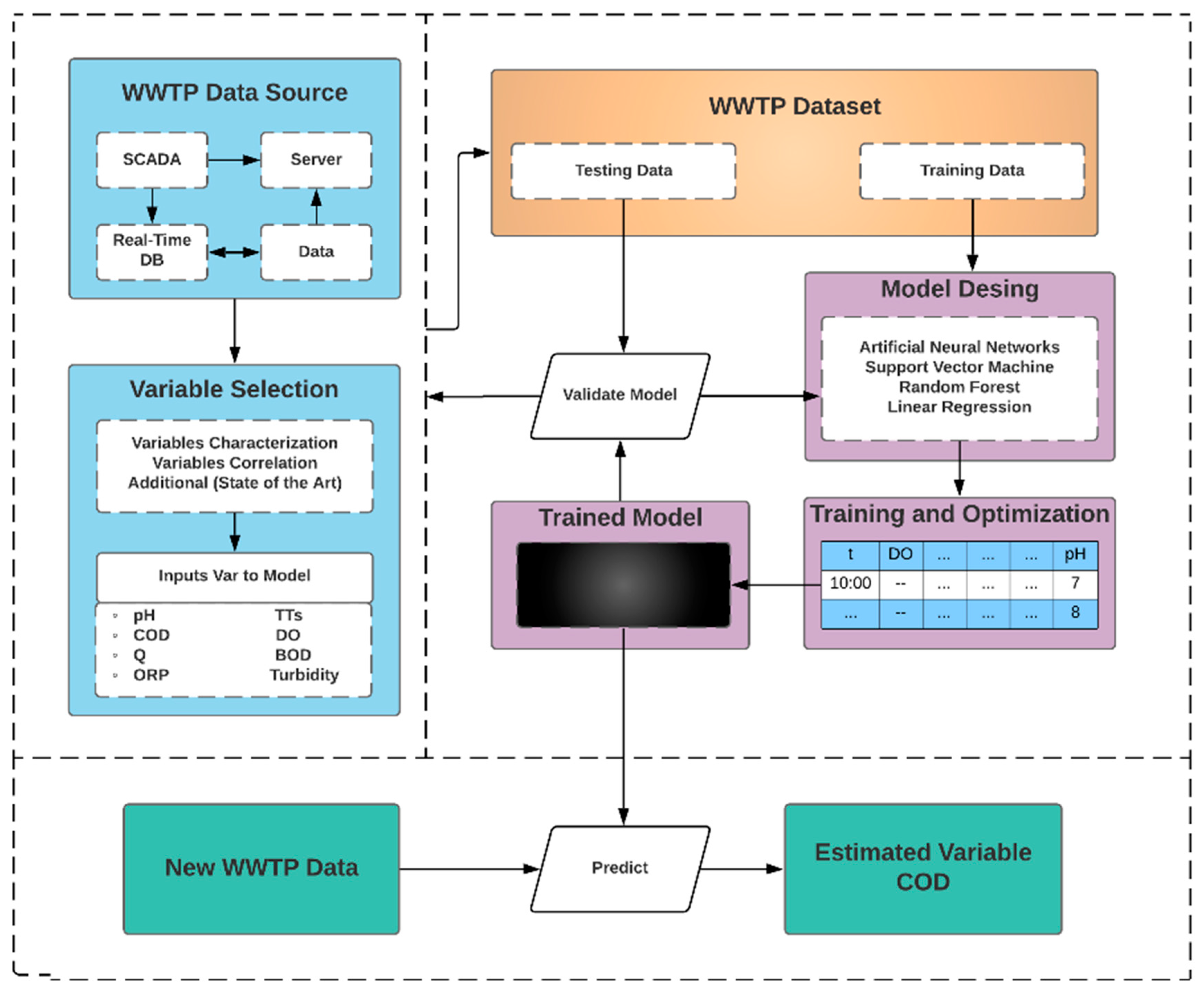
3.1. Model Design

COD is one of the most important variables in the process of a biological treatment since experts can make decisions based on the measurements of this variable. The objective of biological wastewater treatment is to perform a system to remove the pollutants present in water. Thus, this treatment is used overall because it is compelling and more efficient than numerous mechanical or compound procedures. In the bioreactor at this stage, a variety of microorganisms are used to break down organic matter in the water. However, the microorganisms are susceptible to change, depending on all the conditions in the tank.
For this reason, the present work proposes to use predictive analysis on COD to make decisions, knowing how contaminated the water will be in the tank. For studying how COD dynamics in the process are, a dataset was received from a WWTP from the Nantong, China plant with a daily data frequency for a total of 847 samples at different stages of the process, where a total of 22 variables were collected from 01/12/2017 to 24/05/2020. The COD dynamic can be observed in Figure 2.
Figure 3 shows the biological stages of the process in which the organic load of water is removed. Some important variables for the project that describe the WWTP process are represented as circles in blue and green. The blue circle is the output variable COD for the forecasting analysis, while green circles are input variables to design the intelligent system.
For the development of the system, the selected technology was an ANN because of the state-of-the-art review supported by the complexity of the WWTP process. Figure 4 presents the flowchart that synthesizes the design process of the intelligent systems proposed, which started with the data collection and the use of different strategies for variable selection. Within the dataset, the main variables of the process were:
  • Flow
  • COD of influent water
  • Suspended solids in influent water (SS)
  • Mixed liquor suspended solids (MLSS)
  • Mixed liquor volatile suspended solids (MLVSS)
  • Nitrogen (N)
  • pH
  • Mixed liquor dissolved oxygen (DO)
  • Food to microorganism (F/M)
Each characteristic can be repeated in one or more stages that are listed as below:
  • EQ = Equalizer
  • BIO = Bioreactor
  • BT_N = Bioreactor Pit N
  • BT_C = Bioreactor Pit C
  • Clari = Clarifier
  • OxT = Oxidation Tank
  • D = Discharge Pit
After variable selection, the dataset is split into training, validation and test sets. However, in this case, the data was split into training and test sets since the number of samples was small in comparison with the amount of data used to train an ANN. It is important to note that a computational technique must be selected. As mentioned before in related works in Table 3, about 64.71% of the work of authors used an algorithm from the ANN group to develop forecast models. It has been verified that neural networks have suitable results in the area since the water treatment process is characterized by being nonlinear in behavior, so if they are used properly, they can represent the dynamics of this process very well. Once the model was selected, the model was trained and brought into operating condition to estimate COD. An error measure is necessary to support the performance of the model. Therefore, the MAPE), defined as shown in Equation (1), was chosen to quantify the ANN error. In this equation, x i represents the actual point, which is intended to be predicted, x ^ i represents the predicted values of that observed point and N is the number of observed values that are intended to be predicted.
MAPE   = 100 N i = 1 N | x i x ^ i x i | ,
Figure 5 shows in more detail how the model is conceived and how the COD forecasting is achieved. First, the objective variable taken from the dataset is studied using a time-series decomposition technique that transforms the variable into three additive components: trend, seasonality and residual. Leveraging an autocorrelation study over the components, the first two are estimated using their past values. On the other hand, the residual component is estimated using an ANN, which received exogenous variables selected from a correlation study and a past value of the same component. Finally, the addition of the three components provides the COD prediction. All data analysis and the intelligent system training were carried out by using Python, mainly taking advantage of Pandas, NumPy, Matplotlib, Statsmodels and TensorFlow libraries.

3.2. Platform Design

A web platform was designed to visualize all the variables of the WWTP dynamically, monitor the COD prediction provided by the forecast model and consult the historical measurements of the variables. Thus, the main sections of the platform were built as the real-time and historical data view. For this purpose, a model–view–controller schema was used to construct the platform using the technologies as Figure 6 shows. The technology that performed the view in the platform was ReactJS, responsible for rendering the visual content to interact with the user and make requests (frontend). ReactJS related to the master and brain of the platform, NodeJS, which controlled the logic responsible for managing all functions and methods that made the platform work (backend). Parallelly with NodeJS, TensorFlow.JS deployed the trained forecast model, which was developed to predict the COD at the beginning of the bioreactor. Besides, all the data and the information important to be the cog in this system were stored in a database schema settled in PostgreSQL. The interaction between those technologies allowed for reaching the objectives mentioned.

4. Results

The experiments carried out were time-series decomposition, autocorrelation study and correlation study. Each one was to get the best performance of the model described below.

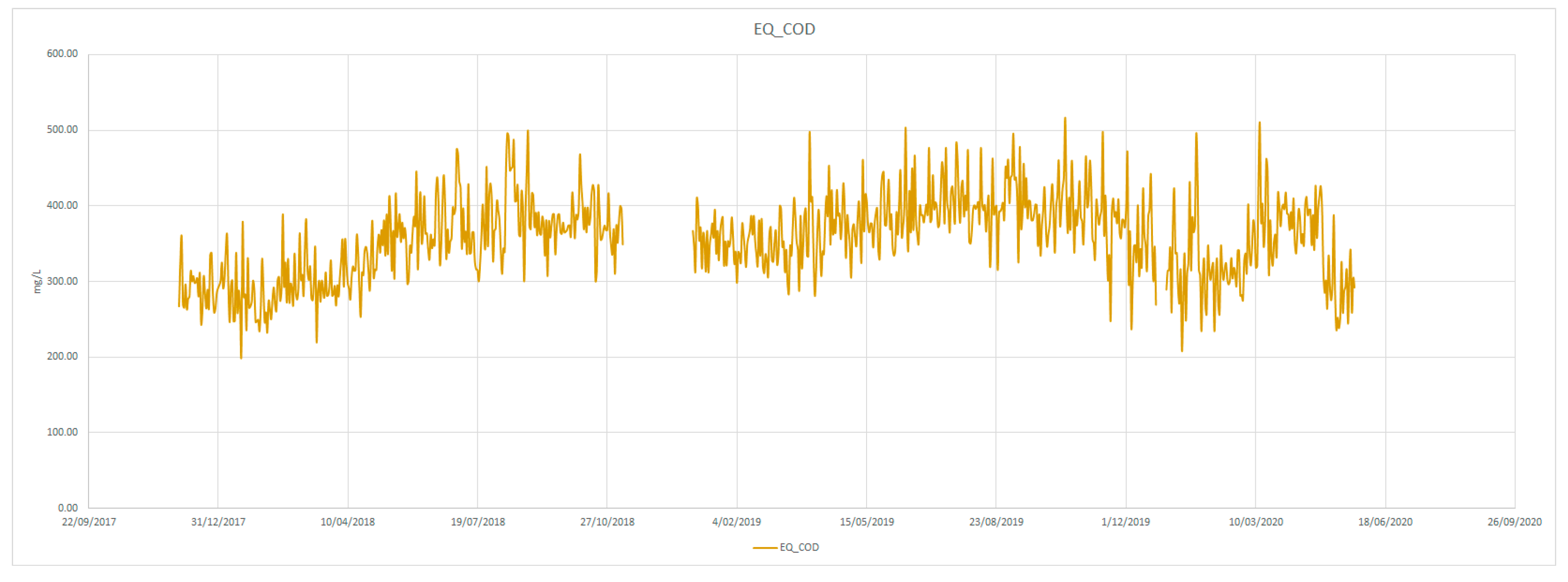
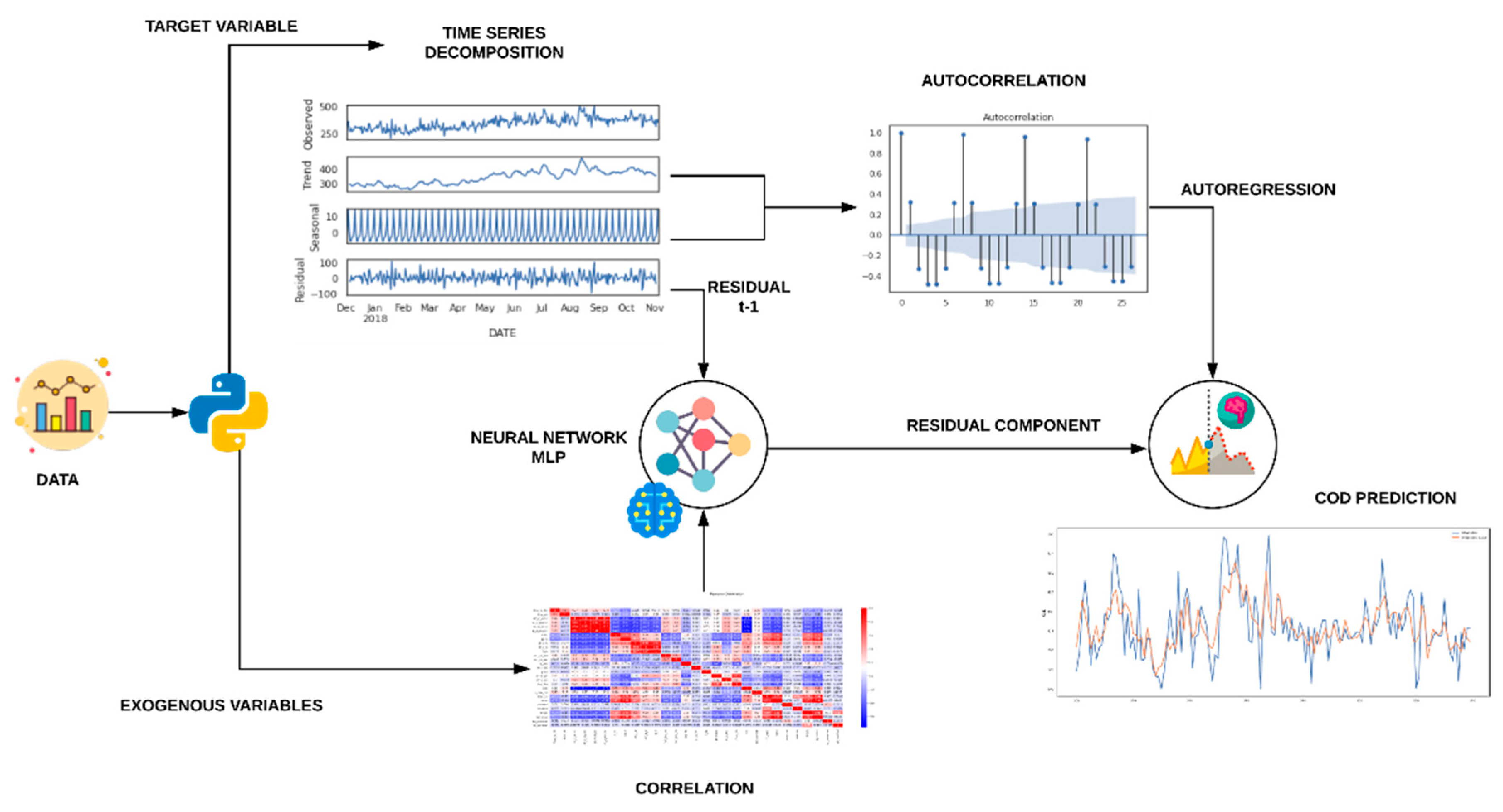
4.1. Time-Series Decomposition

For the time-series analysis of the target, the variable was made a component decomposition where the time series could be represented as a combination of trend, seasonality and residual components [35]. From this point, it was intended to forecast each component of the time series to obtain the objective series using the additive model stated by Pearson and presented in Equation (2) [36], where Tt refers to tendency or trend, St to seasonal movements, Rt to residuals or irregulars and Xt to the series observed.
Xt = Tt + St + Rt,
Figure 7 shows an example of how the equalizer’s COD decomposition looks for the year 2019, where (a) shows the original COD variable, (b) the trend component, (c) the seasonal component and (d) the residual component.

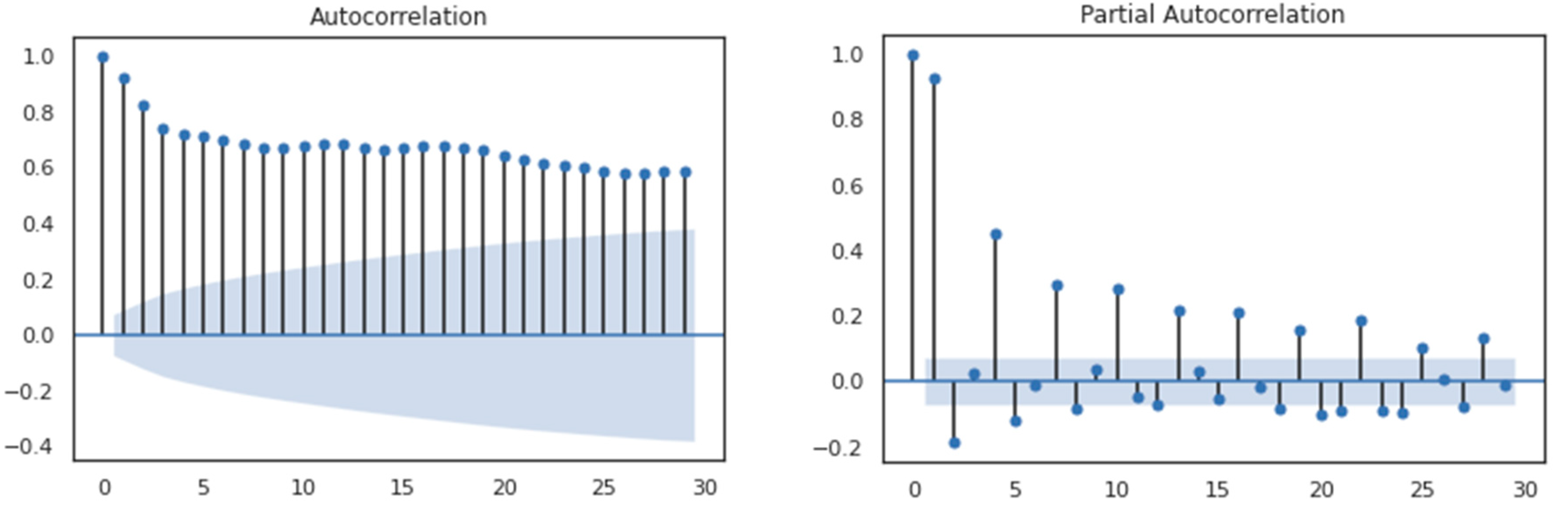
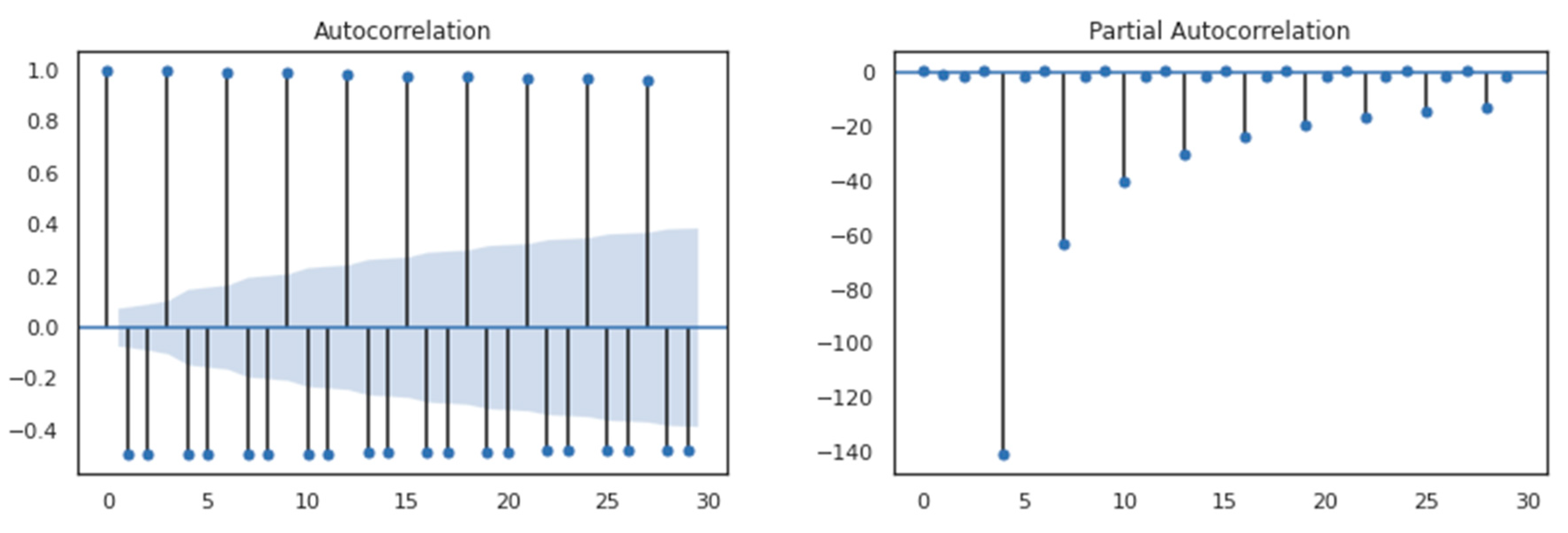
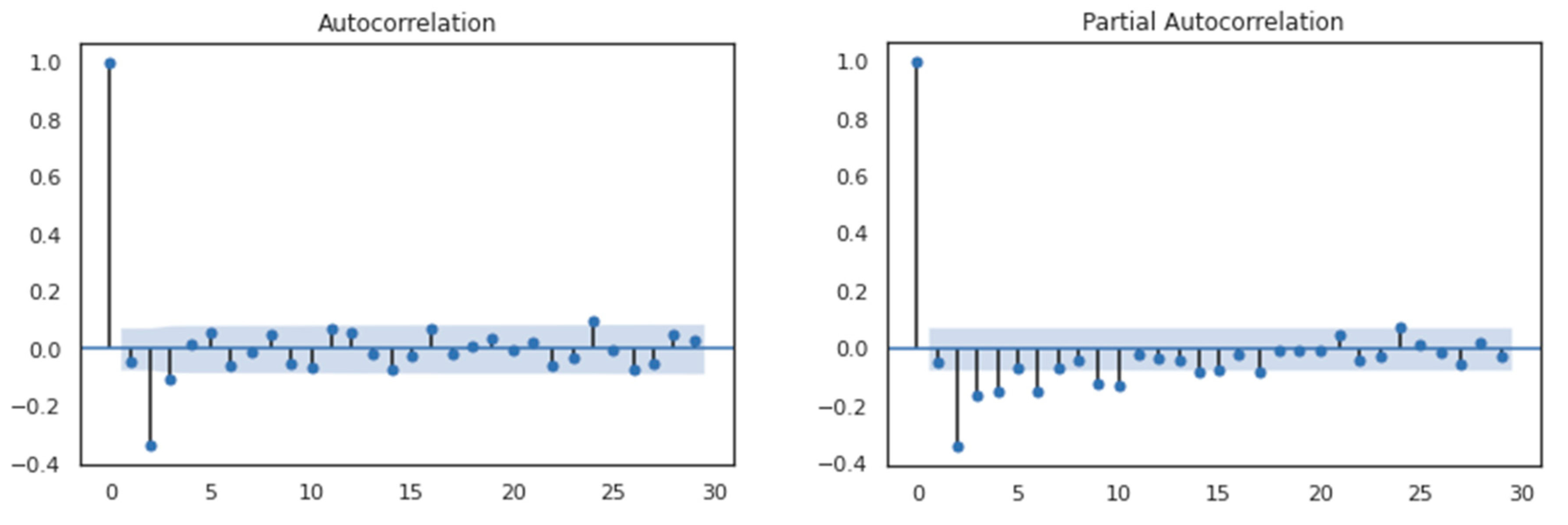
4.2. Autocorrelation Study

Analyzing the time-series decomposition, both autocorrelation and partial autocorrelation studies were made on residual, seasonal and trend COD to extract the important characteristics. From this analysis, it was possible to conduct an autoregressive estimation of the trend and seasonal component of the series. Figure 8, Figure 9 and Figure 10 show the total and partial autocorrelation, respectively.
From Figure 8, it is clear how the past values were strongly correlated with the current COD trend value. Thus, the trend record provided significant information to the model on the dynamics of the COD. Additionally, Figure 9 shows the important effect of the seven past seasonal values. On the other hand, for the COD residual autocorrelation, the analysis was not very revealing, but it can be highlighted that for data with a validity of two days, there was a correlation of almost −0.35 with the current COD value.

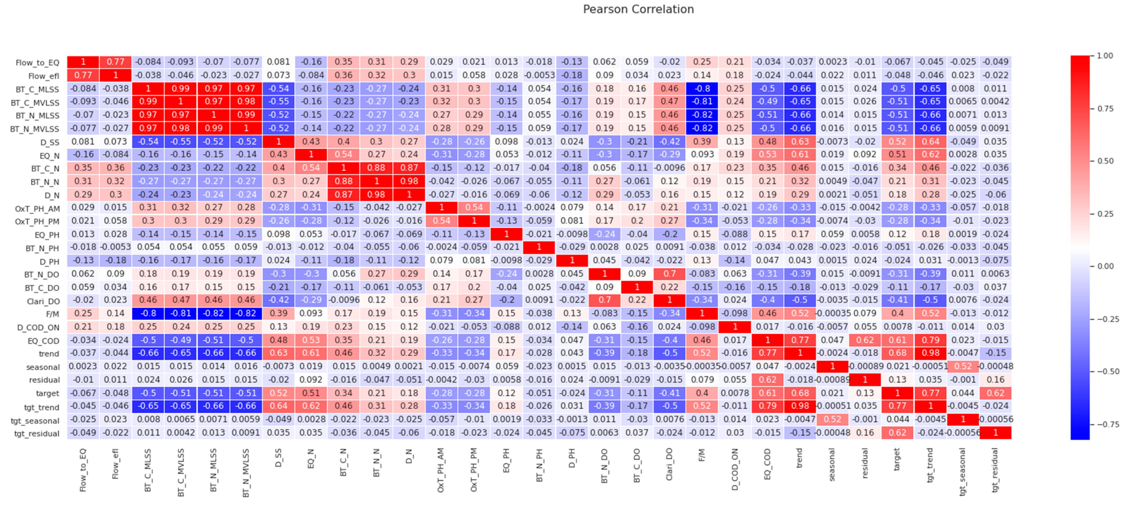
4.3. Correlation Study

For determining which variables had a significant effect on the COD dynamic, a correlation study was used to decant characteristics and reduce the dimensionality of the model. Thus, the model could learn without the noise caused by raw characteristics. Besides, the variables with a high correlation improved system performance. The correlation selected for the analysis was the Pearson correlation since when exploring other types of correlations, the results were similar. The correlation results were carried out using the variable EQ_COD a day ahead of the target, considering that this was the purpose of this job. Figure 11 shows the correlation matrix, and focusing on the target, the suggested exogenous variables are below:
  • BT_C_MLVSS
  • D_SS
  • BT_C_N
  • EQ_N
  • Clari_DO
  • F/M
Table 4 shows the correlation analysis summary focused on the target variable. To be noted, the selection threshold for the correlation was adjusted to 0.4, thus obtaining most of the variables suggested by the experts in the study area. However, BT_C_MLSS, BT_C_MLVSS, BT_N_MLSS and BT_N_MLVSS were highly related; therefore, the set could be represented by a single variable. In this case, BT_C_MLSS was selected, but any of the rest could be chosen. It is worth highlighting that EQ_COD on the correlation table refers to the current value of the variable.

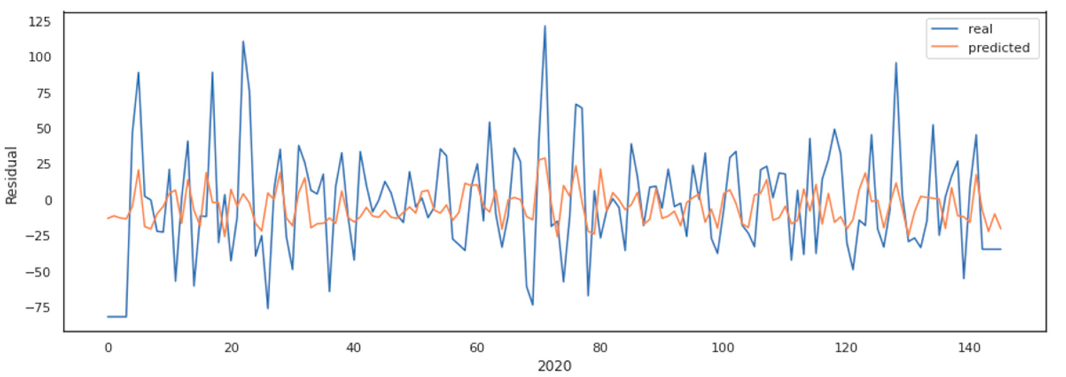
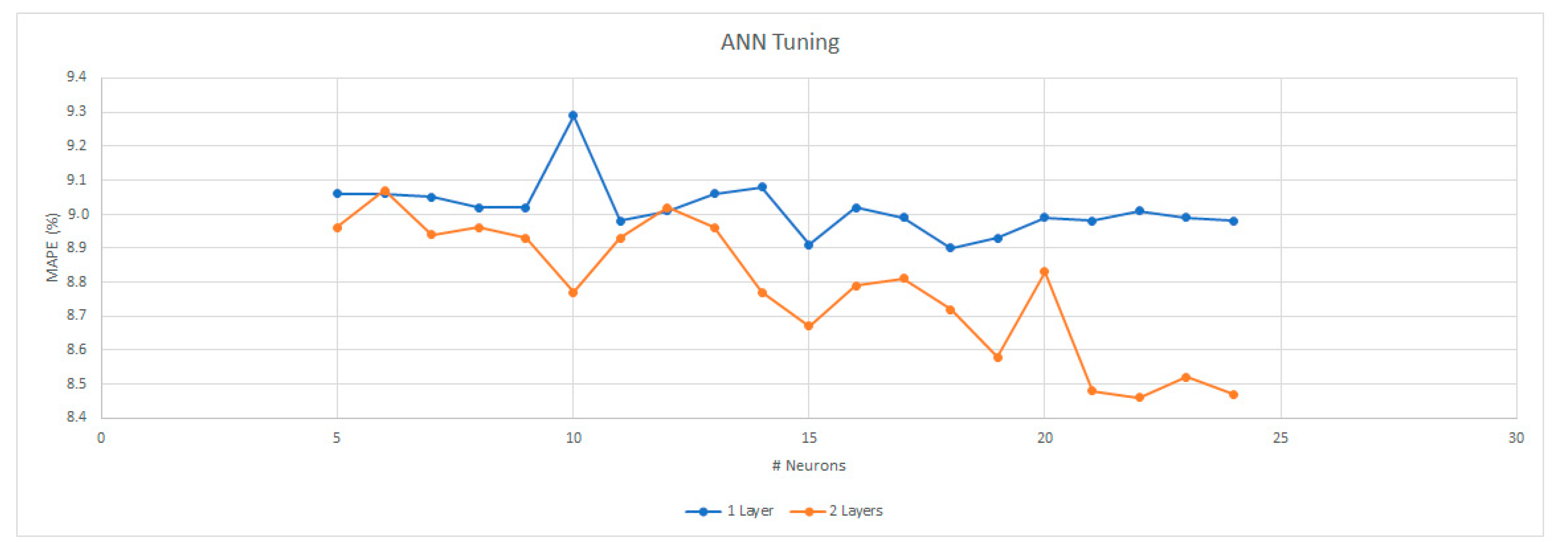
4.4. Artificial Neural Network
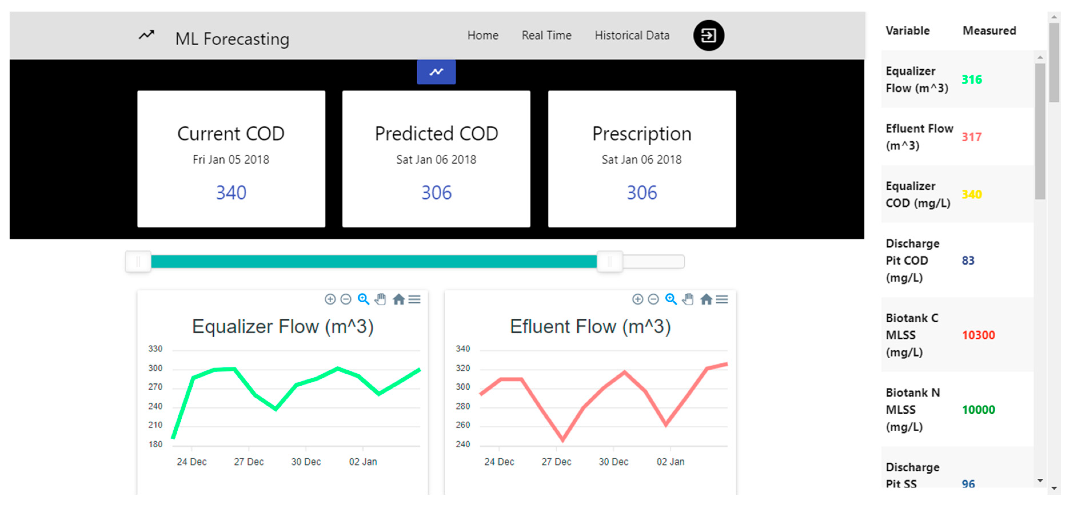
Utilizing selected variables from the correlation study, an artificial neural network was implemented to forecast the time-series residual. The architecture implemented was a multilayer perceptron (MLP) fully connected with 7 neurons in the input layer and 2 hidden layers, with 22 neurons each, and 1 neuron in the output layer to predict the residual component. The neural network was trained with approximately 80% of the samples, and 147 corresponding samples from the year 2020 were used for the test. During the 150 training periods, the training used the backpropagation algorithm to update the weights in the neurons, with the mean square error (MSE) as the loss function and Adam optimizer. Figure 12 shows the preliminary results, where the blue series is the real one and the orange is the predicted value.
The number of neurons in each hidden layer of the neural network was obtained through a grid search, as shown in Figure 13, using training data.
Using the autoregressive estimation conducted on the trend, seasonal and the residual component obtained by the ANN, it was possible to forecast the equalizer COD (adding together the three components) as shown in Figure 14, obtaining a MAPE of 10.8%, which is appropriate with the values found in the literature, where similar works reported MAPEs between 4% and 11% as good forecasting performance.
The prediction achieved and presented above was made day by day, as was the error obtained. Pikes on the COD dynamic were not reached by the model. However, it was considered to increase the number of samples to improve the performance of the model in future work.

4.5. Web Platform.

The final result of the platform was designed so that a user could visualize all the variables of the WWTP dynamically, monitor the COD prediction and check the historical measurements of the variables (see Figure 15).
This section hides a powerful backend behind its interface. The box where the current COD is displayed responds to the measurement that is currently being read from the COD variable at that moment. The box titled as Predicted COD is directly connected to the model that gives a prediction in response to the current COD input and the selected exogenous variables. To compare the behavior between the real and predicted COD, a window is available, as Figure 16 shows (this figure captured only behavior with training data). The prescription box is thought of and built for future work. On the other hand, there is a visualization of all the process variables and a condensed summary in a table of the measurement of each variable.
To have a visualization of the historical data, a section was developed with the corresponding graphs and a summary table to be able to choose a historical data point from the graphs and detail it in the right table. Figure 17 shows this result.

5. Discussion

The selection and characterization of the most significant variables of the wastewater treatment process have been carried out satisfactorily using correlation analysis, autocorrelations and decomposition of the time series. With these variables, an intelligent system based on artificial neural networks was developed to be capable of giving an adequate prediction of chemical oxygen demand, one of the most suitable variables to measure the level of pollutant load in the water and make decisions. The results show that the model presented a MAPE of 10.8%, which supports its good performance according to historical data mentioned in [14], where the testing step ranged between 10% and 13%, predicting BOD, COD or TSS. Additionally, it is worth mentioning that this work presents as a novelty the use of time-series decomposition techniques to address the COD prediction and using an ANN, in comparison with the works presented in Section 2, whose summary can be seen in Table 2. This methodology can be useful to improve the prediction of some complex variables in which the ANNs do not have the desired performance. Finally, a platform was possible to design mainly to visualize available WWTP variables, monitor COD forecasting and consult the historical measurements.
In search of constant improvement of the industrial wastewater treatment process, it is considered for future works to scale the prediction of the system to other key variables of the process, obtain a larger amount of data considering newly available measurements in the process and increase the scope of the prediction.

Author Contributions

Conceptualization, A.M. and R.M.; methodology, C.G.Q.M.; software, L.A. and C.C.; validation, L.A., C.C. and C.G.Q.M.; formal analysis, L.A., C.C. and C.G.Q.M.; investigation, L.A., C.C. and C.G.Q.M.; resources, D.G.; data curation, L.A. and C.C.; writing—original draft preparation, L.A. and C.C.; writing—review and editing, L.A., C.C., D.G., A.M., R.M. and C.G.Q.M.; visualization, L.A. and C.C.; supervision, C.G.Q.M.; project administration, D.G.; funding acquisition, D.G. All authors have read and agreed to the published version of the manuscript.

Funding

This research was supported by the Colombian Ministry of Science and Technology, MINCIENCIAS, Investment Tax Benefits, Call No. 786.

Acknowledgments

This work was supported by the Universidad del Norte, Barranquilla, Colombia.

Conflicts of Interest

The authors declare that there are no conflict of interest regarding the publication of this paper.

Abbreviations

AbbreviationDefinition
ANFISAdaptive neuro-fuzzy inference system
ANNArtificial neural network
BNBayesian network
BPBackpropagation network
CODChemical oxygen demand
DCDetermination coefficient
DTDecision tree
drelRelative efficiency criteria
ELMExtreme learning machine
F/MFood to microorganism
FFNNFeedforward neural network
FLFuzzy logic
FNNFuzzy neural network
GAGenetic algorithm
GNDGaussian naive Bayes
GRIGlobal Reporting Initiative
HRTHydraulic retention time
ICSImproved cuckoo search
IPWIterative predictor weighting
KNNK-nearest neighbors
MAPEMean absolute percentage error
MLPANNMultilayer perceptron ANN
MLRMultilinear regression
MSEMean square error
MLSSMixed liquor suspended solids
MLVSSMixed liquor volatile suspended solids
NARXMultivariate nonlinear autoregressive exogenous
NFCNeuro-fuzzy controller
NH4-NAmmonium
NSENash–Sutcliffe efficiency
O&GOil and grease
PCAPrincipal component analysis
PCCPearson correlation coefficient
PLSPartial least squares
QLQ-learning
RCorrelation coefficient
R2Coefficient of determination
RBFANNRadial basis function ANN
RFRandom forest
RMSERoot mean square error
RMSEPRoot mean squared error of prediction
SCFLSupervised committee FL
SOMSelf-organizing maps
SRMStructural risk minimization
SVISludge volume index
SVMSupport vector machine
TNTotal nitrogen
TPTotal phosphorus
TSSTotal suspended solids
UVEUninformative variable elimination
WWTPWastewater treatment plant

References

  1. UNWWA Programme. The United Nations World Water Development Report 3: Water in a Changing World; UNESCO: Paris, France, 2008. [Google Scholar]
  2. Sener, E.S.S.; Devraz, A. Evaluation of water quality using water quality index (WQI) method and GIS in Aksu River (SW-Turkey). Sci. Total Environ. 2017, 584–585, 131–144. [Google Scholar] [CrossRef] [PubMed]
  3. Newhart, K.B.; Holloway, R.W.; Hering, A.S.; Cath, T.Y. Data-driven performance analyses of wastewater treatment plants: A review. Water Res. 2019, 157, 498–513. [Google Scholar] [PubMed]
  4. Anjun, M.; Al-Makishah, N.H.; Barakat, M.A. Wastewater sludge stabilization using pre-treatment methods. Proc. Saf. Environ. Prot. 2016, 102, 615–632. [Google Scholar] [CrossRef]
  5. Tchobanoglous, G.; Schroeder, E.E. Water Quality: Characteristics, Modeling, Modification; Addison-Wesley Publishing Company: Boston, MA, USA, 1985. [Google Scholar]
  6. Lake, B.M.; Ullman, T.D.; Tenebaum, J.B.; Gershman, S.J. Building machines that learn and think like people. Behav. Brain Sci. 2017, 40, e253. [Google Scholar] [CrossRef] [Green Version]
  7. V´ıtez, J.S.T.; Oppeltov´a, P. Evaluation of the efficiency of selected wastewater treatment plant. Acta Univ. Agric. Silvic. Mendel. Brun. 2012, 60, 173–180. [Google Scholar] [CrossRef] [Green Version]
  8. Romero, J.M.P.; Hallet, S.H.; Jude, S. Leveraging big data tools and technologies: Addressing the challenges of the water quality sector. Sustainability 2017, 9, 12. [Google Scholar]
  9. Sbroiavacca, A.; Sbroiavacca, F. Industry 4.0: The Exploitation of Big Data and Forthcoming Perspectives, Economic and Social Development. In Book of Proceedings, Proceedings of the 35thInternational Scientific Conference on Economic and Social Development–Sustainability from an Economic and Social Perspective, Lisbon, Portugal, 15–16 November 2018; ESD Publishing: Varazdin, Croatia, 2018; pp. 742–745. [Google Scholar]
  10. Nourani, V.; Elkiran, G.; Abba, S.I. Wastewater treatment plant performance analysis using artificial intelligence—An ensemble approach. Water Sci. Technol. 2018, 78, 2064–2076. [Google Scholar] [CrossRef]
  11. Pang, J.; Yang, S.; He, L.; Chen, Y.; Ren, N. Intelligent control/operational strategies in WWTPs through an integrated Q-learning algorithm with ASM2d-guided reward. Water 2019, 11, 927. [Google Scholar] [CrossRef] [Green Version]
  12. Li, D.; Yang, H.Z.; Liang, X.F. Prediction analysis of a wastewater treatment system using a Bayesian network. Environ. Model.Softw. 2013, 40, 140–150. [Google Scholar] [CrossRef]
  13. Haggege, J.; Benrejeb, M.; Borne, P. On the design of a neuro-fuzzy controller—Application to the control of a bioreactor. J. Syst. Sci. Syst. Eng. 2005, 14, 417–435. [Google Scholar] [CrossRef]
  14. Nadiri, A.A.; Shokri, S.; Tsai, F.T.; Asghari Moghaddam, A. Prediction of effluent quality parameters of a wastewater treatment plant using a supervised committee fuzzy logic model. J. Clean. Prod. 2018, 180, 539–549. [Google Scholar] [CrossRef]
  15. Han, H.; Zhu, S.; Qiao, J.; Guo, M. Data-driven intelligent monitoring system for key variables in wastewater treatment process. Chin. J. Chem. Eng. 2018, 26, 2093–2101. [Google Scholar] [CrossRef]
  16. Guo, H.; Jeong, K.; Lim, J.; Jo, J.; Kim, Y.M.; Park, J.-P.; Kim, J.H.; Cho, K.H. Prediction of effluent concentration in a wastewater treatment plant using machine learning models. J. Environ. Sci. 2015, 32, 90–101. [Google Scholar] [CrossRef]
  17. Alsina, E.F.; Chica, M.; Trawiński, K.; Regattieri, A. On the use of machine learning methods to predict component reliability from data-driven industrial case studies. Int. J. Adv. Manuf. Technol. 2018, 5, 2419–2433. [Google Scholar] [CrossRef]
  18. Dairi, A.; Cheng, T.; Harrou, F.; Sun, Y.; Leiknes, T. Deep learning approach for sustainable WWTP operation: A case study on data-driven influent conditions monitoring. Sustain. Cities Soc. 2019, 50, 101670. [Google Scholar] [CrossRef]
  19. Bagheri, M.; Mirbagheri, S.A.; Bagheri, Z.; Kamarkhani, A.M. Modeling and optimization of activated sludge bulking for a real wastewater treatment plant using hybrid artificial neural networks-genetic algorithm approach. Proc. Saf. Environ. Prot. 2015, 95, 12–25. [Google Scholar] [CrossRef]
  20. Ráduly, B.; Gernaey, K.V.; Capodaglio, A.; Mikkelsen, P.S.; Henze, M. Artificial neural networks for rapid WWTP performance evaluation: Methodology and case study. Environ. Model. Softw. 2007, 22, 1208–1216. [Google Scholar] [CrossRef]
  21. Liukkonen, M.; Laakso, I.; Hiltunen, Y. Advanced monitoring platform for industrial wastewater treatment: Multivariable approach using the self-organizing map. Environ. Model. Softw. 2013, 48, 193–201. [Google Scholar] [CrossRef]
  22. Jimenez, J.; Latrille, E.; Harmand, J.; Robles, Á.; Ferrer, J.; Gaida, D.; Wolf, C.; Mairet, F.; Bernard, O.; Alcaraz-González, V.; et al. Instrumentation and control of anaerobic digestion processes: A review and some research challenges. Rev. Environ. Sci. Biotechnol. 2015, 14, 615–648. [Google Scholar] [CrossRef]
  23. Reis, M.; Gins, G. Industrial Process Monitoring in the Big Data/Industry 4.0 Era: From Detection, to Diagnosis, to Prognosis. Process 2017, 5, 35. [Google Scholar] [CrossRef] [Green Version]
  24. Zounemat-Kermani, M.; Stephan, D.; Hinkelmann, R. Multivariate NARX neural network in prediction gaseous emissions within the influent chamber of wastewater treatment plants. Atmospheric Pollut. Res. 2019, 10, 1812–1822. [Google Scholar] [CrossRef]
  25. Yu, P.; Cao, J.; Jegatheesan, V.; Du, X. A Real-time BOD Estimation Method in Wastewater Treatment Process Based on an Optimized Extreme Learning Machine. Appl. Sci. 2019, 9, 523. [Google Scholar] [CrossRef] [Green Version]
  26. Ye, Z.; Yang, J.; Zhong, N.; Tu, X.; Jia, J.; Wang, J. Tackling environmental challenges in pollution controls using artificial intelligence: A review. Sci. Total Environ. 2020, 699, 134279. [Google Scholar] [CrossRef]
  27. Hernández-Del-Olmo, F.; Gaudioso, E.; Duro, N.; Dormido, R. Machine Learning Weather Soft-Sensor for Advanced Control of Wastewater Treatment Plants. Sensors 2019, 19, 3139. [Google Scholar] [CrossRef] [PubMed] [Green Version]
  28. Sangüesa, R.; Burrell, P. Application of Bayesian Network Learning Methods to Waste Water Treatment Plants. Appl. Intell. 2000, 13, 19–40. [Google Scholar] [CrossRef]
  29. Qin, X.; Gao, F.; Chen, G. Wastewater quality monitoring system using sensor fusion and machine learning techniques. Water Res. 2012, 46, 1133–1144. [Google Scholar] [CrossRef]
  30. Dellana, S.; West, D. Predictive modeling for wastewater applications: Linear and nonlinear approaches. Environ. Model. Softw. 2009, 24, 96–106. [Google Scholar] [CrossRef]
  31. Alsina, E.F.; Cabri, G.; Regattieri, A. A neural network approach to find the cumulative failure distribution: Modeling and experimental evidence. Qual. Reliab. Eng. Int. 2016, 32, 567–579. [Google Scholar] [CrossRef]
  32. Siddiqui, T.; Al Kadri, M. Big data analytics on the cloud. Int. J. Emerg. Technol. Comput. Appl. Sci. (IJETCAS) 2015, 24, 61–66. [Google Scholar]
  33. Siddiqui, T.; Al Kadri, M.; Khan, N.A. Review of programming languages and tools for big data analytics. Int. J. Adv. Res. Comput. Sci. 2017, 8, 1112–1118. [Google Scholar]
  34. Valentín-Vargas, A.; Toro-Labrador, G.; Massol-Deyá, A.A. Bacterial community dynamics in full-scale activated sludge bioreactors: Operational and ecological factors driving community assembly and performance. PLoS ONE 2012, 7, e42524. [Google Scholar] [CrossRef] [PubMed] [Green Version]
  35. Cryer, J.D.; Chan, K.-S. Time Series Analysis; Springer: New York, NY, USA, 2008. [Google Scholar]
  36. Dagum, E. Time series modelling and decomposition. Statistica 2013, 70, 5. [Google Scholar]
Figure 1. SAS, R or Python preferences.
Sustainability 12 06348 g001
Figure 2. Chemical oxygen demand behavior.
Sustainability 12 06348 g002
Figure 3. Biological WWTP process diagram.
Sustainability 12 06348 g003
Figure 4. Model structure diagram.
Sustainability 12 06348 g004
Figure 5. Model block diagram.
Sustainability 12 06348 g005
Figure 6. Platform schema.
Sustainability 12 06348 g006
Figure 7. Equalizer chemical oxygen demand (COD) decomposition.
Sustainability 12 06348 g007
Figure 8. COD trend analysis correlation.
Sustainability 12 06348 g008
Figure 9. COD seasonal analysis correlation.
Sustainability 12 06348 g009
Figure 10. COD residual analysis correlation.
Sustainability 12 06348 g010
Figure 11. Correlation matrix.
Sustainability 12 06348 g011
Figure 12. Residual prediction.
Sustainability 12 06348 g012
Figure 13. Artificial neural network (ANN) tuning.
Sustainability 12 06348 g013
Figure 14. COD prediction.
Sustainability 12 06348 g014
Figure 15. Real-time view.
Sustainability 12 06348 g015
Figure 16. COD monitoring.
Sustainability 12 06348 g016
Figure 17. Historical data view.
Sustainability 12 06348 g017
Table 1. Big data tools.
AreaAmazonMicrosoftGoogle
Big data storageS3AzureGoogle Cloud services
Big data analyticsElastic MapReduce (Hadoop)Hadoop on AzureBigQuery
Relational database MySQL or OracleSQL AzureCloud SQL
NoSQL databaseDynamoDBTable storageApp Engine Datastore
MapReduceElastic MapReduce (Hadoop)Hadoop on AzureApp Engine
Streaming processingNothing prepackagedStreamInsightSearch API
Machine learningHadoop + MahoutHadoop + MahoutPrediction API
Data sourcesPublic datasetsWindows Azure marketplaceA few sample datasets
AvailabilityPublic productionSome services in private betaSome services in private beta
Table 2. Related works.
RefYearMethodPredictionError
[10]2018FFNN, ANFIS, SVM, MLRBOD, COD, TNDC, RMSE
[11]2019Q-learning--
[12]2012Bayesian networkCOD, TP, TN-
[13]2005NFCDilution rate-
[14]2018FL, SCFL, ANNBOD, COD, TSSMAPE
[15]2018FNN, PCABOD, COD, TSS, TP, NH4-N-
[16]2015ANN, SVMTP, TSS, CODR2, NSE, drel
[19]2015
MLPANN–GA,
RBFANN–GA
SVI-
[20]2006ANNBOD, COD, TSS, TNR2
[21]2013SOM--
[24]2019NARXH2S emissionMAPE, RMSE, GRI
[25]2019ICS–ELM, BPBOD-
[29]2012PLS, IPW–PLS,
Boosting-IPW–PLS
COD, TSS, NTUMinE, RMSEP, MaxE, R
[34]2012-BOD, TSS, HRT, F/M-
Table 3. Computational techniques used in wastewater treatment plant (WWTP) analysis from related works.
Algorithm%Algorithm%
ANN64.71KNN5.88
SVM23.53PCA5.88
Fuzzy17.65PLS5.88
BN11.76QL5.88
RF11.76GND5.88
DT5.88ICS5.88
Table 4. Correlation analysis summary.
VariableValue
Flow_to_EQ0.067
Flow_efl0.048
BT_C_MLSS0.50
BT_C_MLVSS0.51
BT_N_MLSS0.51
BT_N_MLVSS0.51
D_SS0.52
EQ_N0.51
BT_C_N0.34
BT_N_N0.21
D_N0.18
OxT_pH Morning0.28
OxT_pH Afternoon0.28
EQ_pH0.12
BT_N_pH0.051
D_pH0.024
BT_N_DO0.31
BT_C_DO0.11
Clari_DO0.41
F/M0.40
D_COD_ON0.0078
EQ_COD (t)0.61

