Machine Learning Application in Reservoir Water Level Forecasting for Sustainable Hydropower Generation Strategy

Abstract

The aim of this study is to accurately forecast the changes in water level of a reservoir located in Malaysia with two different scenarios; Scenario 1 (SC1) includes rainfall and water level as input and Scenario 2 (SC2) includes rainfall, water level, and sent out. Different time horizons (one day ahead to seven days) will be investigated to check the accuracy of the proposed models. In this study, four supervised machine learning algorithms for both scenarios were proposed such as Boosted Decision Tree Regression (BDTR), Decision Forest Regression (DFR), Bayesian Linear Regression (BLR) and Neural Network Regression (NNR). Eighty percent of the total data were used for training the datasets while 20% for the dataset used for testing. The models’ performance is evaluated using five statistical indexes; the Correlation Coefficient (R²), Mean Absolute Error (MAE), Root Mean Square Error (RMSE), Relative Absolute Error (RAE), and Relative Squared Error (RSE). The findings showed that among the four proposed models, the BLR model outperformed other models with R² 0.998952 (1-day ahead) for SC1 and BDTR for SC2 with R² 0.99992 (1-day ahead). With regards to the uncertainty analysis, 95PPU and d-factors were adopted to measure the uncertainties of the best models (BLR and BDTR). The results showed the value of 95PPU for both models in both scenarios (SC1 and SC2) fall into the range between 80% to 100%. As for the d-factor, all values in SC1 and SC2 fall below one.

1. Introduction

A reservoir is a physical structure (artificial and natural) used as water storage for water storage preservation, control, and regulation of water supply [1]. Thus, climate change is likely to cause parts of the reservoir’s water cycle to intensify as warming global temperatures increase the rate of evaporation around the world. More evaporation is causing more precipitation on average where it leads to increasing of water level in reservoir. When a reservoir is full at the top water level because of excessive inflow, it will cause the water level to rise and increase the rates of discharge over the spillway. This event can cause flooding downstream. Flooding is one of the extreme events that has a major impact on reservoirs, especially at unregulated sites where it can directly or indirectly cause extreme losses to the public such as houses, facilities, assets, or innocent souls [2]. The water level in all water bodies changes to some extent and the intake facility should be considered in terms of the anticipated varieties. During drought season, the water level in reservoirs will be low and abstraction might not be permitted. Though the abstraction is permitted, the water level may still not be high enough to drive the desired stream into the intake. A weir or torrent may be required to sustain an adequate water level. One major problem in current dam impact studies is the lack of a reliable model for simulating the implications of water level on the reservoir operation. It reduces the efficiency of the reservoir operation as some amount of water has to be released through the spillway to ensure the water level is below the full supply level. In forecasting reservoir water levels, two methods can be applied, which is to weigh the model utilizing the water level’s natural factors and to acknowledge the natural factors effecting historical water level to anticipate future levels [3]. Essentially, utilizing historical water level information can altogether diminish the inconsistency between factors in a model. Also, the importance of prior knowledge of water level will give benefit to the operator regarding the optimal draw of the water level and sustainable plan for hydropower generation. Therefore, this paper focuses on forecasting changes on water level using Machine Learning (ML) algorithms.

The term ML means to facilitate machines to review without programming them explicitly. In particular, the performance of ML in intelligence tasks is largely due to its ability to discover a complex structure that has not been defined prior [4]. There are four general ML methods [5,6]: (1) Supervised, (2) unsupervised, (3) semi-supervised, and (4) reinforcement learning methods. The difference between supervised and unsupervised learning is that supervised learning already has the expert knowledge to develop the input/output [7]. Meanwhile, unsupervised learning only has the input and the model will learn the hidden structure or data distribution to produce the output as cluster or feature [8,9,10]. The aim of ML is to allow machines to predict, cluster, extract association rules, or make decisions from a given dataset [11]. Over the past years, there has been numerous techniques employed in forecasting the hydrological events. Previously, the tools to forecast reservoir water level used conventional approach of linear mathematical relationships based on operator experience, mathematical curves, and guidelines [12]. However, due to the complexity and lack of access to the data, overestimating parameters and high missing values in data cause poor performances and undermining of numerical models. With regards to these issues, the use of ML approaches has been introduced, on the condition of improved results in modelling nonlinear processes and forecasting than traditional models, such as moving average methods [13,14,15]. The core advantage of this modelling is the skill of the software to plot the input–output patterns without the aforementioned expertise of the factors affecting the forecast parameters [16,17]. Hence, researchers have since started to practice this ML to predict variety of modelling approaches and parameters to improve the accuracy and reliability of describing the predicting model.

As such, numerous researchers used ML to forecast water level such as Artificial Neural Networks [18,19], Support Vector Machines (SVM) [17,19,20], Adaptive Neuro-Fuzzy Inference Systems (ANFIS) [17,18,19,20], Radial Basis Neural Networks (RBNN) [20], Generalized Regression Neural Networks (GRNN) [20], Radial Basis Function-Firefly Algorithm (RBF-FFA) [21], and Cuckoo Optimization Algorithms [18]. Furthermore, few researchers have also used hybrid and improvised models such as Wavelet-Based Artificial Neural Network (WANN) and Wavelet-Based Adaptive Neuro-Fuzzy Inference System (WANFIS) [22] and Least Squares Support Vector Machine (LSSVM) [23]. Damien [24] stated that all approaches of ML are within the same range as they all showed decent prediction in different scenarios and the quality of data used. However, the downside of using these ML techniques, such as ANN and ANFIS, is the outcome dissimilarity that depend on the complexity of the modeled system. Therefore, new ML approaches has been introduced in this study for forecasting the water level, which is Boosted Decision Tree Regression (BDTR). This BDTR has become more popular because of the simplicity of the model system. In spite of the simplicity, it can exhibit good predictive and tends to improve accuracy with minor risk of less coverage.

The major aim of the study is to provide the operator of the reservoir with accurate water level forecasting tool and investigate different modelling approaches like Boosted Decision Tree Regression (BDTR), Decision Forest Regression (DFR), Bayesian Linear Regression (BLR), and Neural Network Regression (NNR) and the effectiveness of these algorithms in learning the parameter pattern of water level. Secondly, the objective of this study is to assess and evaluate different scenarios and time horizons to find the most accurate and reliable model. Thirdly, this study is essential for industrial activities and progress, and better forecasting accuracy for water level would help generate better operation policies for the reservoir, which leads to better condition for water users including the business of agricultural process, industrial activities, and hydropower generation. As a result, the accurate forecasting for water level will positively affect for better planning for all related industrial and business activities. In a nutshell, the motivation of this study is necessary for predicting/forecasting the water level in the reservoir as it is an important variable for the decision-maker or the operator of the reservoir to know in order to be able to optimize the water resources planning.

2. Materials and Methods

2.1. Study Area and Dataset

Sultan Mahmud Power Station or Kenyir Dam is the Kenyir Lake, Terengganu, Malaysia hydroelectric dam and is situated 50 km in distance southwest of Kuala Terengganu (latitude: 5°1′25.23′′ N, longitude: 102°54′35.88′′ E) with catchment area is 1260 sq km. The Kenyir Reservoir was built by the structure of the Kenyir dam to sustain Sungai Terengganu flows throughout the year for the production of hydroelectric power. Figure 1 and Figure 2 illustrate the Kenyir Dam location and station layout.

Data for this study were secondary data, a total of 12,531 (34 years) historical data points were collected for the daily water level and daily rainfall from April 1985 to July 2019 and 82,057 (9 years) hourly sent out data from March 2010 to July 2019 were acquired from the Kenyir Operation Unit. For reservoir water level, the range was based on the hydraulic features of Kenyir Dam; minimum operating level was at 120 m, full supply level (FSL) was at 145 m, and the maximum water level was at 153 m. The basic statistical parameters, namely minimum, maximum, average, standard deviation (S.D.), and total count of the input are presented in

Table 1. Data acquired with descriptive statistics.

List of Data/Input	Unit	Minimum	Maximum	Average	S.D.	Count
Daily Water Level	mm	133.63	148.08	140.12	2.6385	12,531
Daily Rainfall	mm	0	1211	11.87	33.6455	12,531

.

2.2. Input Selection

In Machine Learning (ML), one of the main tasks is to choose input parameters that will influence output parameters because it will require attention and good understanding of the underlying physical process based on causal variables and statistical analysis of possible inputs and outputs [10]. Reservoir water level is basically affected by the hydrological phenomena such as rainfall, heat and temperature, evaporation, discharge, and also, the decision of send out water to the river downstream. Rising water level can cause flooding downstream and the importance of forecasting water level is to control the water release during dry and wet season.

There are two different input for forecasting water level, which are Scenario 1 (SC1) in Equation (1) and Scenario 2 (SC2) in Equation (2).

$$W{L}_{t+n}=R_t+W{L}_t$$

(1)

$$W{L}_{t+n}=W{L}_t+R_t+S_t$$

(2)

where $R_t$ is the rainfall and $W{L}_t$ is water level at time t and the water level for 7 days ahead, and where n is a day-ahead value like tomorrow until the seventh day ahead will give an insight on the best forecasting scenarios. Also,$S_t$ is sent out as additional input for the scenarios 2. Also, SC1 will use the data from 1985 to 2019 and SC2 from 2010 to 2019.

2.3. Data Partitioning

Data partitioning in ML has several ways to be used in an experiment. Training and test partition or cross validation were the most popular ways for data partitioning [25,26]. In forecast modeling purposes, a training dataset is employed for an ML algorithm to learn the pattern of the input and form a model; consequently, the test partition used to measure against the prediction precision of the model [27]. The partition of data to train and test should be representative of each partition to avoid issues or bias to the datasets. The training set should be a higher value than the test set as it has to learn the data pattern before going to test the data. Researchers have chosen to go with training rate between 80% and 95% [10,21,28]. Thus, these datasets were randomly split into a training set that contained 80% of the total data and another 20% for the test set.

2.4. Models Used for Forecasting

The forecasting model will use four different ML algorithm, which are Boosted Decision Tree Regression (BDTR), Decision Forest Regression (DFR), Neural Network Regression (NNR), and Bayesian Linear Regression (BLR).

A BDTR is one of several classic methods to create an ensemble of regression trees where each tree is dependent on prior tree [29]. In a simple word, it is an ensemble learning method during which the errors of the primary tree will be corrected by the second tree, the third tree corrects for the errors of the primary and second trees, and so on. Predictions are based together on the whole set of trees, which makes the prediction. The BDTR shows an exceptionally great ability in dealing with tabular data [30]. The advantages of BDTR is it robust to missing data and normally allocates feature significance scores. Usually BDTR perform better than DFR because it appears to be the method of choice with slightly better performance than DFR in Kaggle competition [31]. Unlike DFR, BDTR may be more prone to overfitting because the main purpose is to reduce bias and not variance. BDTR takes a longer time to develop since it has many hyperparameters to tune and trees are built sequentially [32]. Figure 3 below shows the distribution of BDTR where the trees are generally shallow with three parameter—number of trees, depth of trees, and learning rate.

A DFR is an ensemble of randomly trained decision trees [33]. It works by constructing a huge number of decision trees at training time and producing an individual tree model of classes (classification) or mean forecast (regression) as the end of product. Referring to Figure 4, each tree is developed using a random subset of features employing an irregular subset of data, which deviate the trees by appearing them diverse datasets. It has two parameters, which is the number of trees and number of features to be selected at each node. DFR is good at generating uneven data sets with missing variables since it is generally robust to overfitting. It also has lower classification error and better f-scores than decision trees but it is not easy to interpret the results [32]. Another disadvantage of importance is that the feature may not be vigorous enough to deal with the variety within the prepared dataset. Figure 4 below shows the distribution of DFR.

NNR is a chain of linear operations scattered with various nonlinear activation functions [34]. In general, the network has these defaults; the first layer is the input layer, the last layer is the output layer, and the hidden layer, which consists of the number of nodes that should be equal to the number of classes [24]. A neural network (NN) model is defined by the structure of its graph, which includes these features; the number of hidden layers, the number of nodes in each hidden layer, how the layers are connected, and which activation function is used and weights on the graph edges. Although NN are widely known for use in deep learning and modeling complex problems such as image recognition, they are easily adapted to regression problems. Any class of statistical models can be termed an NN if they use adaptive weights and can approximate non-linear functions of their inputs. Thus, NNR is suited to problems where a more traditional regression model cannot fit a solution. Figure 5 below shows the architecture modelling system of NNR.

Bayesian Inference is used in the Bayesian approach unlike linear regression [35]. Prior parameter information is combined with a likelihood function to generate parameter estimates, which means the forecast distribution evaluates the likelihood of a value y given x for a particular w, by means of likelihood by current belief about w given data (y, X). Finally, all possible values of w are summed [35]. BLR enables the survival of insufficient data or incorrectly distributed data by a fairly natural process. The major advantage is that, by this Bayesian processing, you recover the whole range of inferential solutions, rather than a point estimate and a confidence interval as in classical regression. Figure 6 below shows the architecture modelling system of BLR.

To summarize, the choice of the proposed methods to implement the forecasting for water level is the difficulty for mimicking the water level process utilizing traditional model methods. This is due to the fact that the water level behavior is affected by different stochastic and natural resources such as reservoir inflow pattern from the upstream river and also the evaporation process from the reservoir surface area as it affected by the stochastic changes in the temperature, relative humidity, etc.

2.5. Best Models Performance Evaluation

Model performance evaluation was used to signify the successful of scoring (datasets) that has been by a trained model to mimicking the real values of the output parameters indicated as follows;

i

Mean absolute error, MAE [36] reflects the degree of absolute error between the actual and forecasted data.

$$MAE=\frac{1}{n}{\displaystyle \sum }_{i=1}^N|MS{L}_p-MS{L}_o|$$

(3)

ii

Root Mean Square Error, RMSE [36] is compared between the actual and forecasted data.

$$RMSE=\sqrt{\frac{{{\displaystyle \sum }}_{i=1}^n{(MS{L}_p-MS{L}_o)}^2}{N}}$$

(4)

iii

Relative absolute error, RAE [37] is the relative absolute difference between actual and forecasted values.

$$RAE=\frac{{{\displaystyle \sum }}_{i=1}^n\left|p_i-a_i\right|}{{{\displaystyle \sum }}_{i=1}^n\left|\overline{a}-a_i\right|}$$

(5)

iv

Relative squared error, RSE [37] similarly normalizes the entire squared error of the forecasted values.

$$RSE=\frac{{{\displaystyle \sum }}_{i=1}^n{\left(p_i-a_i\right)}^2}{{{\displaystyle \sum }}_{i=1}^n{\left(\overline{a}-a_i\right)}^2}$$

(6)

v

Coefficient of determination, R² [38] shows the performance of forecasting model where zero means the model is random while 1 means there is a perfect fit.

$$R^2=\frac{{{\displaystyle \sum }}_{i=1}^n\left(MS{L}_o-{\overline{MSL}}_o\right)\left(MS{L}_p-{\overline{MSL}}_p\right)}{\sqrt{{{\displaystyle \sum }}_{i=1}^n{\left(MS{L}_o-{\overline{MSL}}_o\right)}^2}{{\displaystyle \sum }}_{i=1}^n{(MS{L}_p-{\overline{MSL}}_p)}^2}$$

(7)

In a nutshell, the performance of forecasting is better when the value of R² is close to 1 and differs for RMSE and MAE because the model’s performance will be better if the value is close to 0 [39].

2.6. Sensitivity Analysis (SA)

The need of SA is crucial element of decision-making, to learn how the output of the decision-making process changes when the input is varied [40]. The approach that we chose to determine the SA involves using the ML with the BDTR algorithms.

Table 2. Sensitivity analysis with machine learning algorithms, Boosted Decision Tree Regression (BDTR).

No.	Input	Output	R2
1	$W{L}_t+R_t+S_t$	$W{L}_{t+1}$	0.982172
2	$W{L}_t+R_t$	$W{L}_{t+1}$	0.982291
3	$W{L}_t+S_t$	$W{L}_{t+1}$	0.981505
4	$R_t+S_t$	$W{L}_{t+1}$	0.009579
5	$W{L}_t$	$W{L}_{t+1}$	0.98163
6	$R_t$	$W{L}_{t+1}$	−0.024897
7	$S_t$	$W{L}_{t+1}$	0.005845

shows the forecasting performance of the coefficient of determination, R² for each input reacting to finding the optimal decision-making of the output, $W{L}_{t+1}$. The value that is close to 1 shows better model’s performance.

2.7. Uncertainty Analysis (UA)

UA attempts to measure the output variance due to the input variability. It is carried out to define the range of possible outcomes based on the input uncertainty and to examine the impact of the model’s lack of knowledge or errors. Consideration is given to the percentage of measured data bracketed by 95% Prediction Uncertainty (95PPU) determined by [41]. This factor is calculated at the 2.5% X_L and 97.5% X_U levels of an output variable where it refused 5% of the very bad simulations.

$$\mathrm{Bracketed} \mathrm{by} 95\mathrm{PPU} = \frac{1}{k}count\left(K|X_L\le K\le X_U\right)\times 100$$

(8)

where k represents the total of actual data at test phases. Based on Equation (8), the value of “Bracketed by 95PPU” is greater (or 100%) when all measured data at testing stages are inserted between the X_L and X_U. Eighty percent and above of the measured data ought to be within the 95PPU level if they are of great quality. In case of a few regions where data are poor, 50% of data in 95PPU would be appropriate [42]. D-factors will be used to estimate the average width of uncertainty interim band and less than 1 will indicated the best value [42] as presented in Equation (9)

$$d-factor=\frac{{\overline{d}}_x}{{\sigma }_x}$$

(9)

${\sigma }_x$ represents standard deviation of actual data x and ${\overline{d}}_x$ is the average distance between the upper and lower bands [43] as in Equation (10)

$${\overline{d}}_x=\frac{1}{k}{\displaystyle \sum }_{i=1}^k\left(X_U-X_L\right)$$

(10)

Figure 7 will show the flow chart of the model development.

3. Results and Discussion

This study aimed to forecast the water level at time t (for seven days ahead) mimicking the closest values to actual by using four ML’s algorithm (BDTR, DFR, NNR, and BLR) for both SC1 and SC2 and the performance was accessed for each model for seven days. Mean Absolute Error (MAE), Root Mean Square Error (RMSE), Relative Absolute Error (RAE), Relative Squared Error (RSE), and Coefficient of Determination (R2) was the indexed used to validate the performance of each model. All of the model was then optimized in order to improve accuracy by tuning the hyperparameter and learning rate of each model. The thorough results are defined in the following sections.

3.1. Models Performance and Optimization for SC1 and SC2

Table 3. Model performance evaluation for SC1.

Days	Train Model					Tuning Hyperparameter
PERFORMANCE	MAE	RMSE	RAE	RSE	R²	MAE	RMSE	RAE	RSE	R²
BAYESIAN LINEAR REGRESSION
WL+1	0.044009	0.090613	0.018764	0.001048	0.998952	0.044009	0.090613	0.018764	0.001048	0.998952
WL+7	0.279825	0.502471	0.119115	0.032283	0.967717	0.279825	0.502471	0.119115	0.032283	0.967717
NEURAL NETWORK REGRESSION
WL+1	0.111178	0.14177	0.047401	0.002566	0.997434	0.167443	0.188778	0.071391	0.004549	0.995451
WL+7	0.395672	0.622768	0.168428	0.049591	0.950409	0.402966	0.621098	0.171533	0.049326	0.950674
BOOSTED DECISION TREE REGRESSION
WL+1	0.058473	0.106762	0.02493	0.001455	0.998545	0.058791	0.109595	0.025066	0.001533	0.998467
WL+7	0.303549	0.513923	0.129213	0.033771	0.966229	0.307357	0.532512	0.130834	0.036258	0.963742
DECISION FOREST REGRESSION
WL+1	0.058406	0.123373	0.024902	0.001943	0.998057	0.059346	0.116136	0.025302	0.001722	0.998278
WL+7	0.331862	0.553743	0.141266	0.039207	0.960793	0.333282	0.558645	0.14187	0.039905	0.960095

(represent SC1) and

Table 4. Model performance evaluation for SC2.

Days	Train Model					Tuning Hyperparameter
PERFORMANCE	MAE	RMSE	RAE	RSE	R²	MAE	RMSE	RAE	RSE	R²
BAYESIAN LINEAR REGRESSION
WL+1	0.037837	0.103938	0.018344	0.00168	0.99832	0.037837	0.103938	0.018344	0.00168	0.99832
WL+7	0.23899	0.47754	0.116389	0.035764	0.964236	0.23899	0.47754	0.116389	0.035764	0.964236
NEURAL NETWORK REGRESSION
WL+1	0.046995	0.108712	0.022784	0.001838	0.998162	0.102319	0.139191	0.049607	0.003014	0.996986
WL+7	0.237202	0.495747	0.115519	0.038543	0.961457	0.28669	0.48153	0.13962	0.036364	0.963636
BOOSTED DECISION TREE REGRESSION
WL+1	0.033527	0.063716	0.016255	0.000632	0.999368	0.013926	0.022633	0.006752	0.00008	0.99992
WL+7	0.151617	0.265342	0.073838	0.011042	0.988958	0.063898	0.102157	0.031119	0.001637	0.998363
DECISION FOREST REGRESSION
WL+1	0.025713	0.069899	0.012466	0.00076	0.99924	0.024367	0.066553	0.011814	0.000689	0.999311
WL+7	0.116423	0.264249	0.056699	0.010951	0.989049	0.116864	0.251473	0.056914	0.009918	0.990082

(represent SC2) summarizes the metrics for each model for both result of train and tuning hyperparameter. Column 1 in Table 3 and Table 4 presents the one-day-ahead forecasting of the water level, column 2 presents the train model, and column 3 presents the hyperparameter, which searches for a configuration that results in the best performance across different hyperparameter configurations. As summarized in Table 3 and Table 4 for study location at Kenyir Dam, the average performance of the correlation coefficient was 0.99 and 0.95 for training and tuning hyperparameter, respectively.

For SC1, all models are able to perform well in forecasting the water level. In the comparison between four models used, the outcome of the results showed that the BLR outperformed the other models for both training and tuning. By comparing the scenarios in BLR, it is clear that the model performs better in predicting WL+1 in terms of R compared with its performance in predicting WL+7. RMSE and MAE for BLR also shows much a lower value of WL+1 (RMSE = 0.090613, MAE = 0.044009) than the others model, which indicates that the smaller the result, the better the performance of the model shows.

For SC2 in Table 4, R² shows that the performance decreasing along the water level one day ahead. This not only happens in one ML Algorithms, the coefficients of determination for all model (DFR, NNR, BLR, and BDTR) have the same pattern. Hence, water level for the first day (WL+1) is more accurate in forecasting for all the ML Algorithms because the nearest R² value to 1 means there is a perfect fit. In addition, the BDTR model gives the best performance in forecasting water level compare to other ML algorithms. When referring to R², BDTR has the highest value for training (0.999368, 0.997656, 0.995418, 0.993893, 0.99146, 0.990325, 0.988958) followed by tuning hyperparameter (0.99992, 0.999774, 0.999518, 0.999279, 0.998875, 0.998596, 0.998363) to improve the model accuracy.

Referring Table 3 and Table 4, the result for MAE, RMSE, RAE, and RSE is increased along the water level one day ahead. This shows that WL+1 for each ML Algorithms has the same pattern, which is increasing, and it means that the lowest value gave the better performance. Therefore, the rank from highest to lowest performance for other models in SC1 is BLR, BDTR, DFR, and NNR. Meanwhile, for SC2, the rank performance is BDTR, DFR, BLR, and NNR. The results of each model for the time horizon between two days to six days prediction are given in Appendix A and Appendix B.

3.2. Scatter Plot for Best Forecasting Model Performance

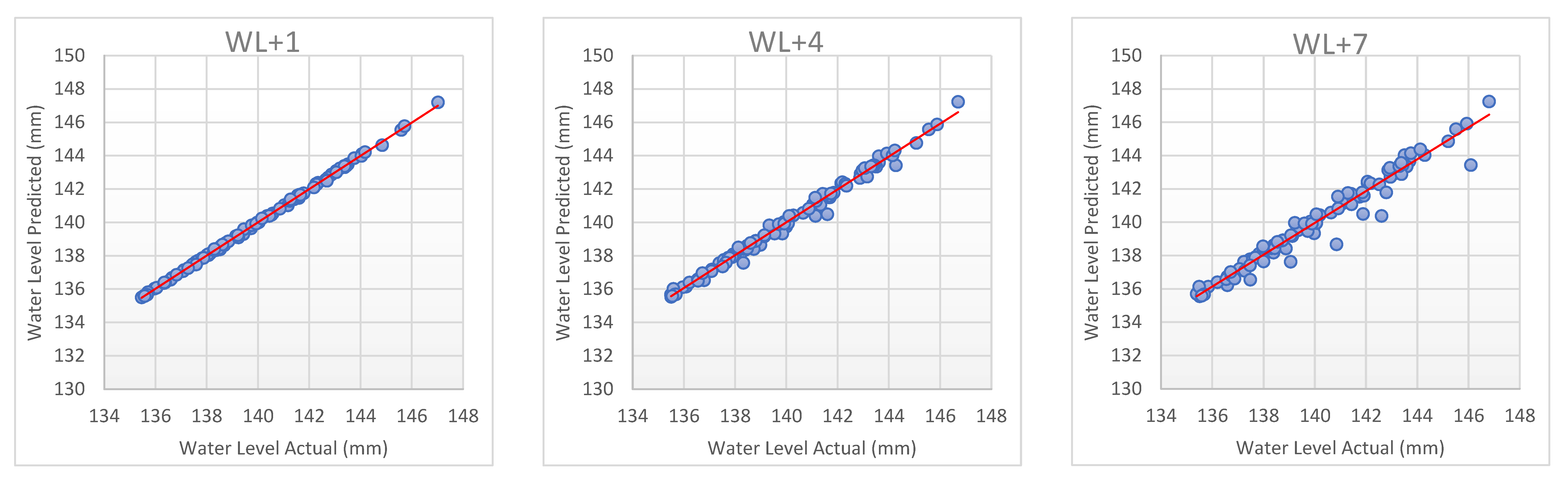
Figure 8 and Figure 9 represent scatter plot the best models of dataset. WL+1 for both scenarios of the dataset shows that the plot/distribution is close to each other compared to the next day of water level until WL+7. The scatter plot of each model for the time horizon are given in Appendix C and Appendix D. It can be seen clearly in scenario one that BLR has outstanding performance in predicting the water level in the reservoir with a high level of precision for one day and seven days ahead. Similarly, the same performance has been noticed for scenario two when BDTR was used. These results indicate that these two models can be used to predict the expected changes in water level one week ahead.

3.3. Uncertainty Analysis of Best Model of SC1 and SC2

UA of the best model for SC1 is BLR while SC2 is BDTR was calculated using 95PPU and d-factor.

Table 5. Uncertainty analysis of BLR model for SC1 and BDTR model for SC2.

Days	Statistic	BLR for SC1	BDTR for SC2
WL+1	L95PPU	0.909708687	92.4371394
	U95PPU	0.954164831	96.1198655
	d-factor	0.000075605	0.000028308
WL+2	L95PPU	0.909524827	92.301457
	U95PPU	0.954078332	96.0992443
	d-factor	0.000075771	0.000029241
WL+3	L95PPU	0.909376505	92.1516587
	U95PPU	0.953682446	95.9710899
	d-factor	0.000075350	0.000029441
WL+4	L95PPU	0.909255629	91.7296073
	U95PPU	0.953625071	95.7751477
	d-factor	0.000075458	0.00003123
WL+5	L95PPU	0.909175731	91.6601331
	U95PPU	0.953904084	95.7378567
	d-factor	0.000076068	0.000031504
WL+6	L95PPU	0.909081900	91.6177377
	U95PPU	0.953521575	95.6896427
	d-factor	0.000075577	0.000031501
WL+7	L95PPU	0.908999518	91.5594281
	U95PPU	0.953486824	95.667071
	d-factor	0.000075658	0.000031828

represent the uncertainty analysis results for seven days and one day ahead of forecasting water level.

Table 5 specifies that about 95.42%, 95.41%, 95.37%, 95.36%, 95.39%, 95.35%, and 95.35% of data for the best BLR in SC1 and 96.12%, 96.1%, 95.97%, 95.78%, 95.74%, 95.69%, 95.67% of data for the best BDTR in SC2 relate to WL+1, WL+2, WL+3, WL+4, WL+5, WL+6, and WL+7, respectively. Hence, the d-factor has values of 0.000075605, 0.000075771, 0.000075350, 0.000075458, 0.000076068, 0.000075577, 0.000075658 in SC1 and 0.000028308, 0.000029241, 0.000029441, 0.00003123, 0.000031504, 0.000031501, 0.000031828 in SC2 for WL+1, WL+2, WL+3, WL+4, WL+5, WL+6, and WL+7, respectively.

This finding of the uncertainty analysis revealed that the proposed model exhibited a high level of accuracy in predicting the water level where all 95PPU for the different time horizons attained more than 80% and the d-factor value was at a very acceptable level, which fell below this. However, in spite of such results, there is still a need for further analysis to adopt this model on another study area, which can be achieved by modifying the architecture of the proposed model since each study area has its own pattern in water level.

3.4. Taylor Diagram for Best Performance in Each Scenarios

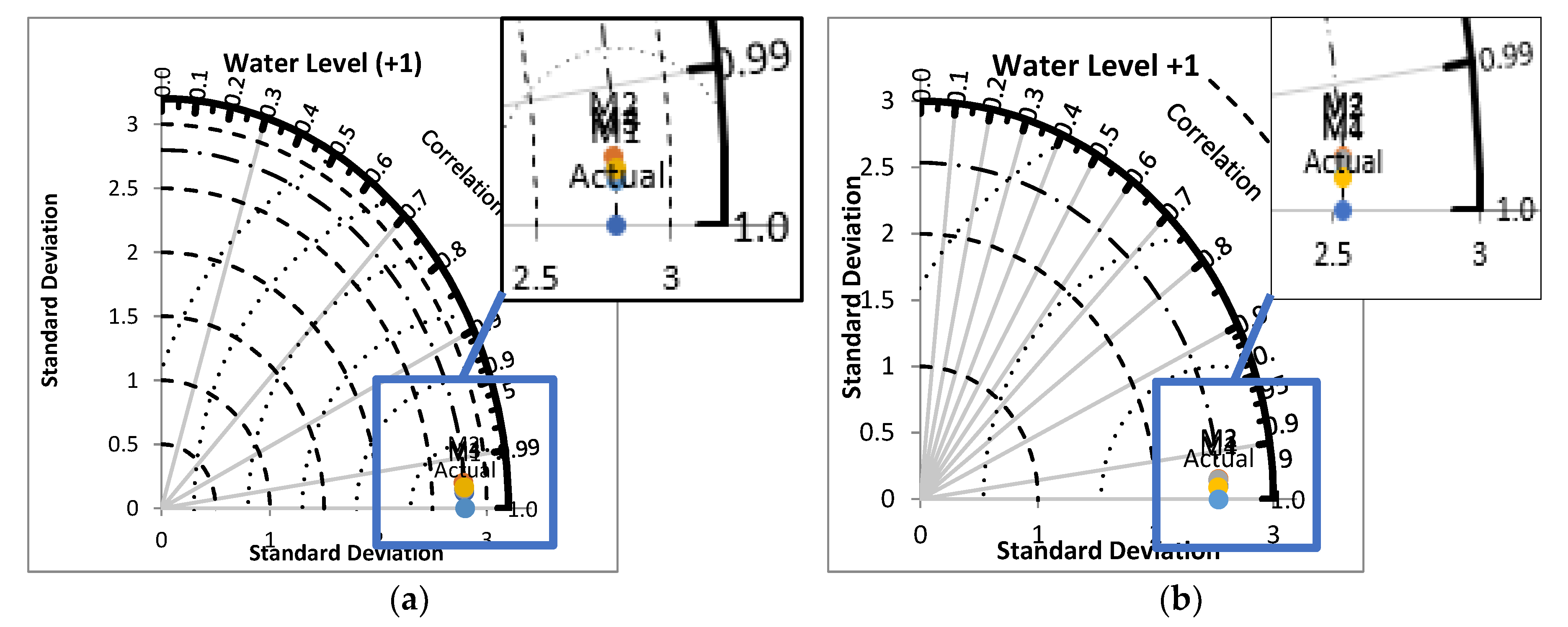
Figure 10 shows the Taylor diagram from water level one day ahead. Taylor diagrams will facilitate the comparative assessment of different models. It is used to quantify the degree of correspondence between the modeled and observed behavior in terms of three statistics: The Pearson correlation coefficient, the root-mean-square error (RMSE) error, and the standard deviation. Figure 10a shows the four models used; namely, M1 presents BLR, M2 presents NNR, M3 presents BDTR, and M4 presents DFR. Meanwhile, Figure 10b shows the four models used; namely, M1 presents DFR, M2 presents NNR, M3 presents BLR, and M4 presents BDTR. From the diagram, we can conclude that the most correspondence predicted to actual data is M1 for both scenarios, which represents BLR in SC1 and BDTR in SC2 as the closest to the actual value.

In can be seen based on the correlation and standard deviation between the actual water level and the predicted one from the proposed model that the developed model is not only capable of predicting the changes in water level accurately during the entire dataset, but also the standard deviation of predicted data is close to the actual one. This indicates that the proposed model is capable of mimicking the variation in the dataset.

3.5. Accuracy Improvement

In order to compare between scenario one and scenario two, the percentage of accuracy improvement formula was used as follow:

$$AI\%=\left(\frac{{R^2}_{\mathrm{SC}1}-{R^2}_{\mathrm{SC}2}}{{R^2}_{\mathrm{SC}1}}\right)\times 100$$

(11)

where R²_SC1 is the value of the coefficient of determination given by SC1, while R²_SC2 is the same coefficient of determination given by the proposed SC2. This comparison of R² from the best model of BDTR for the both scenario. Referring to

Table 6. Accuracy improvement with machine learning algorithms, BDTR.

Days	AI (%)
WL+1	0.1
WL+2	0.5
WL+3	0.8
WL+4	1.0
WL+5	1.7
WL+6	2.6
WL+7	3.5

, this shows that SC2 has the best result rather than SC1 since the accuracy improvement is positive. The result is the accuracy improvement getting better among the water level for the next seven days. In can be concluded that by introducing scenario two, there is noticeable improvement in predicting the changing in the water level of the reservoir. In addition to that, the accuracy improvement percentage after introducing scenario two shows that the model performs better in predicting water level in different lead times where the highest percentage of accuracy improvement is achieved when the model is used to predict the water level one week ahead.

4. Conclusions

This study investigated different Machine Learning techniques such as Boosted Decision Tree Regression (BDTR), Decision Forest Regression (DFR), Neural Network Regression (NNR), and Bayesian Linear Regression (BLR) to identify the most accurate model for water level prediction based on daily measured historical data from 1985 to 2019. Different time horizons were examined from one day ahead to seven days ahead. The results showed that all the models performed well and can mimic the actual values, however, the BLR model outperformed all other models for SC1 where the predicted values were found to be close to the coefficient of determination of 1 for forecasting water level. Meanwhile, BDTR outperformed all other models for SC2. The best model performance of R² for SC1 is 0.994992, 0.9917, 0.990856, 0.984186, 0.97562, 0.967717 while for SC2 is 0.999368, 0.997656, 0.995418, 0.993893, 0.99146, 0.990325, and 0.988958 for each water level, respectively. After conducting uncertainty for the proposed models, using 95PPU and d-factor analysis, it can be concluded that the BLR (for SC1) and BDTR (for SC2) show high satisfaction in degree of uncertainty. In this study, in spite of introducing few inputs to the proposed models, two input parameters (water level and rainfall) used in SC1 and three input parameters (water level, rainfall, and sent out) used in SC2, it can be seen that the models performed well in predicting the changes in water level with a high level of accuracy. The proposed models can be used as a tool in operating the reservoirs in Malaysia efficiently and could be an effective method for water decision makers by relying on the highly demanding new technologies such as Artificial Intelligence. However, further study is needed by including more input parameters such as the change in rainfall due to climate changes in order to improve the accuracy of the model and also investigate the impact of the projected rainfall on the water level of the reservoir.

References

1. Hu Hussain, W.; Ishak, W.; Ku-mahamud, K.R.; Norwawi, N. Neural network application in reservoir water level forecasting and release decision. Int. J. New Comput. Archit. Appl. 2011, 1, 265–274. [Google Scholar]
2. Ashaary, N.A.; Ishak, W.H.W.; Ku-mahamud, K.R. Forecasting the change of reservoir water level stage using neural network. In Proceedings of the 5th International Conference on Computing and informatics, ICOCI 2015, Istanbul, Turkey, 11–13 August 2015; pp. 692–697. [Google Scholar]
3. Zaji, A.H.; Bonakdari, H.; Gharabaghi, B. Reservoir water level forecasting using group method of data handling. Acta Geophys. 2018, 66, 717–730. [Google Scholar] [CrossRef]
4. Mullainathan, S.; Spiess, J. Machine learning: An applied econometric approach. J. Econ. Perspect. 2017, 31, 87–106. [Google Scholar] [CrossRef] [Green Version]
5. Alpaydin, E. Machine Learning: The New AI; Essential Knowledge series; MIT Press: Cambridge, MA, USA, 2016. [Google Scholar]
6. Alpaydin, E. Introduction to Machine Learning; MIT Press: Cambridge, MA, USA, 2014. [Google Scholar]
7. AlDahoul, N.; Htike, Z. Utilizing hierarchical extreme learning machine based reinforcement learning for object sorting. Int. J. Adv. Appl. Sci. 2019, 6, 106–113. [Google Scholar] [CrossRef]
8. Hu, W.; Singh, R.R.P.; Scalettar, R.T. Discovering phases, phase transitions, and crossovers through unsupervised machine learning: A critical examination. Phys. Rev. E 2017, 95, 1–14. [Google Scholar] [CrossRef] [Green Version]
9. Wang, L. Discovering phase transitions with unsupervised learning. Phys. Rev. B 2016, 94, 2–6. [Google Scholar] [CrossRef] [Green Version]
10. Ahmed, A.N.; Othman, F.B.; Afan, H.A.; Ibrahim, R.K.; Fai, C.M.; Hossain, M.S.; Ehteram, M.; Elshafie, A. Machine learning methods for better water quality prediction. J. Hydrol. 2019, 578, 124084. [Google Scholar] [CrossRef]
11. Mohammed, M.; Khan, M.B.; Bashier, E.B.M. Machine Learning: Algorithms and Applications; CRC Press: Boca Raton, FL, USA, 2017; Volume 91. [Google Scholar]
12. Tokar, A.S.; Markus, M. Precipitation-runoff modelling using artificial neural networks and conceptual models. J. Hydrol. Eng. 2000, 5, 156–161. [Google Scholar] [CrossRef]
13. Karunanithi, N.; Grenney, W.J.; Whitley, D.; Bovee, K. Neural networks for river flow prediction. J. Comput. Civ. Eng. 1994, 8, 201–220. [Google Scholar] [CrossRef]
14. Terzi, Ö.; Ergin, G. Forecasting of monthly river flow with autoregressive modeling and data-driven techniques. Neural Comput. Appl. 2013, 25, 179–188. [Google Scholar] [CrossRef]
15. Yaseen, Z.M.; El-shafie, A.; Jaafar, O.; Afan, H.A.; Sayl, K.N. Artificial intelligence based models for stream-flow forecasting: 2000–2015. J. Hydrol. 2015, 530, 829–844. [Google Scholar] [CrossRef]
16. Najah, A.A.; El-Shafie, A.; Karim, O.A.; Jaafar, O. Integrated versus isolated scenario for prediction dissolved oxygen at progression of water quality monitoring stations. Hydrol. Earth Syst. Sci. Discuss. 2011, 8, 6069–6112. [Google Scholar] [CrossRef]
17. Hipni, A.; El-shafie, A.; Najah, A.; Karim, O.A.; Hussain, A.; Mukhlisin, M. Daily forecasting of dam water levels: Comparing a Support Vector Machine (SVM) Model with Adaptive Neuro Fuzzy Inference System (ANFIS). Water Resour. Manag. 2013, 27, 3803–3823. [Google Scholar] [CrossRef]
18. Piri, J.; Kahkha, M.R.R. Prediction of water level fluctuations of chahnimeh reservoirs in Zabol using ANN, ANFIS and Cuckoo optimization algorithm. Iran. J. Health Saf. Environ. 2016, 4, 706–715. [Google Scholar]
19. Zhang, S.; Lu, L.; Yu, J.; Zhou, H. Short term water level prediction using different artificial intelligent models. In Proceedings of the 5th International Conference on Agro-geoinformatics (Agro-geoinformatics), Tianjin, China, 18–20 July 2016. [Google Scholar]
20. Üneş, F.; Demirci, M.; Taşar, B.; Kaya, Y.Z.; Varçin, H. Estimating dam reservoir level fluctuations using data-driven techniques. Pol. J. Environ. Stud. 2018, 28, 3451–3462. [Google Scholar] [CrossRef]
21. Soleymani, S.A.; Goudarzi, S.; Anisi, M.H.; Hassan, W.H.; Idris, M.Y.I.; Shamshirband, S.; Noor, N.M.; Ahmedy, I. A novel method to water level prediction using RBF and FFA. Water Resour. Manag. 2016, 30, 3265–3283. [Google Scholar] [CrossRef]
22. Seo, Y.; Kim, S.; Kisi, O.; Singh, V.P. Daily water level forecasting using wavelet decomposition and artificial intelligence techniques. J. Hydrol. 2014, 520, 224–243. [Google Scholar] [CrossRef]
23. Guo, T.; He, W.; Jiang, Z.; Chu, X.; Malekian, R.; Li, Z. An improved LSSVM model for intelligent prediction of the daily water level. Energies 2018, 12, 112. [Google Scholar] [CrossRef] [Green Version]
24. Damian, D.C. A critical review on artificial intelligence models in hydrological forecasting how reliable are artificial intelligence models. Int. J. Eng. Tech. Res. 2019, 8, 365–378. [Google Scholar]
25. Kohavi, R. A study of cross-validation and bootstrap for accuracy estimation and model selection. In Proceedings of the 14th International Joint Conference on Artificial Intelligence, Montreal, QC, Canada, 20–25 August 1995. [Google Scholar]
26. Devijver, P.A.; Kittler, J. Pattern Recognition: A Statistical Approach; Prentice Hall: Upper Saddle River, NJ, USA, 1982. [Google Scholar] [CrossRef]
27. Liu, H.; Cocea, M. Semi-random partitioning of data into training and test sets in granular computing context. Granul. Comput. 2017, 2, 357–386. [Google Scholar] [CrossRef] [Green Version]
28. Muslim, T.O.; Ahmed, A.N.; Malek, M.A.; Afan, H.A.; Ibrahim, R.K.; El-shafie, A.; Sapitang, M.; Sherif, M.; Sefelnasr, A.; El-shafie, A. Investigating the influence of meteorological parameters on the accuracy of sea-level prediction models in Sabah, Malaysia. Sustainability 2020, 12, 1193. [Google Scholar] [CrossRef] [Green Version]
29. Boosted Decision Tree Regression. Azure Machine Learning Studio. Microsoft Docs. Available online: https://docs.microsoft.com/en-us/azure/machine-learning/studio-,odule-reference/boosted-decision-tree-regression (accessed on 9 December 2019).
30. Boosted Trees Regression. Turi Machine Learning Platform User Guide. Available online: https://turi.com/learn/userguide/supervised-learning/boosted_trees_regression.html (accessed on 9 December 2019).
31. Pros and cons of classical supervised ML algorithms. rmartinshort. Available online: https://rmartinshort.jimdofree.com/2019/02/24/pros-and-cons-of-classical-supervised-ml-algorithms/ (accessed on 9 December 2019).
32. Jumin, E.; Zaini, N.; Ahmed, A.N.; Abdullah, S.; Ismail, M.; Sherif, M.; Sefelnasr, A.; El-shafie, A. Machine learning versus linear regression modelling approach for accurate ozone concentrations prediction. In Engineering Applications of Computational Fluid Mechanics; Springer: Berlin/Heidelberg, Germany, 2020; Volume 14, pp. 713–725. [Google Scholar]
33. Criminisi, A. Decision Forests: A unified framework for classification, regression, density estimation, manifold learning and semi-supervised learning. Found. Trends Comput. Graph. Vis. 2011, 7, 81–227. [Google Scholar] [CrossRef]
34. Tan, L.K.; McLaughlin, R.A.; Lim, E.; Aziz, Y.F.A.; Liew, Y.M. Fully automated segmentation of the left ventricle in cine cardiac MRI using neural network regression. J. Magn. Reson. Imaging 2017, 48, 140–152. [Google Scholar] [CrossRef] [PubMed]
35. Catal, C.; Ece, K.; Arslan, B.; Akbulut, A. Benchmarking of regression algorithms and time series analysis techniques for sales forecasting. Balk. J. Electr. Comput. Eng. 2019, 7, 20–26. [Google Scholar] [CrossRef] [Green Version]
36. Hyndman, R.J.; Koehler, A.B. Another look at measures of forecast accuracy. Int. J. Forecast. 2006, 22, 679–688. [Google Scholar] [CrossRef] [Green Version]
37. Miller, T.B.; Kane, M. The precision of change scores under absolute and relative interpretations. Appl. Meas. Educ. 2001, 14, 307–327. [Google Scholar] [CrossRef]
38. Nagelkerke, N.J.D. A note on a general definition of the coefficient of determination. Biometrika 1991, 78, 691–692. [Google Scholar] [CrossRef]
39. Cheng, C.T.; Feng, Z.K.; Niu, W.J.; Liao, S.L. Heuristic methods for reservoir monthly inflow forecasting: A case study of Xinfengjiang Reservoir in Pearl River, China. Water 2015, 7, 4477–4495. [Google Scholar] [CrossRef]
40. Kamiński, B.; Jakubczyk, M.; Szufel, P. A framework for sensitivity analysis of decision trees. Cent. Eur. J. Oper. Res. 2018, 26, 135–159. [Google Scholar] [CrossRef]
41. Abbaspour, K.C.; Yang, J.; Maximov, I.; Siber, R.; Bogner, K.; Mieleitner, J.; Zobrist, J.; Srinivasan, R. Modelling hydrology and water quality in the pre-alpine/alpine thur watershed using SWAT. J. Hydrol. 2007, 333, 413–430. [Google Scholar] [CrossRef]
42. Noori, R.; Hoshyaripour, G.; Ashrafi, K.; Araabi, B.N. Uncertainty analysis of developed ANN and ANFIS models in prediction of carbon monoxide daily concentration. Atmos. Environ. 2010, 44, 476–482. [Google Scholar] [CrossRef]
43. Noori, R.; Yeh, H.-D.; Abbasi, M.; Kachoosangi, F.T.; Moazami, S. Uncertainty analysis of support vector machine for online prediction of five-day biochemical oxygen demand. J. Hydrol. 2015, 527, 833–843. [Google Scholar] [CrossRef]
Figure 1. Location of Kenyir Dam.
Sustainability 12 06121 g001
Figure 2. Station layout of Kenyir Dam.
Sustainability 12 06121 g002
Figure 3. Boosted decision tree regression.
Sustainability 12 06121 g003
Figure 4. Decision forest regression.
Sustainability 12 06121 g004
Figure 5. Neural network regression.
Sustainability 12 06121 g005
Figure 6. Bayesian linear regression.
Sustainability 12 06121 g006
Figure 7. Methodology flow chart using machine learning algorithms to forecast values.
Sustainability 12 06121 g007
Figure 8. Scatter plot of water level actual versus water level forecasted for the best models (Bayesian Linear Regression (BLR)) for SC1.
Sustainability 12 06121 g008
Figure 9. Scatter plot of water level actual versus water level forecasted for the best models (BDTR) for SC2.
Sustainability 12 06121 g009
Figure 10. Taylor diagram of water level one day ahead; (a) SC1 and (b) SC2.
Sustainability 12 06121 g010