Article

A Successful Approach of the First Ecological Compensation Demonstration for Crossing Provinces of Downstream and Upstream in China

1
Environmental Criteria, Ministry of Education, and Tianjin Key Laboratory of Environmental Remediation and Pollution Control, College of Environmental Science and Engineering, Nankai University, Tianjin 300071, China
2
State Environmental Protection Key Laboratory of Environmental Planning and Policy Simulation, Chinese Academy for Environmental Planning, Beijing 100012, China
3
Ministry of Transport of the People’s Republic of China, Tianjin Research Institute for Water Transport Engineering, Tianjin 300456, China
*
Author to whom correspondence should be addressed.
Sustainability 2020, 12(15), 6021; https://doi.org/10.3390/su12156021
Submission received: 10 June 2020 / Revised: 17 July 2020 / Accepted: 24 July 2020 / Published: 27 July 2020

Abstract

:
As the first pilot provincial water environmental compensation set up at the national level, the Xin’anjiang River Basin plays a very important exemplary and guiding role in the ecological compensation of transboundary basins in China. There is no paper evaluating the environmental performance in watershed scale after getting rid of the natural factor’s effect. Here we issue a new approach to evaluate it, combing the SPAtially Referenced Regression On Watershed attributes (SPARROW) models and data envelopment analysis (DEA) method, based on counterfactual scenarios. After ecological compensation, the results show that the decrease of total nitrogen (TN) non-point source export coefficient was stable (17.16–17.78% in different sources), while that of total phosphorus (TP; 8.51–17.75%) and permanganate index (CODMn; 13.10–21.41%) was not. The projects of fertilizer application’s effects were relatively obvious; on average, the decreases of the export coefficients were 17.16%, 17.75%, and 21.41% in TN, TP, and CODMn models, respectively, showing the importance of eco-compensation regulation, not only in non-point source pollution reduction but also resulting in high levels of eco-compensation efficiencies, especially in scale efficiencies. By assessing parameter and modeling uncertainty with the use of the generalized likelihood uncertainty estimation (GLUE) method, the models’ structure well represents the hydrological behavior. This study also provides policymakers with a new perspective in accurately measuring the impact of environmental performance, to guide the next step of environmental investment optimization.

1. Introduction

High-quality development will replace fast growth as a fundamental economic development target for China [1]. China was gradually entering the new normal of economic growth [2,3,4], under which the economic structure would be optimized and effects would far exceed those environmental regulations and policies [5]. After decades of rapid economic development, water quality problems have become constraints for green development in China [6]. To address devastating water environmental crises and to improve the quality of economic developments, China has already implemented multiple regional and national policies [7,8,9]. It is important to find suitable environmental water management methods to adapt to China’s economic conditions and the administrative system. China’s existing water management system is managed in accordance with administrative regions instead of river basins [10]. Ecological compensation is an important type of design and institutional arrangements coordinate regional development and ecological environment [11,12]. Ecological compensation in China has improved with the progress of environmental protection [13,14], making the definition close to the new concept of Payment for Ecosystem Services (PES) [15]. However, the practice of river basin ecological compensation in China mostly exists within the jurisdiction of one province, and the practice across provinces with more complicated relations is rare.
After eight years of preparations, in 2012 the Ministry of Finance and the Ministry of Environmental Protection (renamed Ministry of Ecological Environment in 2018) in China formally launched the first demonstration project to address upstream-downstream ecological compensation across provinces in Xin’anjiang River Basin (XRB), which is of great guiding significance for China [
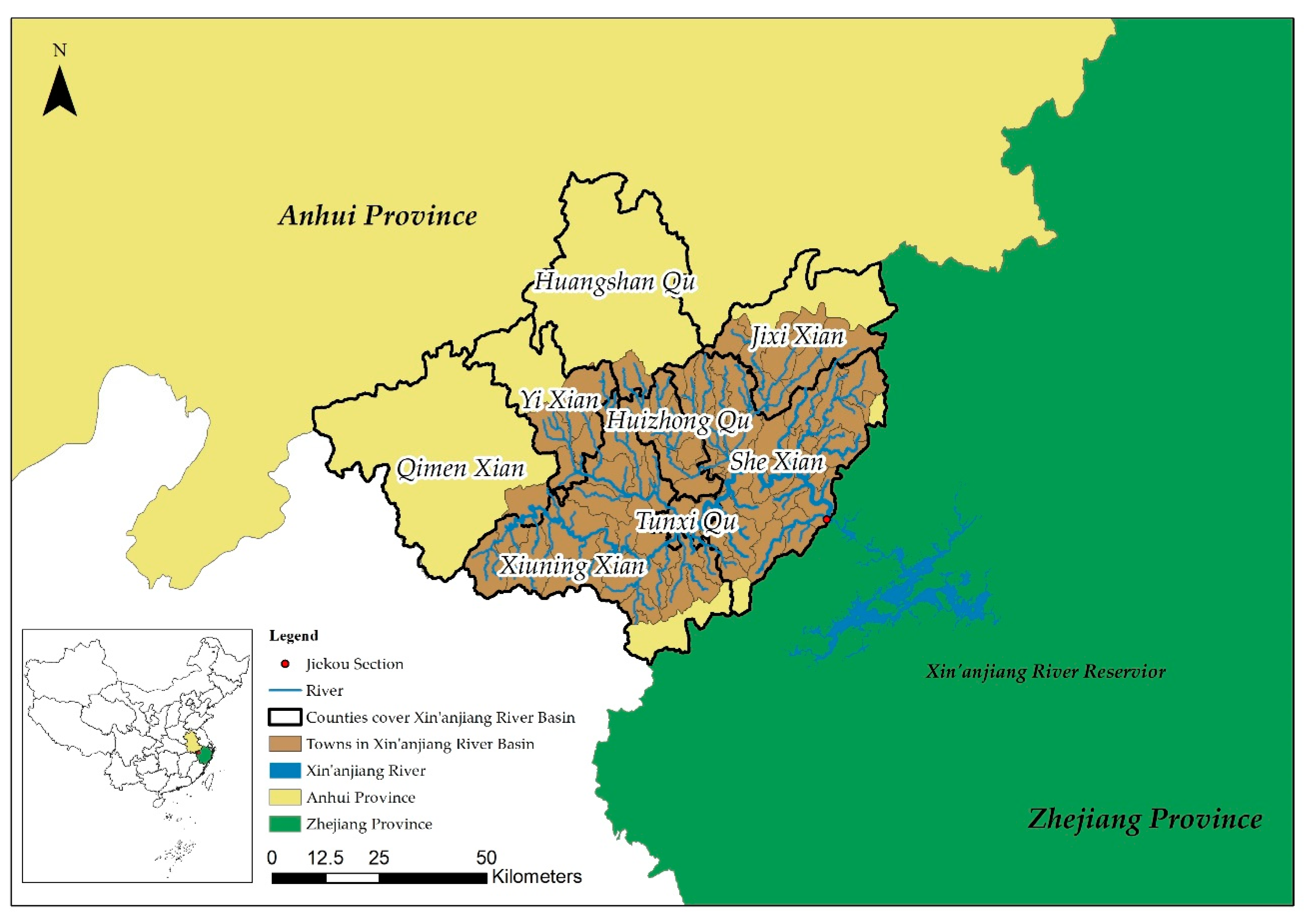
16]. XRB, located at the junction of Zhejiang province and Anhui province (Figure 1), is the largest inflow river of the Qiantangjiang River system and Qiandao Lake in Zhejiang province. XRB and Qiandao Lake are not only important drinking water sources of Zhejiang and Anhui provinces [17] but also ecological security barriers of the Yangtze River Delta region [16].
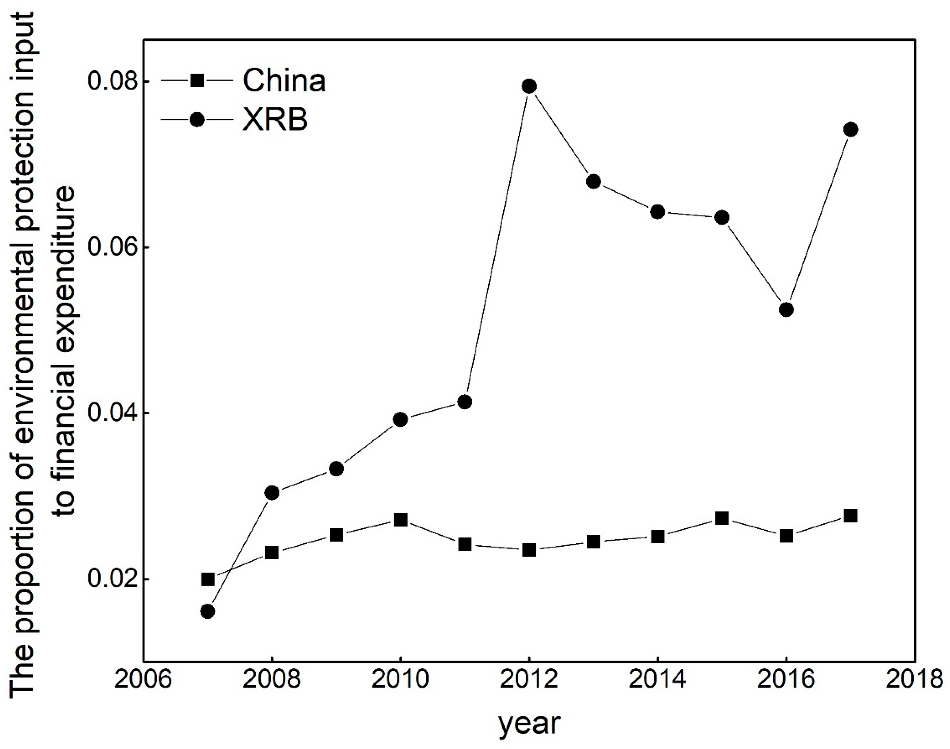
Environmental protection has always been taken seriously in the XRB. The proportions of environmental protection input to financial expenditure in China and XRB are listed in Figure 2 since 2007 [18], which was the year that environmental protection spending began to take into fiscal spending in China. Data are collected from the Ministry of Finance of China and the Bureau of Finance in Huangshan City and Jixi County, which contain the XRB. Although in 2007, the proportions in XRB were greater than those in China. The financial expenditure had significant differences (p < 0.05) before and after 2012, which was the year that ecological compensation began. Thus, we take the period of 2012–2017 as consideration of ecological compensation effects.
This project was divided into two stages from 2012 to 2017: first-round stage (2012–2014, XAJ1) and second-round stage (2015–2017, XAJ2), with the total spending of 146.32 hundred million Yuan (Figure S1). With a guaranteed system, diversified funds, and reasonable basis of compensation (see Supplementary Information for details), the mode in XRB was successfully demonstrated, guaranteeing the water quality of downstream. A sufficient preliminary investigation was made to determine the main direction of compensation funds. Each stage summarizes the achievements of each stage. The system ensures that the compensation funds are specifically used for the industrial structure adjustment and industrial layout optimization of the XRB, comprehensive river basin management, water environment protection, water pollution control, and ecological protection. The corresponding projects (Table 1) include sewage treatment, garbage disposal, pesticide and chemical fertilizer treatment, livestock and poultry management, and comprehensive measures.
Identifying precisely how much environmental improvement was due to the compensation funds and whether the funds had been effectively used in different counties is important to evaluate the ecological compensation policy, and is crucial information for decision-makers, particularly in the new normal of China’s economy. We chose XRB as our study area not only because the standard of compensation is based on its water quality, but also because the compensation funds were all used to improve the water quality in the period of 2012–2017, which is typical for calculating the environmental performance. The environmental effects were evaluated through a historical trend (2007–2011) analysis of water quality loads to estimate the counterfactual (without ecological compensation) loads in the period of ecological compensation (2012–2017). Yet so far existing studies have focused on the standard mechanism of the ecological compensation [14,19]. Other research has examined the efficiency of payment of ecosystem services [20,21,22]. However, there are no adequate analyses of the river basin ecological compensation performances with getting rid of the natural conditions’ influences.
This article aims to bridge this gap by innovatively using data envelopment analysis (DEA), which uses different kinds of environmental investments as input and counterfactual SPAtially Referenced Regression On Watershed attributes (SPARROW) model results in the watershed as output, to evaluate the environmental investments’ efficiency in different counties in the XRB. This approach should be generalizable to different areas and thus valuable beyond the immediate application. The next sections provide (1) a brief introduction of the data sources, the DEA method and SPARROW model and their applications in models, (2) a detailed analysis of each result, and (3) a discussion about the references of the successful approach of the first ecological compensation demonstration for crossing provinces of downstream and upstream in China. To our knowledge, this is the first use of counterfactual scenarios to estimate the environmental performances and related efficiencies in the valuation of ecological compensation. Influences of social and political impacts are beyond the scope of this piece of work due to the lack of data and related researches.

2. Materials and Methods

2.1. Data Sources

Precipitation data were provided in 48 precipitation data sites in the XRB. Water quality data were collected monthly at 60 sites. Flux data used to calibrate the curve numbers were provided by the Environmental Protection Bureau of Huangshan City and Jixi County. Fertilizers and pesticide data were both taken from Anhui statistic yearbook (2007–2017) and provided by XRB Environmental Protection Bureau. The population data were obtained from the government statistical agency website.

2.2. SPARROW Models

The SPARROW water-quality model is a nonlinear least-squares multiple regression model to estimate pollutant sources and tracks the sources of the contaminants [23,24]. This model has been already used successfully in the XRB [17]. To better illustrate the effect of ecological compensation, we chose different sources and water-soil variables to adapt the ecological compensation projects. The SPARROW model easily calculates the delivery loads to the target section (Jiekou Section is the target section we considered in this case, which is also the joint of Anhui province and Zhejiang province, see Figure 1), which makes it quite suitable for Chinese water quality management [25]. The models are based on a detailed stream reach network with 304 sub-catchments delineated from 30-km digital elevation models (DEMs), using ArcHydro [26] extension in ArcGIS. Mean annual water yields were calculated using the Soil Conservation Service (SCS) curve number (CN) method [27].
The structures of SPARROW models are limited to the quantity of the water quality monitor sites [
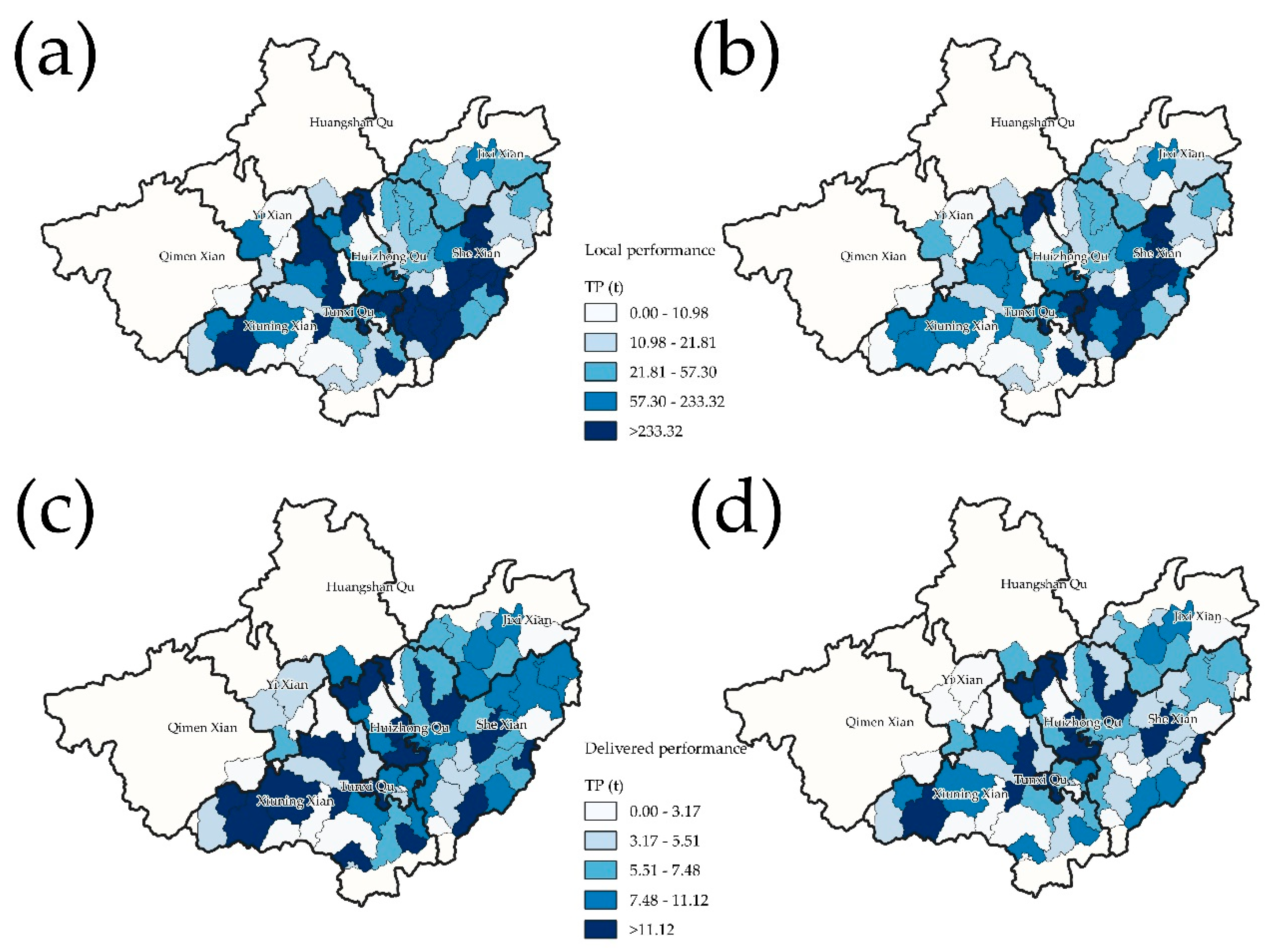
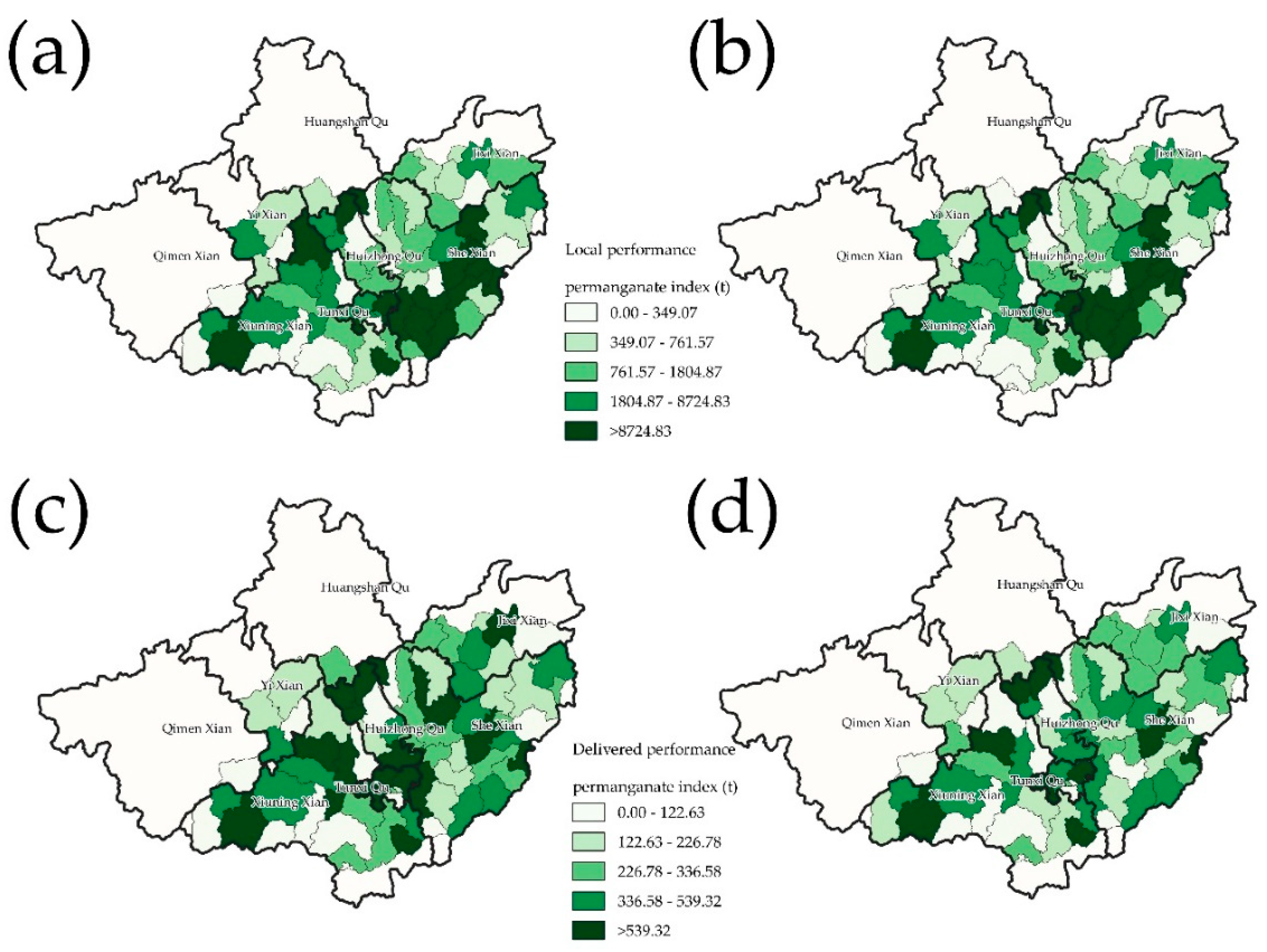
28]. After testing several SPARROW models’ structures, we simulated the mean annual flux of total nitrogen (TN), total phosphorus (TP), and permanganate index (CODMn) in streams as functions of four sources, three climatic and landscape factors that influence pollutant delivery to streams, and pollutant removal in streams (there is no reservoir in this case). Pollutant sources contain industrial point sources, agricultural plantation sources, livestock and poultry raising sources, and domestic pollution sources. Industrial point sources are the sources of industrial wastewater discharge. Agricultural plantation sources include commercial fertilizer in TN and TP models while including pesticides in CODMn models. Additionally, we dealt with the population data as the same methods as in the previous study [17] to represent domestic pollution sources.
Measurements of nutrient water quality at stream monitoring sites collected during 2007–2017 were used to develop observations of mean annual nitrogen load as the response variable in the SPARROW regression equations. The mean annual load was estimated as the product of daily streamflow and estimated daily concentration, which was modeled from nutrient water-quality data and streamflow data. We calculated the flux as the same method of the previous study [17].
According to the best model results, the model estimates pollutant delivery to streams, including slope, temperature, precipitation in TN models, and CODMn models. In TP models, the pollutant delivery parameters are slope, drainage density, and precipitation.

2.3. Counterfactual Scenarios Accounting

The year 2012 is a time node of great significance (Figure 2); the counterfactual scenario assumes no eco-compensation happened. In this scenario, the mean results of 2007–2011 would be used in the coefficient of industrial point sources. All the coefficients of non-point sources, including agricultural plantations sources, livestock and poultry raising sources, and domestic pollution sources, would be influenced greatly by the precipitation. Thus, the improved export coefficient model (IECM) [29] is used to calculate the export coefficients under the situation of the period 2012–2017 if no eco-compensation happened. The IECM is expressed as:
L = i = 1 n α β E i [ A i ( I i ) ] + p
where L is loss of nutrients (kg); Ei is the export coefficient for nutrient source i (kg/ca·yr or kg/km2·yr); Ai is area of the catchment occupied by land use type i (km2), or number of livestock type i, or of people; Ii is the input of nutrients to source i (kg); p is the input of nutrients from precipitation (kg); α is the precipitation impact factor; β is the terrain impact factor.
The differences between the actual and counterfactual TN, TP, and CODMn loads would be considered as environmental performances, which removed the influences of precipitation.

2.4. DEA Method

DEA is a technique to measure efficiency that uses a set of comparable decision-making units (DMUs), calculating the efficient frontier and identify benchmarks [30]. Limited by the lack of data and related research, here we only used the basic input-oriented DEA model, which is used to measure environmental investments’ efficiency.
We chose the inflation-adjusted ecological compensation funds as input, and environmental performances as output to calculate technique efficiencies, pure technique efficiencies, and scale efficiencies in different towns to get more DMUs, fitting the model well. Additionally, we used the mean value of the results in different counties, which was the smallest unit that accepted the funds in this case.

2.5. Generalized Likelihood Uncertainty Estimation (GLUE) Method

The GLUE method is extensively used in global sensitivity and uncertainty analysis [31,32,33,34,35], due to the simplicity and applicability to nonlinear systems [31]. Compared to other methods, GLUE is easy to implement. By sampling the prior parameter space using an adaptive Markov Chain Monte Carlo (MCMC) scheme, the computational efficiency of GLUE is improved [36,37]. We used GLUE method in this study to make Monte Carlo sampling from a feasible parameter space with uniform distribution, calculating the likelihood values of behavioral parameter sets. The Nash–Sutcliffe efficiency (ME) was chosen as the likelihood function.
ME = 1   ( Q o b s Q s i m )   ( Q o b s Q ¯ o b s ) = 1 σ i 2 σ o b s 2
where Q ¯ o b s represents mean values of observed streamflows; σ i 2 is the error variance for the ith model; σ o b s 2 is the variance of observations.

3. Results

3.1. Estimations of SPARROW Models Parameters

Table 2, Table 3 and Table 4 display the values of parameters in SPARROW TN models, TP models, and CODMn models. The parameters of industrial point sources represent the proportion of loads delivered to the river; the ranges of coefficients in TN models, TP models, and CODMn models are 0.871–1.122, 0.741–1.257, and 0.405–0.623, respectively. The reason that some parameters of industrial point sources are greater than 1 may be caused by the uncertainty of the original data.
The parameters in agricultural plantation sources of TN and TP models represent the fertilizer loss coefficient, while the parameters represent the pesticide loss coefficient in the CODMn models. The ranges of agricultural plantation sources’ coefficients in TN models, TP models, and CODMn models are 0.164–0.266, 0.009–0.016, and 0.166–0.299, respectively, within the range of estimates obtained in the previous study [38].
The parameters in livestock and poultry raising sources represent the pollutants producing coefficients of the pig equivalent in the models. The ranges of livestock and poultry raising sources’ coefficients in TN models, TP models, and CODMn models are 3.373–5.516 kg/yr·capita, 0.495–0.847 kg/yr·capita, and 7.300–13.159 kg/yr·capita, respectively, within the range of estimates obtained in the previous study [38].
The parameters in domestic pollution sources represent the pollutants producing coefficients of the population in the models. The ranges of domestic pollution sources’ coefficients in TN models, TP models, and CODMn models are 1.445–2.775 kg/yr·capita, 0.013–0.023 kg/yr·capita, and 5.849–8.482 kg/yr·capita, respectively, within the range of estimates obtained in the previous study [38].
Tables S1–S3 display the p-values of SPARROW models parameters estimation. There are 99 parameters in each group of SPARROW models. There are 87, 92, and 94 parameter estimations that lie in the 99% confidence interval in SPARROW TN models, TP models, and CODMn models, respectively.
Pollution source apportionment can help in identifying non-point sources as the main pollution sources in XRB. The average source shares of TN loads (industrial point sources/agricultural plantations sources/livestock and poultry raising sources/domestic pollution sources = 1.59/35.90/46.01/16.51) indicated that livestock and poultry raising sources were the predominant nitrogen source (Table 5). After ecological compensation, the proportion of industrial point sources decreased significantly. The reduction of nutrients from point sources in the XRB is important because the effect had instant results.
The source shares of TP loads (industrial point sources/agricultural plantations sources/livestock and poultry raising sources/domestic pollution sources = 0.04/2.60/95.27/2.09) also indicated that livestock and poultry raising sources contributed most (Table 6). Point sources of TP could be negligible.
The source shares of CODMn loads (industrial point sources/agricultural plantations sources/livestock and poultry raising sources/domestic pollution sources = 1.99/26.37/42.72/28.92) are listed in Table 7. After ecological compensation, the proportion of livestock and poultry raising sources decreased significantly.

3.2. Changes in Export Coefficient

We define the difference between export coefficients of non-point sources in counterfactual scenarios and realistic situations as the decrease in export coefficient after ecological compensation. The results (Figure 3) determine the perspective of environmental performances.
In general, the decrease of non-point source in XAJ2 was better than that in XAJ1, especially in the last year, environmental performance may be delayed after the implementation of the project. The decrease of TN non-point source export coefficients was stable (17.16–17.78% in different sources), while TP (8.51–17.75%) and CODMn (13.10–21.41%) were not. The projects of fertilizer application’s effects were relatively obvious; on average, the decreases of the export coefficients were 17.16%, 17.75%, and 21.41% in TN, TP, and CODMn models, respectively.

3.3. Environmental Performance Accounting

Environmental performance was calculated in two perspectives: the local performance and delivered performance. Local performance was based on the change of TN, TP, and CODMn loads generated in local between non-point sources in counterfactual scenarios and realistic situations, while the delivered performance was based on the loads delivered to the XRB’s export (Jiekou Section). Delivered yield refers to the net amount of TN, TP, and CODMn exported per area from the basin after all riverine losses were taken into account [39].
Additionally, environmental performance in XAJ1 was based on the change between XAJ1 and the period of 2007–2011 (before ecological compensation); the environmental performance in XAJ2 should be reflected by the performance strictly in XAJ2, thus it is the result of the changes between XAJ2 and the period of 2007–2011 minus the changes between XAJ1 and the period of 2007–2011.
In Figure 4, Figure 5 and Figure 6, we found that the local and delivered performance in XAJ1 was better than that in XAJ2; it was more difficult to make much improvement in the areas which had already made improvements. From 2012 to 2017, in the perspective of the net amount, the environmental performance of CODMn was the best, with the average amount of 7283.32 t and 346.95 t of local performance and delivered performance, respectively. The environmental performance of TN was the second, with the average amount of 73.40 t and 1659.66 t of local performance and delivered performance, respectively. The environmental performance of CODMn was the best, with the average amount of 7.41 t and 167.53 t of local performance and delivered performance, respectively. The local performance was focused on the main pollution area (She Xian and Tunxi Qu), while the delivered performance shows more spatial distribution.

3.4. Environmental Investment Efficiency Accounting

Table 8 shows the average efficiency of environmental investment, the efficiencies in XAJ1 were much better than that in XAJ2; the average efficiencies based on local performance were 0.270 and 0.156 in XAJ1 and XAJ2, respectively; the average efficiencies based on delivered performance were 0.547 and 0.184 in XAJ1 and XAJ2, respectively. The efficiencies based on delivered performance were much better than that in local performance.
Table 9 shows the average scale efficiency of environmental investment. The scale efficiencies in XAJ1 were better than that in XAJ2; the average scale efficiencies based on local performance were 0.926 and 0.513 in XAJ1 and XAJ2, respectively. The average scale efficiencies based on delivered performance were 0.841 and 0.544 in XAJ1 and XAJ2, respectively. The scale efficiencies based on local performance were better than that in local performance in XAJ1, while they were on the contrast in XAJ2.
Table 10 shows the average pure efficiency of environmental investment. The pure technique efficiencies in XAJ1 were better than that in XAJ2; the average pure technique efficiencies based on local performance were 0.285 and 0.244 in XAJ1 and XAJ2, respectively. The average pure technique efficiencies based on delivered performance were 0.658 and 0.362 in XAJ1 and XAJ2, respectively. The pure technique efficiencies based on delivered performance were much better than that in local performance.

3.5. Global Sensitivity and Uncertainty Analysis

The uncertainties associated with the results mainly derived from the data regarding the pollutants and the joint models’ results. As the first ecological compensation demonstration for crossing provinces of downstream and upstream in China, the data collection was supported and guaranteed by the local government. There is nonetheless some uncertainty that errors in data may affect the results.
In total, 100,000 samples were drawn, and 163,191 parameter sets with ME bigger than 0.8 were retained as behavioral sets accounting for about 16% of the total samples. By assessing parameters and modeling uncertainties of the SPARROW models with the use of the GLUE method, the paper evaluates the results of the environmental investment efficiencies. From the unimodal posterior distributions, parameter estimates can be unambiguously inferred as modal values, while the shape of the distributions indicates the degree of uncertainty of the estimates [33]. By running the model with the behavioral parameter sets, the percentage of the observation coverage of the GLUE method is 88%.
Tables S4–S6 show the sensitivity of individual parameters expressed as the deviation between the cumulative likelihood distribution curves of the posterior and prior parameters. Table 11, Table 12 and Table 13 show the summary of posterior distribution for each parameter in SPARROW models. Not all the parameters displayed significant sensitivity. SPARROW TN models are highly sensitive to the coefficient of domestic pollution sources, fertilizer application, slope, temperature and k1; SPARROW TP models are highly sensitive to the coefficient of fertilizer application, drainage density, and k1; SPARROW CODMn models are highly sensitive to the coefficient of fertilizer application, slope, and precipitation.

4. Discussion and Conclusions

Given its previous successes in XRB with the junction of Anhui province and Zhejiang province, the experience was used for reference in Jiuzhoujiang River with the junction of Guangxi autonomous region and Guangdong province basin and Hanjiang-Tingjiang River Basin with the junction of Fujian province and Guangdong province as the next two ecological compensation pilots in China. Not surprisingly, similar measures will be used in more and more river basins. The specific influences of ecological compensation demonstration in basin-scale have not been effectively quantified in China, mainly due to the lack of methods to get rid of the influence of natural factors.
This paper makes a substantial exploration of the first ecological compensation, striving to more accurately measure the impact of environmental performance. The results show that the approach of the first ecological compensation demonstration for crossing provinces of downstream and upstream in China is a successful one. The programs have produced many positive ecological outcomes. At the XAJ1, the environmental performances and efficiencies were higher than those in XAJ2. The decrease of non-point source in XAJ2 was better than that in XAJ1, due to the accumulation of the environmental effects. The environmental investments achieved the goals, and both local performance and delivered performance of different sources were great.
With systematic planning and diversified funding, the approach of the compensation was effective. This study deepens our understanding of how to accurately measure the impact of environmental performance, which will provide future researchers with references to establish models to get rid of the natural factors’ influences, providing policy makers with a new perspective in the next step of environmental investment optimization.

Supplementary Materials

The following are available online at https://www.mdpi.com/2071-1050/12/15/6021/s1, Figure S1: Composition of compensation funds in XRB in 2012–2017, Table S1: p-Values of SPARROW TN model coefficients calibrated on 60 stations in XRB models, Table S2: p-Values of SPARROW TP model coefficients calibrated on 60 stations in XRB models, Table S3: p-Values of SPARROW CODMn model coefficients calibrated on 60 stations in XRB models, Table S4: Sensitivity of individual parameter of SPARROW TN models, Table S5: Sensitivity of individual parameter of SPARROW TP models, Table S6: Sensitivity of individual parameter of SPARROW CODMn models.

Author Contributions

Conceptualization, G.L. (Guoguang Li); data curation, Q.W. and G.L. (Guihuan Liu); methodology, G.L. (Guoguang Li); software, S.P.; supervision, Y.Z. and Y.W. (Yanjie Wei); writing—original draft, G.L. (Guoguang Li); writing—review and editing, Y.W. (Yuqiu Wang) and J.W. All authors have read and agreed to the published version of the manuscript.

Funding

This research was funded by the Major Science and Technology Program for Water Pollution Control and Treatment (2017ZX07301-001) and the Fundamental Research Funds for the Central Public Welfare Research Institutes (Grant No. TKS170219, TKS170218, TKS190202, TKS190106).

Acknowledgments

We are grateful to the editor and the reviewers for their valuable comments and suggestions.

Conflicts of Interest

The authors declare no conflicts of interest.

References

  1. Li, K. Report on the work of the government. In Delivered at the First Session of the 13th National People’s Congress on 5 March 2018; The State Council: Beijing, China, 2018. [Google Scholar]
  2. Noesselt, N. Governance Change and Patterns of Continuity: Assessing China’s “New Normal”. J. Chin. Political Sci. 2017, 22, 341–355. [Google Scholar] [CrossRef]
  3. Morales, L.; Andreosso-O’Callaghan, B. China’s ’New Normal’ Growth Trajectory Regional and Global Implications; Routledge: London, UK, 2018; pp. 15–30. [Google Scholar]
  4. Chen, A.P.; Groenewold, N. China’s ’New Normal’: Is the growth slowdown demand- or supply-driven. China Econ. Rev. 2019, 58. [Google Scholar] [CrossRef]
  5. Song, M.; Wang, S.; Wu, K. Environment-biased technological progress and industrial land-use efficiency in China’s new normal. Ann. Oper. Res. 2018, 268, 425–440. [Google Scholar] [CrossRef]
  6. Zhang, K.; Dearing, J.A.; Tong, S.L.; Hughes, T.P. China’s Degraded Environment Enters A New Normal. Trends Ecol. Evol. 2016, 31, 175–177. [Google Scholar] [CrossRef]
  7. Lu, X.; Zhou, B.; Vogt, R.D.; Seip, H.M.; Xin, Z.; Ekengren, Ö. Rethinking China’s water policy: The worst water quality despite the most stringent standards. Water Int. 2016, 41, 1044–1048. [Google Scholar] [CrossRef]
  8. Jianguo, L.; Wu, Y. Water Sustainability for China and Beyond. Science 2012, 337, 8–10. [Google Scholar]
  9. Liu, J.; Zang, C.; Tian, S.; Liu, J.; Yang, H.; Jia, S.; You, L.; Liu, B.; Zhang, M. Water conservancy projects in China: Achievements, challenges and way forward. Glob. Environ. Chang. 2013, 23, 633–643. [Google Scholar] [CrossRef] [Green Version]
  10. Guojun, S.; Wenjuan, Z. The Comparative Study of River Basin Water Quality Management Model in China and the United States. Environ. Prot. 2018, 70–74. [Google Scholar] [CrossRef]
  11. Guihuan, L.; Ya, M.; Yihui, W.; Yuanyuan, Z.; Jing, X. Comparison on Eco-Compensation between the Domestic and International Studies. J. Resour. Ecol. 2018, 9, 382–394. [Google Scholar] [CrossRef]
  12. Liu, J.; Li, S.; Ouyang, Z.; Tam, C.; Chen, X. Ecological and socioeconomic effects of China’s policies for ecosystem services. Proc. Natl. Acad. Sci. USA 2008, 105, 9477–9482. [Google Scholar] [CrossRef] [Green Version]
  13. Jian, W.; Yanan, G. Analysis and Some Observations on the Evolution of Eco-compensation Related Concepts. Environ. Prot. 2018, 46, 51–55. [Google Scholar] [CrossRef]
  14. Guan, X.; Liu, W.; Chen, M. Study on the ecological compensation standard for river basin water environment based on total pollutants control. Ecol. Indic. 2016, 69, 446–452. [Google Scholar] [CrossRef]
  15. Engel, S.; Pagiola, S.; Wunder, S. Designing payments for environmental services in theory and practice: An overview of the issues. Ecol. Econ. 2008, 65, 663–674. [Google Scholar] [CrossRef]
  16. Jinnan, W.; Yuqiu, W.; Guihuan, L.; Yue, Z. The First Eco-compensation Demonstration for Crossing Provinces of Downstream and Upstream in China: A Model of Xinanjiang River. Environ. Prot. 2016, 38–40. [Google Scholar] [CrossRef]
  17. Li, X.; Feng, J.; Wellen, C.; Wang, Y. A Bayesian approach of high impaired river reaches identification and total nitrogen load estimation in a sparsely monitored basin. Environ. Sci. Pollut. Res. 2017, 24, 987–996. [Google Scholar] [CrossRef] [PubMed]
  18. Xu, S.; Lu, Y.; Chen, P.; Gao, J. The Status and Development Trend on the Fiscal Expenditure of Environmental Protection. Ecol. Econ. 2018, 34, 71–76. [Google Scholar]
  19. Liu, G.H.; Wen, Y.H.; Jin, T.T.; Hao, H.G.; Liu, S.F. Designing of Watershed Ecological Compensation Mechanism Based on the Key Ecological Function Zone: A Case Study in the Source Area of Dongjiang River. Adv. Mater. Res. 2013, 807–809, 962–975. [Google Scholar] [CrossRef]
  20. Lei, H.; Fang, L.; Qian, Z.; Xu, C.; Deng, M.; Liu, X. The quantitative analysis of ecological compensation responsibility in watershed. Energy Procedia 2011, 16, 1324–1331. [Google Scholar] [CrossRef] [Green Version]
  21. Brouwer, R.; Tesfaye, A.; Pauw, P. Meta-analysis of institutional-economic factors explaining the environmental performance of payments for watershed services. Environ. Conserv. 2011, 38, 380–392. [Google Scholar] [CrossRef]
  22. Darradi, Y.; Saur, E.; Laplana, R.; Lescot, J.M.; Kuentz, V.; Meyer, B.C. Optimizing the environmental performance of agricultural activities: A case study in la Boulouze watershed. Ecol. Indic. 2012, 22, 27–37. [Google Scholar] [CrossRef]
  23. Alexander, R.B.; Smith, R.A.; Schwarz, G.E.; Boyer, E.W.; Nolan, J.V.; Brakebill, J.W. Difference in phosphorus and nitrogen delivery to the Gulf of Mexico from the Mississippi River Basin. Environ. Sci. Technol. 2008, 42, S1–S29. [Google Scholar] [CrossRef] [Green Version]
  24. Schwarz, G.E.; Hoos, A.B.; Alexander, R.B.; Smith, R.A. The SPARROW Surface Water-Quality Model: Theory, Application and User Documentation: U.S. Geological Survey Techniques and Methods Book 6; Section B, Chapter 3; USGS: Lawrence, KS, USA, 2006; p. 248.
  25. Zhang, R.; Gao, H.; Zhu, W.; Hu, W.; Ye, R. Calculation of permissible load capacity and establishment of total amount control in the Wujin River Catchment—A tributary of Taihu Lake, China. Environ. Sci. Pollut. Res. 2015, 22, 11493–11503. [Google Scholar] [CrossRef]
  26. Maidment, D.R. Arc Hydro: GIS for Water Resources; ESRI Press, Inc.: Redlands, CA, USA, 2002. [Google Scholar]
  27. Lyon, S.W.; Walter, M.T.; Gerard-Marchant, P.; Steenhuis, T.S. Using a topographic index to distribute variable source area runoff predicted with the SCS curve-number equation. Hydrol. Process. 2004, 18, 2757–2771. [Google Scholar] [CrossRef]
  28. Xue, L.; Fangfang, C.; Xianchun, C.; Zhaojun, W.; Yuqiu, W. Spatial source apportionment analysis of target pollutant for sensitive area—A case study in Xin’anjiang River Basin for interprovincial assessment section. China Environ. Sci. 2012, 32, 406–410. [Google Scholar]
  29. Ding, X.; Shen, Z.; Hong, Q.; Yang, Z.; Wu, X.; Liu, R. Development and test of the Export Coefficient Model in the Upper Reach of the Yangtze River. J. Hydrol. 2010, 383, 233–244. [Google Scholar] [CrossRef]
  30. Cook, W.D.; Seiford, L.M. Data envelopment analysis (DEA)-Thirty years on. Eur. J. Oper. Res. 2009, 192, 1–17. [Google Scholar] [CrossRef]
  31. Stedinger, J.R.; Vogel, R.M.; Lee, S.U.; Batchelder, R. Appraisal of the generalized likelihood uncertainty estimation (GLUE) method. Water Resour. Res. 2008, 44, 1–17. [Google Scholar] [CrossRef]
  32. Montanari, A. Large sample behaviors of the generalized likelihood uncertainty estimation (GLUE) in assessing the uncertainty of rainfall-runoff simulations. Water Resour. Res. 2005, 41, 1–13. [Google Scholar] [CrossRef]
  33. Jin, X.; Xu, C.Y.; Zhang, Q.; Singh, V.P. Parameter and modeling uncertainty simulated by GLUE and a formal Bayesian method for a conceptual hydrological model. J. Hydrol. 2010, 383, 147–155. [Google Scholar] [CrossRef]
  34. Beven, K.; Binley, A. GLUE: 20 years on. Hydrol. Process. 2014, 28, 5897–5918. [Google Scholar] [CrossRef] [Green Version]
  35. Aronica, G.; Bates, P.D.; Horritt, M.S. Assessing the uncertainty in distributed model predictions using observed binary pattern information within GLUE. Hydrol. Process. 2002, 16, 2001–2016. [Google Scholar] [CrossRef]
  36. Blasone, R.-S.; Vrugt, J.A.; Madsen, H.; Rosbjerg, D.; Robinson, B.A.; Zyvoloski, G.A. Generalized likelihood uncertainty estimation (GLUE) using adaptive Markov chain Monte Carlo sampling. Adv. Water Resour. 2008, 31, 630–648. [Google Scholar] [CrossRef] [Green Version]
  37. Blasone, R.-S.; Madsen, H.; Rosbjerg, D. Uncertainty assessment of integrated distributed hydrological models using GLUE with Markov chain Monte Carlo sampling. J. Hydrol. 2008, 353, 18–32. [Google Scholar] [CrossRef] [Green Version]
  38. First National Pollution Sources Census Data Compilation Committee. Technical Report on General Survey of Pollution Sources; China Environ. Sci. Press: Beijing, China, 2011; pp. 3–84. [Google Scholar]
  39. Li, X.; Wellen, C.; Liu, G.; Wang, Y.; Wang, Z.L. Estimation of nutrient sources and transport using Spatially Referenced Regressions on Watershed Attributes: A case study in Songhuajiang River Basin, China. Environ. Sci. Pollut. Res. 2015, 22, 6989–7001. [Google Scholar] [CrossRef]
Figure 1. Location of the Xin’anjiang River Basin.
Sustainability 12 06021 g001
Figure 2. The proportion of environmental protection input to financial expenditure in China and the Xin’anjiang River Basin (XRB).
Sustainability 12 06021 g002
Figure 3. Each sources’ contribution to the percentage decrease of export coefficients based on the counterfactual scenarios.
Sustainability 12 06021 g003
Figure 4. TN’s environmental performance: (a) local performance in XAJ1; (b) local performance in XAJ2; (c) delivered performance in XAJ1; (d) delivered performance in XAJ2.
Sustainability 12 06021 g004
Figure 5. TP’s environmental performance: (a) local performance in XAJ1; (b) local performance in XAJ2; (c) delivered performance in XAJ1; (d) delivered performance in XAJ2.
Sustainability 12 06021 g005
Figure 6. CODMn’s environmental performance: (a) the local performance in XAJ1; (b) the local performance in XAJ2; (c) the delivered performance in XAJ1; (d) the delivered performance in XAJ2.
Sustainability 12 06021 g006
Table 1. The apportionment of funds for specific ecological compensation projects. XAJ1: first-round stage; XAJ2: second-round stage.
PeriodSewage TreatmentGarbage DisposalPesticide and Chemical Fertilizer TreatmentLivestock and Poultry ManagementComprehensive Measures
XAJ115.80%6.76%1.10%74.38%1.96%
XAJ28.45%13.70%1.65%73.09%1.36%
2012–201712.23%10.32%1.39%74.39%1.67%
Table 2. SPARROW total nitrogen (TN) model coefficients calibrated on 60 stations in XRB models.
20072008200920102011201220132014201520162017
Pollution sourcesPoint sources0.8710.8710.8890.9271.0911.1220.9210.9620.9500.8830.945
Fertilizer application0.1900.2250.2300.2520.2140.2570.2010.2060.2590.2660.164
Livestock and poultry raising sources3.7774.6054.8795.1494.4955.5164.1194.2585.0495.4873.373
Domestic pollution sources1.5762.0352.2032.2292.0912.7751.7831.8322.2932.3741.445
Land delivery factorSlope−0.016−0.015−0.014−0.015−0.014−0.015−0.013−0.014−0.014−0.015−0.013
Precipitation0.0030.0050.0040.0040.0030.0080.0040.0070.0070.0050.003
Temperature0.0020.0010.0020.0010.0030.0050.0010.0040.0040.0010.001
Water delivery factork10.1590.1410.1570.1440.1670.1240.1390.1240.1730.1620.163
k20.0330.0290.0310.0290.0340.0360.0280.0230.0260.0330.033
Table 3. SPARROW total phosphorous (TP) model coefficients calibrated on 60 stations in XRB models.
20072008200920102011201220132014201520162017
Pollution sourcesPoint sources0.8841.0110.8881.0240.8970.7410.8000.8681.2570.7661.171
Fertilizer application0.0090.0110.0120.0130.0110.0140.0100.0120.0140.0160.011
Livestock and poultry raising sources0.4950.6220.6380.6860.6000.7480.5570.6800.7850.8470.584
Domestic pollution sources0.0130.0160.0170.0180.0160.0200.0150.0180.0210.0230.015
Land delivery factorPrecipitation0.0040.0030.0040.0030.0040.0030.0040.0040.0030.0030.003
Slope−0.027−0.025−0.025−0.025−0.025−0.029−0.025−0.026−0.028−0.053−0.033
Drainage density0.0000.0010.0000.0000.0000.005−0.0010.0010.0040.0300.011
Water delivery factork10.2510.3240.3130.3200.3330.2970.2970.2990.2870.2700.314
k20.0390.0510.0490.0500.0520.0460.0460.0470.0450.0420.049
Table 4. SPARROW permanganate index (CODMn) coefficients calibrated on 60 stations in XRB models.
20072008200920102011201220132014201520162017
Pollution sourcesPoint sources0.5410.5110.4220.5670.5090.6230.6020.5500.4050.5230.508
Fertilizer application2.1422.4732.5352.7062.3612.8302.1922.3362.8482.9911.657
Livestock and poultry raising sources9.36810.71511.40911.89710.49012.6229.60710.24112.55813.1597.300
Domestic pollution sources5.8496.8956.9297.6196.5857.8095.9496.4217.9298.4827.025
Land delivery factorPrecipitation0.0030.0070.0050.0030.0050.0040.0040.0030.0050.0040.003
Slope−0.061−0.064−0.064−0.064−0.064−0.064−0.065−0.064−0.064−0.064−0.064
Temperature0.0040.0040.0050.0070.0040.0070.0030.0040.0030.0050.007
Water delivery factork10.9430.9150.9650.9370.9440.9700.9010.9510.9530.9270.314
k20.1250.1230.1320.1240.1260.1320.1230.1270.1280.1270.114
Table 5. TN loads source apportionment.
PeriodIndustrial Point SourcesAgricultural Plantations SourcesLivestock and Poultry Raising SourcesDomestic Pollution Sources
2007–20122.78%36.58%43.81%16.83%
XAJ10.52%35.84%47.10%16.54%
XAJ20.62%34.77%48.69%15.92%
2007–20171.59%35.90%46.01%16.51%
Table 6. TP loads source apportionment.
PeriodIndustrial Point SourcesAgricultural Plantations SourcesLivestock and Poultry Raising SourcesDomestic Pollution Sources
2007–20120.06%2.58%95.11%2.25%
XAJ10.02%2.68%95.25%2.06%
XAJ20.02%2.55%95.51%1.92%
2007–20170.04%2.60%95.27%2.09%
Table 7. CODMn loads source apportionment.
PeriodIndustrial Point SourcesAgricultural Plantations SourcesLivestock and Poultry Raising SourcesDomestic Pollution Sources
2007–20121.68%26.68%45.97%25.67%
XAJ15.82%33.48%26.03%34.67%
XAJ23.00%19.97%21.07%5.96%
2007–20171.99%26.37%42.72%28.92%
Table 8. The average efficiency of environmental investment in XRB.
Efficiency Based on Local Performance in XAJ1Efficiency Based on Local Performance in XAJ2Efficiency Based on Delivered Performance in XAJ1Efficiency Based on Delivered Performance in XAJ2
Tunxi Qu0.3700.5780.6140.616
Huangshan Qu0.0020.0010.1450.052
Huizhou Qu0.0530.0230.5430.290
She Xian0.2620.0540.6340.131
Xiuning Xian0.0870.0100.5980.103
Yi Xian0.0200.0050.2250.087
Qimen Xian1.0000.0021.0000.077
Jixi Xian0.3700.5780.6140.116
Average0.2700.1560.5470.184
Table 9. The average scale efficiency of environmental investment in XRB.
Scale Efficiency Based on Local Performance in XAJ1Scale Efficiency Based on Local Performance in XAJ2Scale Efficiency Based on Delivered Performance in XAJ1Scale Efficiency Based on Delivered Performance in XAJ2
Tunxi Qu0.8780.8150.6630.648
Huangshan Qu0.9220.2040.8200.531
Huizhou Qu0.9890.6870.7630.435
She Xian0.9200.4640.9670.434
Xiuning Xian0.8180.4610.8920.459
Yi Xian1.0000.5990.9630.518
Qimen Xian1.0000.0581.0000.898
Jixi Xian0.8780.8150.6630.433
Average0.9260.5130.8410.544
Table 10. The average pure technical efficiency of environmental investment in XRB.
Pure Technical Efficiency Based on Local Performance in XAJ1Pure Technical Efficiency Based on Local Performance in XAJ2Pure Technical Efficiency Based on Delivered Performance in XAJ1Pure Technical Efficiency Based on Delivered Performance in XAJ2
Tunxi Qu0.3900.7610.9000.928
Huangshan Qu0.0020.0030.1770.098
Huizhou Qu0.0550.0570.6940.678
She Xian0.2760.2510.6660.320
Xiuning Xian0.1480.0840.6960.280
Yi Xian0.0200.0070.2310.171
Qimen Xian1.0000.0271.0000.086
Jixi Xian0.3900.7610.9000.335
Average0.2850.2440.6580.362
Table 11. Summary of posterior distribution for each parameter in SPARROW TN model coefficients.
2007–20122012–2017
Min.Max.MeanMedianVarianceSkewnessMin.Max.MeanMedianVarianceSkewness
Pollution sourcesPoint sources0.1612.0310.9670.9190.0190.2980.1791.8830.93220.8950.0370.216
Fertilizer application0.0410.4780.2270.2180.0050.2000.0370.4450.21920.2080.0040.227
Livestock and poultry raising sources0.59610.3384.7644.6690.1430.1600.8878.2464.45724.4570.0890.258
Domestic pollution sources0.2964.0862.1282.0860.0850.2000.3054.0661.94541.9260.0580.119
Land delivery factorSlope−0.0023−0.0260−0.0144−0.0139−0.00030.225−0.0017−0.0284−0.0138−0.0137−0.00030.255
Precipitation0.00060.00740.00400.00390.00010.2190.00070.01130.00520.00520.00010.132
Temperature0.00040.00400.00190.00190.00010.2580.00040.00460.00220.00210.00010.108
Water delivery factork10.0240.3150.1520.1600.0030.1810.0200.2800.15220.1510.0050.269
k20.0060.0600.0320.0330.0010.1730.0060.0530.02860.0280.0010.216
Table 12. Summary of posterior distribution for each parameter in SPARROW TP model coefficients.
2007–20122012–2017
Min.Max.MeanMedianVarianceSkewnessMin.Max.MeanMedianVarianceSkewness
Pollution sourcesPoint sources0.1601.8620.9600.9500.0380.2040.1442.1200.97240.9630.0190.119
Fertilizer application0.0020.0200.0110.0110.0000.2310.0020.0240.01260.0130.0010.312
Livestock and poultry raising sources0.0841.2330.5900.5780.0240.2230.1001.2570.69060.6770.0210.203
Domestic pollution sources0.0020.0330.0160.0160.0010.2100.0030.0370.01840.0180.0010.244
Land delivery factorPrecipitation0.00050.00710.00370.00370.00010.18300.00050.00630.00340.00360.00010.1400
Slope−0.0037−0.0536−0.0264−0.0267−0.00110.2390−0.0044−0.0620−0.0330−0.0327−0.00100.1570
Drainage density0.00000.00040.00020.00020.00000.15300.00170.01850.00900.00860.00030.1650
Water delivery factork10.0460.5890.3050.3020.0120.2010.0420.5370.29340.3020.0120.214
k20.0070.1010.0490.0480.0020.2100.0090.0870.04580.0460.0010.100
Table 13. Summary of posterior distribution for each parameter in SPARROW CODMn model coefficients.
2007–20122012–2017
Min.Max.MeanMedianVarianceSkewnessMin.Max.MeanMedianVarianceSkewness
Pollution sourcesPoint sources0.0840.9300.5000.4900.0150.1460.0681.0460.51760.5070.0210.248
Fertilizer application0.4075.1082.5412.4900.1020.1890.3345.2912.40482.4770.0720.186
Livestock and poultry raising sources1.60319.96510.34510.5520.4140.1562.01921.88610.57310.9960.4230.214
Domestic pollution sources1.32515.5027.0467.0460.2110.2530.99513.3207.16126.8030.2860.170
Land delivery factorPrecipitation0.0010.0090.0050.0050.0000.2400.0010.0080.00380.0040.0000.190
Slope−0.010−0.116−0.062−0.063−0.0020.210−0.010−0.123−0.0642−0.063−0.0010.323
Temperature0.0010.0100.0050.0050.0000.1410.0010.0090.00440.0040.0000.327
Water delivery factork10.1241.9160.9130.9030.0370.2560.1201.4730.80920.8090.0160.151
k20.0220.2610.1230.1230.0050.1630.0170.2230.12380.1300.0020.138

