Long-Term-Based Road Blackspot Screening Procedures by Machine Learning Algorithms

Abstract

Screening procedures in road blackspot detection are essential tools for road authorities for quickly gathering insights on the safety level of each road site they manage. This paper suggests a road blackspot screening procedure for two-lane rural roads, relying on five different machine learning algorithms (MLAs) and real long-term traffic data. The network analyzed is the one managed by the Tuscany Region Road Administration, mainly composed of two-lane rural roads. An amount of 995 road sites, where at least one accident occurred in 2012–2016, have been labeled as “Accident Case”. Accordingly, an equal number of sites where no accident occurred in the same period, have been randomly selected and labeled as “Non-Accident Case”. Five different MLAs, namely Logistic Regression, Classification and Regression Tree, Random Forest, K-Nearest Neighbor, and Naïve Bayes, have been trained and validated. The output response of the MLAs, i.e., crash occurrence susceptibility, is a binary categorical variable. Therefore, such algorithms aim to classify a road site as likely safe (“Accident Case”) or potentially susceptible to an accident occurrence (“Non-Accident Case”) over five years. Finally, algorithms have been compared by a set of performance metrics, including precision, recall, F₁-score, overall accuracy, confusion matrix, and the Area Under the Receiver Operating Characteristic. Outcomes show that the Random Forest outperforms the other MLAs with an overall accuracy of 73.53%. Furthermore, all the MLAs do not show overfitting issues. Road authorities could consider MLAs to draw up a priority list of on-site inspections and maintenance interventions.

1. Introduction and Related Works

1.1. Motivations

The World Health Organization indicates that, in 2018 alone, more than 1.35 million deaths are the consequence of road accidents [1]. Although the policy supported by the European Union aims to reduce global deaths for road accidents by 50% by 2020, several countries are still far away from this ambitious achievement. Indeed, currently, the death for road accidents is the eighth leading cause of death for all age groups and the leading cause for children and young adults aged 5–29 years. More people now die as a result of road traffic injuries than from HIV/AIDS, tuberculosis, or diarrheal diseases [1].

Considering the value of the topic, we strive to offer increasingly refined tools in recognizing situations of potential risk, in order to prevent future occurrences, and try to mitigate the unavoidable high number of accidents and deaths. The Highway Safety Manual [2] inserts screening procedures as a crucial part of the right road safety management cycle. Once the screening ends, a restricted sample of road sites is highlighted as critical. On these sites, in situ inspection and proposals for improvement interventions will have a higher priority; in countries that face low funds available for maintenance interventions, it is clear how essential the screening activity is for planning the road maintenance properly.

1.2. Assumptions

The Highway Safety Manual suggests that a screening procedure can rely on observed crash data (crash history) or Safety Performance Functions, through which it is possible to obtain an estimation of the crash frequency at road segments [3], road junctions [4], or road facilities [5]. Additionally, in order to ensure higher reliability of the procedure, the Empiric Bayesian Adjustments are generally employed. Indeed, the combination of this technique with Safety Performance Functions allow considering the Regression-to-the-Mean phenomenon [6,7,8]; therefore, it provided significant benefits and improvements in the identification of blackspots [2,9].

Recently, MLAs have obtained considerable attention from the scientific community in the field of transportation and road safety modeling, given their outstanding outcomes and the reliability of their predictions. Concerning the identification of potential crash occurrence, MLAs have been usually employed for conducting real-time or quasi-real-time studies, i.e., where the analyzed period is relatively short. This period is meant as the time from a crash occurrence to the seconds [10,11,12,13], minutes [14,15,16,17,18], hours [19], and weeks [20] after the event itself. The results of these studies are usually satisfactory, suggesting that this modeling strategy is robust and reproducible.

Strengthened by these experiences, we assume a similar strategy as the basis for defining an innovative long-term-based road blackspot screening procedure. The calibrated MLAs provide the same type of output (Accident Case or Non-Accident Case), but they rely on a long-term period analyzed for a crash occurring, equal to five years.

1.3. Road Crash Detection in Road Safety Analyses

In this section, significant and recent studies involving crash detection are reviewed. The aim is to introduce blackspot screening procedures briefly, investigate what MLAs are generally employed, and identify metrics that are computed for evaluating their reliability and performance.

Blackspot screening is a low-cost methodology for investigating a road network in order to recognize critical road sites that need safety improvements. The low cost derives from the absence of in situ surveys, taking advantage of the historical databases, and appropriately calibrated tools. These tools have, as input, a combination of different information relating to the road site and, at the output, provide two possible responses: “Accident Case” or “Non-Accident Case”. After the screening procedure, a restricted sample of road sites is obtained compared to the entire network. In situ inspections and, therefore, interventions that improve road safety will have priority on these Accident Case road sites. The binary outcome has been employed recently in Machine Learning modeling by some authors for real-time or quasi-real-time crash detection studies.

Table 1. Real-time crash detection studies based on the Accident/Non-Accident Case dichotomy and MLAs (machine learning algorithms).

Ref.	Network	Real/Simul.	Period	Algorithms	Class	Size	Balanced	Evaluation Metrics
[15]	Urban Expressways	Real	5 min	SVM, LR	Accident Case	39	SMOTE	Recall, FPR
					Non-Accident Case	13,029
[10]	Freeways	Simulation	10 s	SVM, MLP, RF	Accident Case	1671	No	Accuracy, Recall, TNR
					Non-Accident Case	2608
[14]	Expressways	Real	4–9 min	RMNL, BBN	Accident Case	722	No	Accuracy, Recall, FPR
					Non-Accident Case	26,899
[16]	Urban Arterials	Real	5 min	LSTM-CNN	Accident Case	432	SMOTE	Recall, FPR, AUROC
					Non-Accident Case	7.098.269
[18]	Highways	Simulation	50 min	SVM	Accident Case	Not Provided	Not Provided	OER, NDER, DNER
					Non-Accident Case
[19]	Highways	Real	1 h	LR, BQR, MARS, RF, ERT, EGB, SVM, BRNN	Accident Case	4438	SMOTE + Undersampling	Accuracy, Recall, TNR, FPR, AUROC
					Non-Accident Case	353.882.042
[20]	Urban Motorways	Real	1 week	KNN, NB, DT, RF, SVM, MLP, DMLP	Accident Case	284	No	Accuracy, Recall, TNR, FPR, AUROC
					Non-Accident Case	592
[11]	Freeways	Real	30 s	SVM, KNN, SVM-KNN ensemble	Accident Case	1640 + 4136	No	Accuracy, Recall, FPR
					Non-Accident Case	700 + 45,864
[21]	Freeways	Real	30 s	SVM, SVM ensemble, SVM-MKL, SVM-MKL ensemble	Accident Case	4136	No	Accuracy, Recall, FPR
					Non-Accident Case	45,864
[17]	Signalized Intersections	Real	5 min	LSTM-RNN, CLM	Accident Case	349	SMOTE	Recall, FPR, AUROC
					Non-Accident Case	3215
[13]	Freeways	Real	20 s	SVM	Accident Case	537	ADASYN	Accuracy, Recall, FPR, AUROC
					Non-Accident Case	537

Acronyms of MLAs: SVM = Support Vector Machines, LR = Logistic Regression, MLP = Multi-Layer Perceptron, RF = Random Forest, RMNL = Random Multinomial Logit, BBN = Bayesian Belief Network, LSTM-CNN = Long Short-Term Memory Convolutional Neural Network, BQR = Binary Quantile Regression, MARS = Multivariate Adaptive Regression Splines, ERT = Extremely Randomized Trees, EGB = Extreme Gradient Boosting, BRNN = Bayesian Regularized Neural Network, KNN = K-Nearest Neighbor, DMLP = Deep Multi-Layer Perceptron, SVM-MKL = Multiple Kernel Support Vector Machines, LSTM-RNN = Long Short-Term Memory Recurrent Neural Network, CLM = Conditional Logistic Model. Acronyms of resampling techniques: SMOTE = Synthetic Minority Oversampling Technique, ADASYN = Adaptive Synthetic Sampling Technique. Acronyms of performance metrics: TNR = True Negative Rate, FPR = False Positive Rate, AUROC = Area Under the Receiver Operating Characteristic, OER = Overall Error Rate, NDER = Normal Pattern to Dangerous Pattern Error Rate, DNER = Dangerous Pattern to Normal Pattern Error Rate.

below reports the references (Reference), the type of road network analyzed (Network), if the authors dialed with real or simulated data (Real/Simulation), the period within which an accident may occur (Period), the MLAs used (Algorithms), the type and the size of classes (Class and Size), and the metrics employed for judging the performance (Evaluation metrics). To the best of our knowledge, no study has been carried out for long-term crash risk prediction on two-lane rural roads by using MLAs.

1.4. Purpose

Relying on motivations, assumptions, and related works, the present study analyzes the field of road blackspot screening procedures employing real long-term data on Italian two-lane rural roads. The network investigated is located in the Tuscany Region, central Italy, and it extends for about 1200 km. The network involves 995 road sites in which at least one accident occurred from 2012 to 2016 (total of 5094 accidents, 7437 injuries, and 113 deaths). The remaining road sites of the network did not experience any accident event. In order to deal with a balanced dataset (avoiding imbalance issues), an equal number of road sites (995) have been randomly extracted from this sample of “likely safe” road sites. Five different MLAs have been calibrated, validated, and outcomes compared. These MLAs are different: both parametric (Logistic Regression, LR and Naïve Bayes classifier, NB) and non-parametric (K-Nearest Neighbor, KNN, Classification and Regression Tree, CART, and Random Forest, RF), which operate as single classifiers (LR, NB, KNN, CART) or ensemble of learners (RF). They are trained and tested with the same training and test set, respectively. Therefore, the comparison between outcomes should be possible and coherent. The quality assessment comprises a broad set of performance metrics for recognizing the best model. In other similar researches, the Recall is usually accompanied by Precision [22] and F1-Score [23].

Moreover, it seems useful to provide also the Confusion Matrix [24], which allows understanding the reliability of estimations in terms of the number of instances correctly or incorrectly classified for each output class. Therefore, in order to evaluate the MLAs developed comprehensively, a broad set of performance metrics, including Precision, Recall, F1-Score, overall Accuracy, Confusion Matrix, and AUROC, has been computed for evaluating both the Goodness-of-Fit (training phase) and the predictive performance (test phase). The aim is to evaluate if MLAs allow identifying those road sites that experienced road safety criticalities over time. Once demonstrated that the procedure is reliable, it will enable Road Authorities to predict the dangerousness of new road sites, and those that have not yet experienced a long-term crash history.

2. Methodology

2.1. Workflow

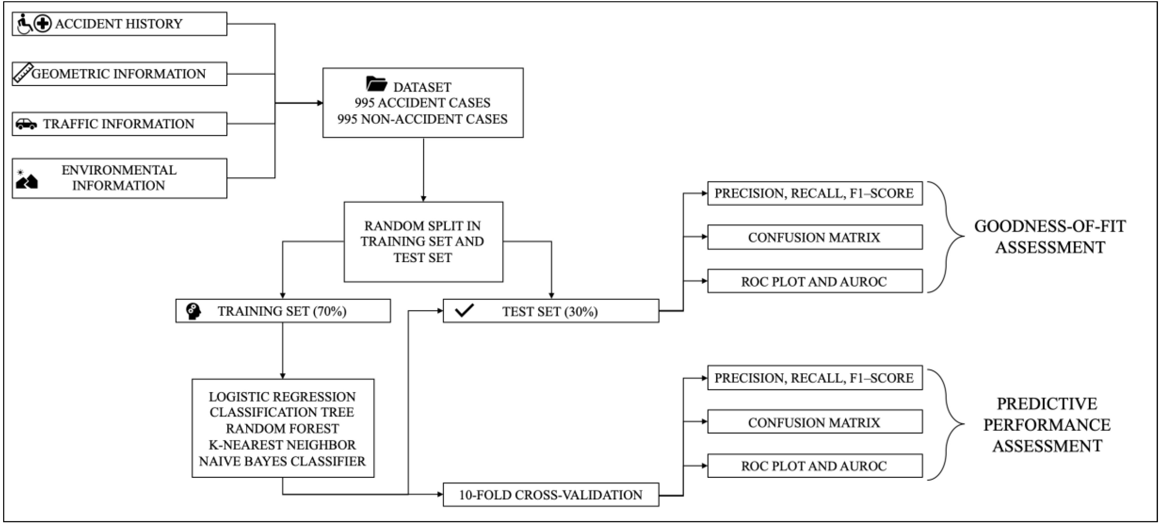
The workflow is shown in the following Figure 1.

Firstly, the following data have been collected from the Tuscany Region Road Administration (TRRA):

• The accident history of the road site analyzed: fatal and injury crashes from 2012 to 2016;
• The geometric data related to the road network: topology, curves and radius, slopes, lane width, type and localization of junctions;
• Traffic flow data: Average Annual Daily Traffic (AADT) for each road analyzed, along with their driveway density;
• Built-up areas information: According to the Italian standards [25] the localization of the built-up areas has been collected in order to discretize the road network into three area types (Road Site Inside an urban area (RSI), Road Site Outside an urban area (RSO), and Road Site on the administrative Boundary of an urban area, (RSB)).

A GIS platform has been exploited in order to match the data collected and define the set of input features (independent variables of the MLAs). According to studies [26,27], the fixed length-based criterion has been chosen for defining the road sites. Therefore, the road network has been discretized into stretches of 500 m, in which each input factor has been computed. Road sites in which at least one accident occurred (an amount of 995) have been classified as “Accident Case”. Subsequently, in order to avoid potential imbalance issues that may affect MLAs [19,28,29], an equal amount of road sites where no accidents occurred in 2012–2016 has been randomly selected. These sites have been labeled as “Non-Accident Case”.

The dataset has been randomly split into two different sets: the training set (70% of the data) and the test set (30%). The training set and a 10-fold Cross-Validation (CV) process have been used for training and evaluating the Goodness-of-Fit of the five MLAs (LR, CART, RF, KNN, NB). The test set has been used for verifying the predictive performance of the algorithms.

In order to evaluate and compare the MLAs, a set of performance metrics has been computed: Precision, Recall, F₁-Score, Confusion Matrices, and AUROC. These metrics should represent the Goodness-of-Fit of the MLAs if they are computed for the training data. Otherwise, if these metrics are computed for the test data, they should represent the predictive performance of the MLAs.

2.2. Data Collection and Database Preparation

2.2.1. Study Area and Input Factors

The network analyzed extends for 1190.136 km (Figure 2). Mainly, it consists of two-lane rural roads. TRAA provided traffic flow data, geometric features, and built-up area characteristics. These data have been employed for the definition of the input factors (or independent variables) of the MLAs.

Accordingly, MLAs have, as input, a set of factors related to the roadway, environment, and traffic. The following list reports the definition of each input factor:

Area Type: Through an overlay of the road network with the urban areas, the road network has been segmented into three different area types:

• RSO (1): road sites completely external to built-up areas;
• RSI (2): road sites completely inside to built-up areas;
• RSB (3): road sites located at the administrative boundaries of built-up areas.

Therefore, the environmental context is represented by a nominal variable that can assume three different values (1, 2, or 3).

Average Annual Daily Traffic:

$${AADT}_J=\frac{1}{n}{\displaystyle \sum }_{i=1}^n{AADT}_{i,j}\left[\frac{veic}{day}\right]$$

(1)

where:

• $n$ is the period, in years, of the analysis, equal to 5 years;
• $AAD{T}_{i,j}$ is the average annual daily traffic for the i-th year evaluated for the j-th road site.

Average carriageway width:

$$W_{c,j}=\frac{ {\sum }_{i=1}^m{W}_{c,i}·L_i}{500}\left[m\right]$$

(2)

where:

• $W_{c,i}$ is the average carriageway width of the i-th segment in the j-th road site;
• $m$ is the number of segments in the j-th road site;
• $L_i$ is the length of the i-th segment.

Average Slope:

$$\overline{I_j }=\frac{{\sum }_{i=1}^m{i}_i·L_i}{500}[\%]$$

(3)

where:

• $i_i$ is the Average Slope of the i-th segment in the j-th road site;
• $m$ is the number of segments in the j-th road site;
• $L_i$ is the length of the i-th segment.

Horizontal Tortuosity Index:

$${HTI}_{,j}=\frac{{\sum }_{i=1}^{r_p}\frac{1}{R_i}}{{\sum }_{i=1}^{r_p}{L}_i}$$

(4)

where:

• $R_i$ is the radius of the i-th circular curve in the j-th road site;
• $r_p$ is the number of elements (circular curves) in the j-th road site;
• $L_i$ is the length of the i-th segment.

Vertical Tortuosity Index:

$${VTI}_j=\frac{{\sum }_{i=1}^{r_v}\frac{1}{{Rv}_i}}{{\sum }_{i=1}^{r_v}{L}_i}$$

(5)

where:

• $R{v}_i$ is the radius of the i-th vertical curve segment in the j-th road site;
• $r_v$ is the number of elements (vertical curves) in the j-th road site;
• $L_i$ is the length of the i-th segment.

Driveway Density:

$${DD}_j=\frac{n_{d,j}}{500}$$

(6)

where:

• $n_{d,j}$ is the number of driveways in the j-th road site.

Density of Road Junctions:

$${DJ}_j=\frac{{{\displaystyle \sum }}_{i=1}^m({\alpha }_i\cdot n_{i,j})}{500}$$

(7)

where:

• ${\alpha }_i$ considers the type of the i-th junction. It can be $\alpha$= 5 for linear signalized and unsignalized intersections, or $\alpha$=1 for roundabouts. The value of $\alpha$ is determined accordingly to Crash Modification Factors reported in Chapter 14, Table 14–3 and Table 14–4 of the HSM [2];
• $n_{i,j}$ is the number of junctions of the i-th type in the j-th road site;
• $m$ is the number of different types of junctions.

The following

Table 2. Input factor and descriptive statistics (training set).

Factor	Statistic	Accident Case	Non-Accident Case
$D{D}_j$	Mean	16.97	7.83
	Std. Dev.	18.19	9.93
$D{J}_j$	Mean	2.90	1.02
	Std. Dev.	3.25	1.76
$VT{I}_j$	Mean	74.54	73.65
	Std. Dev.	71.64	52.7
$\overline{I_j}$	Mean	1.98	1.13
	Std. Dev.	2.80	1.77
$HT{I}_{,j}$	Mean	284.35	384.25
	Std. Dev.	304.84	381.90
$W_{c,j}$	Mean	6.66	6.53
	Std. Dev.	0.66	0.73
$AAD{T}_J$	Mean	8712	4334
	Std. Dev.	5378	3333
AT	RSO–1	348 (38.3%)	560 (61.7%)
	RSI–2	180 (66.7%)	90 (33.3%)
	RSB–3	173 (78.3%)	48 (21.7%)

reports the mean and standard deviation of each input factor belonging to the training set, divided by different classes.

2.2.2. Output Classes

The output response (crash occurrence susceptibility) of the MLAs is a binary categorical variable. Therefore, relying on the input factors mentioned above, MLAs aim to classify a road site as likely safe (by labeling the site as “Non-Accident Case”) or potentially susceptible to an accident occurrence (by labeling the site as “Accident Case”). TRRA provided the crash reports of the Fatal and Injury crashes that occurred on the network over the period 2012–2016. Such crashes:

• Can concern any type of accident (e.g., head-on, run-off, rear-end, side collision, rollover, etc.);
• May have occurred in the day time or night time;
• May have occurred on road segments or road junctions;
• May have involved one or more vehicles;
• May have involved one or more casualties.

Property Damage Only crashes are not included in the dataset since they are not considered by the Italian standards concerning road safety analyses [30].

Certainly, crash reports also record the location of the event. Consequently, through a GIS platform, it was possible to assign the number of accidents that occurred in the five years (2012–2016) of analysis to road sites. If no accidents happened on a road site, it was classified as a “Non-Accident Case”. Conversely, if at least one accident occurred on a road site, the road site was classified as an “Accident Case”. Therefore, the temporal resolution of the crash occurrence predictions of the MLAs is equivalent to five years.

2.3. Machine Learning Algorithms

This part aims to introduce the main characteristics, shortcomings, advantages, and theoretical relations of each MLA employed in this study. All of them are supervised MLAs for classification purposes. Indeed, they are trained with a dataset in which input factors and output classes are known in advance. The purpose of these models is the classification of instances in one of the possible output classes. In order to be compared, all algorithms used the same training and test sets. It is worth mentioning that the Waikato Environment for Knowledge Analysis (WEKA) software [31,32], version 3.8.4, has been employed for building the classifiers.

2.3.1. Logistic Regression

Historically, the LR classifier was defined and employed in the study of Berkson [33]. Firstly, LR exploits a linear multivariate regression for relating the output and the input factors. Accordingly, a logit function is exploited for converting the output of the multivariate linear regression into an output within the range [0,1]. Equation (8) below defines the logit function:

$$\mathrm{P}\left(\mathrm{z}\right)=\frac{1}{{1+\mathrm{e}}^{-\mathrm{z}}}$$

(8)

where:

• $\mathrm{P}\left(\mathrm{z}\right)$ is the probability that the analyzed event occurs; Equation (9) below defines $\mathrm{z}$, that is, the output of regression:

$${\mathrm{z}=\mathrm{b}}_0+{\mathrm{b}}_1{\mathrm{x}}_1+{\mathrm{b}}_2{\mathrm{x}}_2+\dots +{\mathrm{b}}_{\mathrm{m}}{\mathrm{x}}_{\mathrm{m}}$$

(9)

where:

• ${\mathrm{b}}_0$ is a constant term;
• $\mathrm{m}$ is the number of independent variables;
• ${\mathrm{x}}_{\mathrm{i}}$ ($\mathrm{i}$ = 1, 2, 3, …, n) represents the value of the i-th input factor;
• ${\mathrm{b}}_{\mathrm{i}}$ ($\mathrm{i}$ = 1, 2, 3, …, n) is the regression coefficient assigned to the i-th input factor.

LR exploits the following decision rule for assigning new unknown instances to the class $\widehat{z}$ as follows (Equation (10)):

$$\widehat{z} =\{\begin{array}{c}\mathrm{Class}0\mathrm{if}P(z)<0.5\hfill \\ \mathrm{Class}1\mathrm{if}P(z)\ge 0.5\hfill \end{array}$$

(10)

LR provides several advantages to the user:

• It is a widely used technique because it is efficient in terms of training time and computational resources required;
• It is interpretable, providing a non-black-box solution;
• It does not require scaled input features;
• It is easy to train since no hyperparameters have to be tuned.

However, LR has some drawbacks:

• It is not able to solve non-linear problems since its decision surface is linear;
• Since the outcome is discrete, LR can only predict categorical outcomes;
• LR is prone to overfitting issues.

2.3.2. Classification and Regression Tree

CART [34] is a non-parametric MLA used for building a hierarchical tree-based model. The tree starts with a root node, grows through branch nodes, and ends at leaf nodes. Root node and each branch node represent a different decision rule based on a specific input factor: the node is split into two or more homogeneous zones relying on the so-called cut point. The leaf nodes contain the final prediction: in a CART model used for classification, they contain the output class. Therefore, by repeatedly splitting the dataset node-by-node, a tree-based model grows. CART learns decision rules by inferring directly from the training data. It exploits the Recursive Partitioning algorithm [34,35] for identifying the decision rule. For each node, Recursive Partitioning can find the best input feature and the best cut point for splitting the node.

CART model provides a non-black-box solution by a tree-graph visualization. Moreover, CART is not affected by the scale and linear transformation of the input factors, outliers, and insignificant input factors. Last but not least, CART can easily handle numerical and nominal input factors. However, CART models generally suffer overfitting issues by growing over-complex and deep trees. Furthermore, slightly different training sets may lead to significantly different CART.

In order to alleviate these issues, a pruning process of the CART can be used. Pruning is a procedure that leaves out a certain number of hierarchical levels and leaf nodes of the initial CART, making it able to generalize better and perform more reliable prediction. Weka Software provides an automatic pruning process [36,37]. At first, CART developed had 256 decision rules and 257 leaf nodes. After the pruning procedure, CART had 7 decision rules and 8 leaf nodes. Figure 3 below shows the pruned CART.

2.3.3. Random Forest

RF was introduced by Breiman [38]. RF is an ensemble classifier, i.e., it makes classifications relying on different predictions made by a set of individual classifiers: Each of them makes a prediction, then they are averaged in a certain way. In the case of RF, the ensemble classifier consists of a large number of uncorrelated CART models. In order to build uncorrelated classifiers, they are defined by a Bootstrap Aggregation (Bagging) process. Bagging consists of creating a set of different training sets through replacement. Each training set trains each CART of the forest. These CART models are not pruned. Furthermore, a Feature Randomness approach is used in growing trees: Each node is split in branch nodes considering a prefixed number of input factors, selected at random among the whole set [39]. Therefore, by employing Bootstrap Aggregation and Feature Randomness, the RF can exploit the prediction of a large set of uncorrelated CART models. Consequently, RF includes all the strengths of CART. Besides:

• The predictive performance of RF can compete with the best supervised learning algorithms;
• RF can provide a feature importance estimation by the computation of the Out-of-Bag Error;
• Through Bagging and Feature Randomness, RF offers an efficient solution against overfitting.

On the other hand, RF also has a few shortcomings:

• An ensemble model is inherently less interpretable than an individual CART;
• Training a large number of trees may require high computational costs and long training time;
• Predictions are slower than individual classifiers, which may create challenges for some applications.

To classify a new instance, the RF bases its decision rule on the number of times that CART models assign each possible output class to that instance. The class with the maximum number of nominations is assigned to the output class by RF to the new instance.

RF requires that the modeler tunes two hyperparameters: the number of CART models $N_{t }$ to grow and the number of input factors randomly selected $N_{rs}$ as candidates at each split. The “trial and error” approach is widely used in Machine Learning modeling in order to identify the best set of hyperparameters of the algorithms [40,41,42,43,44]. It has been chosen $N_{t }$= 500 CART models since a higher number did not produce a significant increase in RF performance. Moreover, it has been tried $N_{rs}$= 1, 2, …, 8 identifying $N_{rs}=8$ as the better value.

2.3.4. K-Nearest Neighbor

Cover and Hart defined and employed the KNN algorithm at the end of the 1960s [45]. KNN is a supervised instance-based MLA that classify a new sample by considering its k closest instances (called neighbors). To evaluate how close or far an instance is, the KNN algorithm introduces a distance function into the input feature space. The class assigned to the new observation derives directly from the majority class among the k instances considered.

Therefore, KNN requires that the modeler tunes two hyperparameters: the number of the k nearest neighbors and the type of distance function. By following the aforementioned “trial and error” approach, the optimal number of k neighbors has been determined by trying different values of k and computing the Accuracy of the classifier. It has been tried k = 1, 2, 5, 10, 15, 20, and 25. It has been chosen k = 10, considering the highest Accuracy computed. The Euclidean distance defines the distance function. The Euclidean distance $d_{ij}$ between two samples (two points) into the feature space, $i$ and $j$, is defined as Equation (11):

$${\mathrm{d}}_{\mathrm{ij}}=\sqrt[2]{{\displaystyle \sum }_{\mathrm{k}=1}^{\mathrm{m}}{\left({\mathrm{x}}_{\mathrm{ik}}{-\mathrm{x}}_{\mathrm{jk}}\right)}^2}$$

(11)

where:

• m is the dimension of the samples (i.e., the number of independent variables). In this study, m = 8.
• ${\mathrm{x}}_{\mathrm{ik}}$ and ${\mathrm{x}}_{\mathrm{kj}}$ are the values of the k-th input factors for the observation i and j, respectively.

The strengths of KNN are:

• There is no training period: Indeed, KNN does not learn anything in the training period. It does not derive any discriminative function from the training data. KNN stores the training set and learns from it only at the time of making predictions. Accordingly, it makes the KNN algorithm much faster than all the other MLAs;
• Since the KNN algorithm requires no training, new data can be added seamlessly which will not impact the Accuracy of the algorithm;
• KNN is easy to implement; there are only two parameters required to be tuned: the value of K and the distance function (e.g., Euclidean).

The weaknesses of KNN are:

• KNN does not work well with large datasets: The cost of calculating the distance between the new point and each existing point can be high. Therefore, it can degrade the performance of the algorithm;
• KNN does not work well with high dimensional data because it becomes difficult for the algorithm to calculate the distance in each dimension;
• KNN needs feature scaling (standardization and normalization);
• KNN is sensitive to noisy data, missing values, and outliers.

2.3.5. Naïve Bayes Classifier

NB is a probabilistic supervised classifier introduced by Maron [46] in the early 1960s. In order to label a new instance (or feature vector) $x=\left(x_1,\dots ,x_i,\dots x_n\right)$ with one of the possible $k$ output classes $C_k$ of the algorithm, NB exploits the well-known Bayes’ Theorem reported below (Equation (12)):

$$\mathrm{p}\left({\mathrm{C}}_{\mathrm{k}}|{\mathrm{x}}_1{,\dots \mathrm{x}}_{\mathrm{n}}\right)=\mathrm{p}({\mathrm{C}}_{\mathrm{k}}|\mathrm{x})=\frac{{\mathrm{p}(\mathrm{C}}_{\mathrm{k}}\left)·\mathrm{p}(\mathrm{x}|{\mathrm{C}}_{\mathrm{k}}\right)}{\mathrm{p}\left(\mathrm{x}\right)}$$

(12)

where:

• $\mathrm{p}\left({\mathrm{C}}_{\mathrm{k}}|{\mathrm{x}}_1,\dots ,{\mathrm{x}}_{\mathrm{n}}\right)$ is the posterior probability, that is the conditional probability of having the class ${\mathrm{C}}_{\mathrm{k}}$ given the feature vector $x=\left({\mathrm{x}}_1,\dots ,{\mathrm{x}}_{\mathrm{i}},\dots {\mathrm{x}}_{\mathrm{n}}\right)$;
• $\mathrm{p}\left({\mathrm{C}}_{\mathrm{k}}\right)$ is the prior probability of observing an instance belonging to the class ${\mathrm{C}}_{\mathrm{k}}$. Since the dataset is balanced and composed of two classes, $\mathrm{p}\left({\mathrm{C}}_{\mathrm{k}}\right)=0.5$;
• $\mathrm{p}\left(x|{\mathrm{C}}_{\mathrm{k}}\right)$ is the conditional probability of observing the feature vector $x$ given the output class ${\mathrm{C}}_{\mathrm{k}}$;
• $\mathrm{p}\left(x\right)$ is the probability of observing the feature vector $x$, and it is common to all classes.

By assuming that all the features in $x$ are mutually independent (Naïve condition), and repeating the application of the concept of conditional probabilities (chain rule), the numerator of Equation (12) becomes Equation (13):

$$\mathrm{p}\left({\mathrm{C}}_{\mathrm{k}}\right)·\mathrm{p}\left(\mathrm{x}|{\mathrm{C}}_{\mathrm{k}}\right)=\mathrm{p}\left({\mathrm{C}}_{\mathrm{k}}\right)·{\displaystyle \prod }_{\mathrm{i}=1}^{\mathrm{n}}\mathrm{p}\left({\mathrm{x}}_{\mathrm{i}}|{\mathrm{C}}_{\mathrm{k}}\right)$$

(13)

Therefore, the decision rule of NB classifiers that assign a class $\widehat{z}$ to a new instance is defined as follows (Equation (14)):

$$\widehat{z}=\underset{k\in \{1,\dots ,K\}}{\text{argmax}}\mathrm{p}\left({\mathrm{C}}_{\mathrm{k}}\right)·{\displaystyle \prod }_{\mathrm{i}=1}^{\mathrm{n}}\mathrm{p}\left({\mathrm{x}}_{\mathrm{i}}|{\mathrm{C}}_{\mathrm{k}}\right)$$

(14)

Equation (14) is called a Maximum a Posteriori decision rule: NB computes the probability that a new instance belongs to any different output classes, then it assigns the class considering the highest probability.

NB has several advantages:

• It is easy to train since no hyperparameters have to be tuned;
• It is fast in predicting the classes of the sample belonging to the test set;
• It requires less training data compared to the LR for training a reliable classifier.

However, NB has some limitations:

• If a categorical variable (e.g., Area Type) has a category in the test set which was not observed in the training set, then the model assigns a zero probability to the event occurrence and will be unable to make a reliable prediction. This issue is known as “Zero Frequency”. Accordingly, the CV procedure is essential for ensuring that all the categories of the categorical variables have been considered in both the training and test sets;
• For numerical variables (e.g., AADT), the NB makes the strong assumption that they are distributed according to the normal distribution;
• Generally, it is almost impossible that the predictors of a phenomenon are entirely independent.

2.3.6. Modeling Settings

This section reports the main procedural steps common to all MLAs.

Set up of the dataset: The initial dataset contains an equal number of “Accident Case” and “Non-Accident Case” sites, considering the possible weakness in the prediction of the minority class by classifiers trained on unbalanced training sets. Therefore, once all the sites where accidents occurred have been taken into consideration, an equal number of “Non-Accident Case” road sites have been randomly extracted from the network.

Definition of the training and test set: The initial dataset has been randomly divided into two distinct sets, one for training the models and the other for testing them. As other authors did [47,48,49,50], we chose percentages equal to 70% of the initial dataset for training MLAs and 30% for testing them.

K-fold CV approach: In order to verify that the models are robust and reliable in their predictions, they have been evaluated through a 10-fold CV process. The CV has been introduced by Larson [51], who defined the concept of splitting the dataset into two parts and then using one for training the model and the other one for judging it. Subsequently, Mosteller and Tukey [52] proposed the k-fold CV procedure adopted in this study. The process of k-fold CV consists of splitting the training set into k-folds. Afterward, at iteration k, k − 1 folds are used for training the model, and the leaved-out fold for evaluating it. After k iterations, all the samples belonging to the training set are used both for training and evaluating the MLA, ensuring the most representative evaluation of the algorithm. In this study, as recommended by Kohavi [53], a 10-fold CV has been followed.

Assessment of training and test phases: Both phases have been evaluated with the same type of metrics: overall Accuracy, Precision, Recall, F1-Score, Confusion Matrix, ROC, and AUROC. These metrics allow judging the quality of the models (if they suffer from overfitting problems), and therefore the predictive performance in classifying an unknown instance.

2.4. Evaluation Metrics

A comprehensive set of performance metrics has been used for the evaluation of the MLAs. The following Equations (15)–(18) define the overall Accuracy of the classifiers, Precision, Recall, and F1-Score, respectively.

$$\mathrm{Accuracy}=\frac{\mathrm{TP}+\mathrm{TN}}{\mathrm{TP}+\mathrm{FP}+\mathrm{TN}+\mathrm{FN}}$$

(15)

$$\mathrm{Precision}=\frac{\mathrm{TP}}{\mathrm{TP}+\mathrm{FP}}$$

(16)

$$\mathrm{Recall}=\frac{\mathrm{TP}}{\mathrm{TP}+\mathrm{FN}}$$

(17)

$${\mathrm{F}}_1=\frac{2}{\frac{1}{\mathrm{Precision}}+\frac{1}{\mathrm{Recall}}}=\frac{\mathrm{TP}}{\mathrm{TP}+\frac{\mathrm{FN}+\mathrm{FP}}{2}}$$

(18)

where:

• TP is the number of True Positive instances, i.e., the instances belonging to the class “Accident Case” classified into the same class;
• TN is the number of True Negative instances, i.e., the instances belonging to the class “Non-Accident Case” classified into the same class;
• FP is the number of False Positive instances, i.e., the instances belonging to the class “Non-Accident Case” misclassified into “Accident Case”;
• FN is the number of False Negative instances, i.e., the instances belonging to the class “Accident Case” misclassified into class “Non-Accident Case”.

If the dataset is balanced, the overall Accuracy should represent the global performance of the classifier accurately. The Precision shows the goodness of positive predictions. The higher is the Precision, and the lower is the number of “False Alarms”. The Recall, also called True Positive Rate (TPR), is the ratio of positive instances that are correctly detected by the classifier. Therefore, the higher the Recall, the higher is the quality of the classifier in detecting positive instances. The F₁-Score is the harmonic mean of Precision and Recall, and it can be used for comparing classifiers since they are combined into a concise metric. The harmonic mean is used instead of the arithmetic one since it is more susceptible to low values. Therefore, a valid classifier has a satisfactory F₁-Score only if it has high Precision and high Recall. These parameters can be computed as specific metrics for each class or as the overall metrics of the classifier.

Furthermore, MLAs have been judged and compared by computing the Confusion Matrix and the AUROC. The Confusion Matrix reports the TP, TN, FP, and FN instances as a two-by-two matrix, in which the rows correspond to the observed classes, while the columns correspond to the predicted ones. An adequate Confusion Matrix has the most of the instances on its main diagonal. Furthermore, by observing a Confusion Matrix, it is possible to compute the performance metrics mentioned above. The Receiver Operating Characteristic (ROC) curve represents the performance of a classifier onto a cartesian plane. The TPR is reported on the ordinates, while the abscissas show the False Positive Rate (FPR). Equation (19) defines the FPR:

$$\mathrm{FPR}=\frac{\mathrm{FP}}{\mathrm{FP}+\mathrm{TN}}$$

(19)

Therefore, the FPR is the ratio of FP instances among all negative instances, i.e., the ratio of “False Alarms” given by the classifier. The ROC plot shows the relation between TPR and FPR at various classification thresholds. Once the ROC is plotted, the Area Under the ROC (AUROC) [54] can be computed. It is the two-dimensional area underneath the ROC curve [16]. Hypothetically, it can assume values between 0 and 1. The value of 0.5 represents a random classifier, while the value of 1 represents the perfect classifier that classifies each sample into the right class. Therefore, the higher is the AUROC, the better is the classifier.

3. Results and Discussion

Outcomes are presented and discussed in terms of Goodness-of-Fit and predictive performance. Goodness-of-Fit refers to the quality of the training phase, while predictive performance represents the ability of the MLAs to be able to generalize (test phase). We provided detailed performance metrics for each class of the classification (Accident and Non-Accident class) and the weighted average values, i.e., the average value of each performance metric weighted by the number of samples for each class. These averaged metrics represent the overall performance of the classifiers.

Firstly, Precision, Recall, and F1-Score are introduced for the evaluation of both Goodness-of-Fit and predictive performance. Afterward, the Confusion Matrix of each classifier (both in training and testing phase) and the Accuracy are shown. Finally, the ROC plots are reported, and the AUROC computed (both in the training and testing phase).

3.1. Precision, Recall, F1-Score

Table 3. Precision, Recall, and F₁-Score of MLAs in the training phase.

Model	LR			CART			RF			KNN			NB
Class	Prec.	Rec.	F1	Prec.	Rec.	F1	Prec.	Rec.	F1	Prec.	Rec.	F1	Prec.	Rec.	F1
Accident Case	0.769	0.610	0.681	0.747	0.672	0.707	0.742	0.668	0.703	0.680	0.685	0.682	0.786	0.532	0.634
Non-Accident Case	0.676	0.816	0.739	0.701	0.771	0.734	0.697	0.767	0.730	0.681	0.676	0.679	0.645	0.855	0.735
Weighted Average	0.722	0.713	0.710	0.724	0.721	0.721	0.719	0.717	0.716	0.681	0.681	0.681	0.716	0.693	0.685

below shows Precision, Recall, and F1-Score of MLAs computed for the Goodness-of-Fit assessment.

Both the weighted average metrics and the specific ones for each class seem satisfactory. The highest Precision (0.786) is showed by the NB classifier in detecting Accident Case road sites, while LR reports the highest Recall (0.816) in recognizing Non-Accident Case road sites. Since the dataset is balanced, the Weighted Average metrics should assume an adequate representation of the real performance of a classifier. In this case, the highest Precision (0.724) and the highest Recall have been observed (0.721) for the CART algorithm. Accordingly, F1-Score shows the best value (0.721) for the CART algorithm.

Table 4. Precision, Recall, and F₁-Score of MLAs in the testing phase.

Model	LR			CART			RF			KNN				NB
Class	Prec.	Rec.	F1	Prec.	Rec.	F1	Prec.	Rec.	F1	Prec.	Rec.	F1	Prec.		Rec.	F1
Accident Case	0.731	0.650	0.688	0.754	0.630	0.686	0.746	0.710	0.728	0.680	0.667	0.673	0.758		0.529	0.623
Non-Accident Case	0.688	0.763	0.724	0.685	0.797	0.737	0.726	0.760	0.743	0.676	0.690	0.683	0.641		0.833	0.725
Weighted Average	0.709	0.707	0.706	0.719	0.714	0.712	0.736	0.735	0.735	0.678	0.678	0.678	0.699		0.682	0.674

below reports Precision, Recall, and F1-Score of MLAs computed in the testing phase. As well as in the training phase, Table 4 demonstrates that in the testing phase, the MLAs present adequate predictive capacities. Qualitatively, the whole set of metrics is similar to the one shown in the previous Table 3; therefore, the fact that these MLAs do not suffer from overfitting issues should be ensured. Quantitatively, NB reports the highest Precision (0.758) in detecting Accident Case road sites and the highest Recall (0.833) in identifying Non-Accident Case road sites. Nonetheless, the classifier that presents the best weighted average metrics is the RF algorithm. Indeed, the highest Precision (0.736), the highest Recall (0.735), and the highest F1-Score (0.735) have been observed for the RF.

By employing Precision, Recall, and F1-Score for evaluating the Goodness-of-Fit and predictive performance, it is confirmed that RF is the most appropriate one for predicting road blackspots. The other MLAs also showed satisfactory performance and, therefore, should be considered as different alternatives to the RF.

3.2. Confusion Matrices

Table 5. Confusion Matrices of MLAs in training phase: LR, CART, RF, KNN, and NB.

Predicted		LR Training Phase
Accident Case	Non-Accident Case
426	272	Accident Case	Observed
128	567	Non-Accident Case
Correctly Classified Instances: 993 (71.29%)
Incorrectly Classified Instances: 400 (28.72%)
Predicted		CART Training Phase
Accident Case	Non-Accident Case
469	229	Accident Case	Observed
159	536	Non-Accident Case
Correctly Classified Instances: 1005 (72.15%)
Incorrectly Classified Instances: 388 (27.85%)
Predicted		RF Training Phase
Accident Case	Non-Accident Case
466	232	Accident Case	Observed
162	533	Non-Accident Case
Correctly Classified Instances: 999 (71.72%)
Incorrectly Classified Instances: 394 (28.28%)
Predicted		KNN Training Phase
Accident Case	Non-Accident Case
478	220	Accident Case	Observed
225	470	Non-Accident Case
Correctly Classified Instances: 948 (68.05%)
Incorrectly Classified Instances: 445 (31.95%)
Predicted		NB Training phase
Accident Case	Non-Accident Case
371	327	Accident Case	Observed
101	594	Non-Accident Case
Correctly Classified Instances: 965 (69.27%)
Incorrectly Classified Instances: 428 (30.73%)

below reports the Confusion Matrices computed after the training phase of the MLAs. At the bottom of each Confusion Matrix, it is reported the number of correctly classified instances (that is, the overall Accuracy of the classifier), and the number of incorrectly classified instances.

As regards to the Accident Case class, the Confusion Matrices demonstrate that KNN is the most suitable classifier (478 instances out of 698 samples correctly classified). The NB is the best classifier in detecting Non-Accident Cases (594 out of 695). The highest overall Accuracy (72.15%) is shown by the CART algorithm, with 1005 instances out of 1393 samples correctly classified.

Table 6. Confusion Matrices of MLAs in the testing phase: LR, CART, RF, KNN, and NB.

Predicted		LR Testing Phase
Accident Case	Non-Accident Case
193	104	Accident Case	Observed
71	229	Non-Accident Case
Correctly Classified Instances: 422 (70.69%)
Incorrectly Classified Instances: 175 (29.31%)
Predicted		CART Testing Phase
Accident Case	Non-Accident Case
187	110	Accident Case	Observed
61	239	Non-Accident Case
Correctly Classified Instances: 426 (71.35%)
Incorrectly Classified Instances: 171 (28.65%)
Predicted		RF Testing Phase
Accident Case	Non-Accident Case
211	86	Accident Case	Observed
72	228	Non-Accident Case
Correctly Classified Instances: 439 (73.53%)
Incorrectly Classified Instances: 158 (26.47%)
Predicted		KNN Testing Phase
Accident Case	Non-Accident Case
198	99	Accident Case	Observed
93	207	Non-Accident Case
Correctly Classified Instances: 405 (67.84%)
Incorrectly Classified Instances: 192 (32.16%)
Predicted		NB Testing Phase
Accident Case	Non-Accident Case
157	140	Accident Case	Observed
50	250	Non-Accident Case
Correctly Classified Instances: 407 (68.17%)
Incorrectly Classified Instances: 190 (31.83%)

below shows the predictive performance of the MLAs by the Confusion Matrices computed after the testing phase.

The RF classifier predicts the highest number of Accident Cases (211 instances out of 297). The Non-Accident Cases are better classified by NB (250 out of 300). The highest overall Accuracy (73.53%) is shown by the RF algorithm, with 439 instances out of 597 samples correctly classified. Once evaluating the algorithms by the Confusion Matrix, the RF seems to be the most reliable one.

3.3. ROC and AUROC

In order to judge the MLAs comprehensively, the ROC is derived for each classifier. ROC has been plotted for both the training and testing phases (Figure 4 and Figure 5, respectively). For each ROC, the corresponding AUROC (

Table 7. AUROC of the algorithms: Training and test phase.

Model	LR	CART	RF	KNN	NB
AUROC training phase	0.766	0.763	0.783	0.757	0.749
AUROC test phase	0.773	0.742	0.795	0.740	0.747

) has been computed. These outcomes are presented below.

The dash-dot line in Figure 4 represents the performance of a hypothetical random classifier, which corresponds to an AUROC of 0.5. Therefore, the further a ROC is far away from this line, the better the algorithm. Qualitatively, Figure 4 reports that both in Accident and Non-Accident Cases, all MLAs have similar trends in the TPR–FPR space.

Figure 5 below reports the ROC for the test phase of MLAs.

Once again, all MLAs show similar trends and similar ROC to the ones derived for the training phase. This fact should ensure that the modeling procedure has been carried out correctly.

As said, for a quantitative assessment with the use of ROC curves, the AUROC values need to be computed. Table 7 below reports the values of AUROC for each classifier, both in the training and test phase. Considering that the dataset is balanced, it is worth mentioning that the AUROC of MLAs for detecting Accident and Non-Accident classes assume the same value. Therefore, Table 7 distinguish MLAs only between training and test phases.

By observing Table 7, it is shown that AUROC in the training and test phases assume similar values. This fact should confirm that the MLAs calibrated do not suffer from overfitting. For the data used in this work, RF is the most reliable and suitable algorithm in predicting road blackspots (AUROC of the test phase = 0.795), followed by LR (0.773), NB (0.747), CART (0.742), and KNN (0.740). These values also indicate that the other MLAs used in this study can be useful for reaching the purpose. Moreover, the predictive performance of the MLAs shown in Table 7 for the test set are consistent with those presented in Table 4 and Table 6.

4. Conclusions

A road blackspot screening procedure based on real long-term traffic data and machine learning algorithms has been presented. This process aims to classify a road site as safe or potentially susceptible to an accident occurrence.

In order to fulfill the objective of this study, five different supervised classification algorithms have been calibrated and compared. Specifically, an instance-based algorithm (KNN), two probabilistic models (LR and NB), a non-parametric tree-based algorithm (CART), and a non-parametric ensemble classifier (RF), have been employed. Both the training and the test phase have been judged by computing a broad set of performance metrics: Precision, Recall, F1-Score, overall Accuracy, Confusion Matrix, and AUROC. Considering that both phases provided satisfactory and similar performance among all these metrics, it is proved that the algorithms should not suffer from overfitting issues. Moreover, considering that the Random Forest classifier showed the highest performance in all the test phase-related metrics (F1-Score = 0.735, overall Accuracy = 73.53%, and AUROC = 0.795), we recommend such a classifier as reliable and suitable algorithms in road blackspot detection modeling. Furthermore, all the other algorithms offer adequate performance as well, and they may be more accurate than Random Forest in other similar researches. Therefore, it is also essential to calibrate and compare different algorithms for ensuring that one of the possible best solutions has been found out.

Road Authorities should consider the use of Machine Learning classifiers for the prediction of the safety level of the road networks they manage. These procedures can efficiently be employed as a supporting tool in decision-making processes concerning road maintenance intervention and planning new road projects. Indeed, such algorithms allow predicting the dangerousness of new road sites, as well as of road sites that have not yet experienced a long-term crash history. Once the screening procedure is terminated, a restricted sample of road sites is highlighted as potentially susceptible to crash occurrence. These sites could be included appropriately by Road Authorities in inspection lists with higher priority.

References

- World Health Organization. Global Status Report on Road Safety 2018: Summary 2018; World Health Organization: Geneva, Switzerland, 2018. [Google Scholar]
- American Association of State Highway and Transportation Officials. Highway Safety Manual, 1st ed.; American Association of State Highway and Transportation Officials: Washington, DC, USA, 2010. [Google Scholar]
- Farid, A.; Abdel-Aty, M.; Lee, J. Transferring and calibrating safety performance functions among multiple States. Accid. Anal. Prev. 2018. [Google Scholar] [CrossRef] [PubMed]
- Wang, K.; Zhao, S.; Jackson, E. Functional forms of the negative binomial models in safety performance functions for rural two-lane intersections. Accid. Anal. Prev. 2019, 124, 193–201. [Google Scholar] [CrossRef] [PubMed]
- Fiorentini, N.; Losa, M. Developing Safety Performance Functions for Facilities by Environmental Context on Italian Two-Lane Rural Roads. Saf. Sci. 2020. under review. [Google Scholar]
- Hauer, E. Observational Before/After Studies in Road Safety. In Estimating the Effect of Highway and Traffic Engineering Measures on Road Safety; Emerald Group Publishing: Bingley, UK, 1997. [Google Scholar]
- Lee, J.; Chung, K.; Kang, S. Evaluating and addressing the effects of regression to the mean phenomenon in estimating collision frequencies on urban high collision concentration locations. Accid. Anal. Prev. 2016, 97, 49–56. [Google Scholar] [CrossRef] [PubMed]
- Brimley, B.; Saito, M.; Schultz, G. Calibration of highway safety manual safety performance function. Transp. Res. Rec. 2012. [Google Scholar] [CrossRef]
- Ghadi, M.; Török, Á. A comparative analysis of black spot identification methods and road accident segmentation methods. Accid. Anal. Prev. 2019, 128, 1–7. [Google Scholar] [CrossRef]
- Dogru, N.; Subasi, A. Traffic accident detection using random forest classifier. In Proceedings of the 2018 15th Learning and Technology Conference, L and T 2018, Jeddah, Saudi Arabia, 25–26 February 2018; Institute of Electrical and Electronics Engineers Inc.: Piscataway, NJ, USA, 2018; pp. 40–45. [Google Scholar]
- Xiao, J. SVM and KNN ensemble learning for traffic incident detection. Phys. A Stat. Mech. Appl. 2019, 517, 29–35. [Google Scholar] [CrossRef]
- Xiao, J.; Liu, Y. Traffic incident detection using multiple-kernel support vector machine. Transp. Res. Rec. 2012, 2324, 44–52. [Google Scholar] [CrossRef]
- You, J.; Wang, J.; Guo, J. Real-time crash prediction on freeways using data mining and emerging techniques. J. Mod. Transp. 2017, 25, 116–123. [Google Scholar] [CrossRef]
- Hossain, M.; Muromachi, Y. A Bayesian network based framework for real-time crash prediction on the basic freeway segments of urban expressways. Accid. Anal. Prev. 2012, 45, 373–381. [Google Scholar] [CrossRef]
- Basso, F.; Basso, L.J.; Bravo, F.; Pezoa, R. Real-time crash prediction in an urban expressway using disaggregated data. Transp. Res. Part C Emerg. Technol. 2018. [Google Scholar] [CrossRef]
- Li, P.; Abdel-Aty, M.; Yuan, J. Real-time crash risk prediction on arterials based on LSTM-CNN. Accid. Anal. Prev. 2020. [Google Scholar] [CrossRef] [PubMed]
- Yuan, J.; Abdel-Aty, M.A.; Gong, Y.; Cai, Q. Real-Time Crash Risk Prediction using Long Short-Term Memory Recurrent Neural Network. Transp. Res. Rec. J. Transp. Res. Board 2019, 2673, 314–326. [Google Scholar] [CrossRef]
- Lv, Y.; Tang, S.; Zhao, H.; Li, S. Real-time highway accident prediction based on support vector machines. In Proceedings of the 2009 Chinese Control and Decision Conference (CCDC), Guilin, China, 17–19 June 2009; pp. 4403–4407. [Google Scholar] [CrossRef]
- Schlögl, M.; Stütz, R.; Laaha, G.; Melcher, M. A comparison of statistical learning methods for deriving determining factors of accident occurrence from an imbalanced high resolution dataset. Accid. Anal. Prev. 2019, 127, 134–149. [Google Scholar] [CrossRef] [PubMed]
- Theofilatos, A.; Chen, C.; Antoniou, C. Comparing Machine Learning and Deep Learning Methods for Real-Time Crash Prediction. Transp. Res. Rec. 2019, 2673, 169–178. [Google Scholar] [CrossRef]
- Xiao, J.; Liu, Y. Traffic incident detection by multiple kernel support vector machine ensemble. In Proceedings of the IEEE Conference on Intelligent Transportation Systems, ITSC, Anchorage, AK, USA, 16–19 September 2012; pp. 1669–1673. [Google Scholar]
- Mokhtarimousavi, S.; Anderson, J.C.; Azizinamini, A.; Hadi, M. Improved Support Vector Machine Models for Work Zone Crash Injury Severity Prediction and Analysis. Res. Artic. Transp. Res. Rec. 2019, 2673, 680–692. [Google Scholar] [CrossRef]
- Wahab, L.; Jiang, H. Severity prediction of motorcycle crashes with machine learning methods. Int. J. Crashworth. 2019, 1–8. [Google Scholar] [CrossRef]
- Iranitalab, A.; Khattak, A. Comparison of four statistical and machine learning methods for crash severity prediction. Accid. Anal. Prev. 2017, 108, 27–36. [Google Scholar] [CrossRef]
- Nuovo Codice della Strada. 1992. Available online: http://www.mit.gov.it/mit/site.php?p=normativa&o=vd&id=1&id_cat=&id_dett=0, (accessed on 10 May 2020).
- Cafiso, S.; D’Agostino, C.; Persaud, B. Investigating the influence of segmentation in estimating safety performance functions for roadway sections. J. Traffic Transp. Eng. 2018. [Google Scholar] [CrossRef]
- Koorey, G. Road Data Aggregation and Sectioning Considerations for Crash Analysis. Transp. Res. Rec. J. Transp. Res. Board 2009. [Google Scholar] [CrossRef]
- Fiorentini, N.; Losa, M. Handling Imbalanced Data in Road Crash Severity Prediction by Machine Learning Algorithms. Infrastructures 2020, 5, 61. [Google Scholar] [CrossRef]
- He, H.; Garcia, E.A. Learning from imbalanced data. IEEE Trans. Knowl. Data Eng. 2009. [Google Scholar] [CrossRef]
- Linee Guida per la Gestione della Sicurezza Delle Infrastrutture Stradali ai Sensi dell’art. 8 del Decreto Legislativo 15 Marzo 2011. 2012. Available online: http://www.mit.gov.it/documentazione/il-decreto-legislativo-n-352011-adozione-delle-linee-guida-per-la-gestione-della. (accessed on 10 May 2020).
- Witten, I.H.; Frank, E.; Hall, M.A.; Pal, C.J. The WEKA Workbench. Online Appendix for “Data Mining: Practical Machine Learning Tools and Techniques”; Morgan Kaufmann: Burlington, MA, USA, 2016. [Google Scholar]
- Hall, M.; Frank, E.; Holmes, G.; Pfahringer, B.; Reutemann, P.; Witten, I.H. The WEKA data mining software. ACM SIGKDD Explor. Newsl. 2009, 11, 10–18. [Google Scholar] [CrossRef]
- Berkson, J. Application of the Logistic Function to Bio-Assay. J. Am. Stat. Assoc. 1944. [Google Scholar] [CrossRef]
- Breiman, L.; Friedman, J.H.; Olshen, R.A.; Stone, C.J. Classification and Regression Trees; CRC Press: Belmont, CA, USA, 1984. [Google Scholar]
- Loh, W.-Y.; Shih, Y.-S. Split selection methods for classification trees. Stat. Sin. 1997, 7, 815–840. [Google Scholar]
- Patel, N.; Upadhyay, S. Study of Various Decision Tree Pruning Methods with their Empirical Comparison in WEKA. Int. J. Comput. Appl. 2012, 60, 20–25. [Google Scholar] [CrossRef]
- Rajesh, P.; Karthikeyan, M.A. Comparative Study of Data Mining Algorithms for Decision Tree Approaches using WEKA Tool. Adv. Nat. Appl. Sci. 2017, 11, 230–243. [Google Scholar]
- Breiman, L. Random forests. Mach. Learn. 2001. [Google Scholar] [CrossRef]
- Pfahringer, B. Random Model Trees: An Effective and Scalable Regression Method; University of Waikato: Waikato, New Zealand, 2010. [Google Scholar]
- Zhang, J.; Li, Z.; Pu, Z.; Xu, C. Comparing prediction performance for crash injury severity among various machine learning and statistical methods. IEEE Access 2018. [Google Scholar] [CrossRef]
- Fernández-Delgado, M.; Cernadas, E.; Barro, S.; Amorim, D.; Fernández-Delgado, A. Do we need hundreds of classifiers to solve real world classification problems? J. Mach. Learn. Res. 2014, 15, 3133–3181. [Google Scholar]
- Bergstra, J.; Bengio, Y. Random Search for Hyper-Parameter Optimization. J. Mach. Learn. Res. 2012, 13, 281–305. [Google Scholar]
- Delen, D.; Tomak, L.; Topuz, K.; Eryarsoy, E. Investigating injury severity risk factors in automobile crashes with predictive analytics and sensitivity analysis methods. J. Transp. Health 2017, 4, 118–131. [Google Scholar] [CrossRef]
- Olutayo, V.A.; Eludire, A.A. Traffic Accident Analysis Using Decision Trees and Neural Networks. Inf. Technol. Comput. Sci. 2014, 2, 22–28. [Google Scholar] [CrossRef]
- Cover, T.M.; Hart, P.E. Nearest Neighbor Pattern Classification. IEEE Trans. Inf. Theory 1967, 13, 21–27. [Google Scholar] [CrossRef]
- Maron, M.E. Automatic Indexing: An Experimental Inquiry. J. ACM 1961, 8, 404–417. [Google Scholar] [CrossRef]
- Al Mamlook, R.E.; Kwayu, K.M.; Alkasisbeh, M.R.; Frefer, A.A. Comparison of machine learning algorithms for predicting traffic accident severity. In Proceedings of the 2019 IEEE Jordan International Joint Conference on Electrical Engineering and Information Technology (JEEIT), Amman, Jordan, 9–11 April 2019; pp. 272–276. [Google Scholar] [CrossRef]
- Abdel-Aty, M.; Haleem, K. Analyzing angle crashes at unsignalized intersections using machine learning techniques. Accid. Anal. Prev. 2011, 43, 461–470. [Google Scholar] [CrossRef]
- Yu, B.; Wang, Y.T.; Yao, J.B.; Wang, J.Y. A comparison of the performance of ann and svm for the prediction of traffic accident duration. Neural Netw. World 2016, 26, 271. [Google Scholar] [CrossRef]
- Tang, H.; Donnell, E.T. Application of a model-based recursive partitioning algorithm to predict crash frequency. Accid. Anal. Prev. 2019, 132, 105274. [Google Scholar] [CrossRef]
- Larson, S.C. The shrinkage of the coefficient of multiple correlation. J. Educ. Psychol. 1931, 22, 45–55. [Google Scholar] [CrossRef]
- Mosteller, F.; Tukey, J.W. Data Analysis, Including Statistics. In The Handbook of Social Psychology; Addison-Welsey: Boston, MA, USA, 1968; Volume 2, pp. 80–203. [Google Scholar]
- Kohavi, R. A Study of Cross-Validation and Bootstrap for Accuracy Estimation and Model Selection. In Proceedings of the International Joint Conference on Artificial Intelligence, Montreal, QC, Canada, 20–25 August 1995; pp. 1137–1145. [Google Scholar]
- Hanley, J.A.; McNeil, B.J. The meaning and use of the area under a receiver operating characteristic (ROC) curve. Radiology 1982. [Google Scholar] [CrossRef]
© 2020 by the authors. Licensee MDPI, Basel, Switzerland. This article is an open access article distributed under the terms and conditions of the Creative Commons Attribution (CC BY) license (http://creativecommons.org/licenses/by/4.0/).