1. Introduction
Studies showing that income inequality plays a constructive role in sustainable economic growth (positive theory) and studies showing a negative role (negative theory) seem to reach mutually contradictory conclusions. Ref. [
1] is a typical study emphasizing an active role of income inequality in economic growth. In his paper “Equality and Efficiency: The Big Trade-off”, Okun argues that income inequality, by giving appropriate motivations to economic agents, promotes labor willingness, capital accumulation and technological innovation, thus resulting in aggressive economic growth. In the same context, Okun indicates that welfare institutions and redistribution policies create distortions, such as the “leaky bucket”, such that income redistribution policy is predicted to have a negative influence on economic efficiency and economic growth. In recent years, Ref. [
2] have found that income inequality plays an active role in technological innovation and entrepreneurial spirit in a comparison study of the United States and Sweden.
However, since the global financial crisis, further studies have highlighted the negative impact of income inequality on growth. Looking at the global financial crisis, the worst since the Great Depression of the 1930s, economists have begun to raise questions about Okun’s trade-off between equality and efficiency and have focused on the linkages among income inequality, increased systemic instability, and low economic growth. As a result, they have reached the following conclusions. First, it is clear that waves of growth have not “floated all boats”. The steady state assumed by Solow and trickle-down effects have failed to resolve income inequality in the process of economic growth. Rather, widening income inequality threatens economic sustainability and causes economic crises [
3,
4,
5]. Secondly, researchers point out that the expansion of income inequality was one cause of the global financial crisis [
4,
5,
6,
7]. Third, more focus has been directed at the importance of political factors in increasing income inequality [
8,
9].
In this study, we construct a theoretical model that covers both the positive and negative arguments. Based on this, we empirically test the effects of income inequality on economic growth using macro data for 43 countries. Past studies have shown that income inequality has a significant impact on technological innovation, investment, and accumulation of human capital. As a result, income inequality has been attracting attention as a channel through which economic growth is impacted. The model of income inequality we propose in this paper has been developed to consider the possibility of both positive and negative impacts of income inequality on technological innovation, investment, and the accumulation of human capital. This allows us to investigate how income inequality has a positive or negative impact on sustainable economic growth. Next, we test the cumulative growth model by using macro data from 43 countries, along with country dummy variables such as developed/developing countries and Asian/South American countries. Finally, based on the results, we examine what types of government policies should be followed in relation to growing income inequality and how these policies could affect income inequality growth.
This paper is organized as follows. In
Section 2, we review the extant literature. In
Section 3, we construct a model showing the correlation between income inequality and growth. In
Section 4, we present the empirical estimation results, and in
Section 5, we conclude the paper.
2. Literature Review
Studies showing that income inequality plays a positive role in economic growth are largely based on three arguments. The first argument focuses on investment indivisibilities wherein large sunk costs are required when implementing new fundamental innovations. Without stock markets and financial institutions to mobilize large sums of money, a high concentration of wealth is needed for individuals to undertake new industrial activities accompanied by high sunk costs [
1,
10,
11]. supporting [
10,
12] shows the relation between economic growth and income inequality for 45 countries during 1966–1995. He finds out that the increase in income inequality has a significant positive relationship with economic growth in the short and medium term. Using system GMM, [
13] estimate the relation between income inequality and economic growth for 106 countries during 1965–2005 period. The results show that income inequality has a positive impact on economic growth in the short run, but the two are negatively correlated in the long run. The second argument is related to moral hazard and incentives, and was first modeled by [
14]. Because economic performance is determined by the unobservable level of effort that agents make, paying compensations without taking into account the economic performance achieved by individual agents will fail to elicit optimum effort from the agents. Thus, certain income inequalities contribute to growth by enhancing worker motivation [
1] and by giving motivation to innovators and entrepreneurs [
15]. Finally, [
16] point out that the concentration of wealth or stock ownership in relation to corporate governance contributes to growth. If stock ownership is distributed and owned by a large number of shareholders, it is not easy to make quick decisions due to the conflicting interests among shareholders, and this may also cause a free-rider problem in terms of monitoring and supervising managers and workers. This line of reasoning is commonly found in research asserting the need for asset ownership and concentration of wealth in Central and Eastern European countries and other transition economies and is related to the so-called “tragedy of the anti-commons” of [
17].
Various studies have examined the relationships between income inequality and economic growth, and most of these assert that a negative correlation exists between the two. In particular, recent studies include [
18]. Analyzing 159 countries for 1980–2012, they conclude that there exists a negative relation between income inequality and economic growth; when the income share of the richest 20% of population increases by 1%, the GDP decreases by 0.08%, whereas when the income share of the poorest 20% of population increases by 1%, the GDP increases by 0.38%. Some studies find that inequality has a negative impact on growth due to poor human capital accumulation and low fertility rates [
19,
20,
21,
22], while [
23,
24] point out that inequality creates political instability, resulting in lower investment. [
25,
26] argue that widening income inequality has a negative impact on economic growth because it negatively affects social consensus or social capital formation. One important research topic is the correlation between democratization and income redistribution. Ref. [
27] explain that social pressure for income redistribution rises as income inequality increases in a democratic society. In other words, when democratization extends suffrage to a wider class of people, the increased political power of low- and middle-income voters results in broader support for income redistribution and social welfare expansion. However, as [
8,
28 point out, if the rich have more political influence than the poor, the democratic system actually worsens income inequality rather than improving it. In recent years, many studies have been conducted on the relation between inequality of opportunity and income inequality. Authors of [
29,
30,
31,
32] argue that an increase in inequality of opportunity not only leads to an increase in income inequality, but also reduces economic efficiency. Furthermore, Ref. [
8,
33] argue that the impact of family background and parental socio-economic status on children’s income is increasing compared to the past.
3. Model: Relation between Income Inequality and Economic Growth
Following references [
34,
35,
36], we assume the growth gap between frontier and lagging countries as follows. A frontier country is a country that leads technological innovation, performing radical innovation. These countries were the United Kingdom during the Industrial Revolution and the United States as of now. Lagging country refers to a group of countries that develop their own technology by applying technologies developed by frontier countries.
where
F and
i represent a frontier country and lagging countries, respectively, and
and
stand for output and labor in frontier country (
F) and in lagging country (
, respectively.
and
, wherein output is divided by labor, show labor productivity in the frontier and lagging countries.
Suppose that the lagging country has a Cobb–Douglas production function as follows,
where
Y,
A,
L, and
K mean GDP, technology, labor, and physical capital stock, respectively. Using Equation (2), we can express labor productivity
as follows:
The labor productivity growth rate (
pro) can be derived from the log difference of Equation (3),
where
.
Technological change or innovation is assumed to be affected by the following factors:
Equation (5) implies that technological change in a lagging country is influenced by the diffusion of technology from other countries, domestic innovation, and the degree of inequality (
ieq). The diffusion of knowledge from abroad is assumed to be proportional to the growth gap (
) as predicted by catch-up theory. Equation (5) also assumes that the production of knowledge is determined by human capital, represented by the tertiary enrollment ratio (
ter) using the knowledge production function of [
37]. There is no strong empirical evidence to make a priori assumptions about the relationship between income inequality and technological innovation. However, authors of [
1,
2,
15] have argued that according to the incentive-insurance trade-off in the model related to moral hazard by [
38], income inequality and a weaker safety net give positive motivation to innovation and entrepreneurship, which can bring positive contributions to growth. In “Equality and Efficiency: The Big Trade-off”, Okun argues that the welfare system and income redistribution policy to improve socio-economic equality lower economic efficiency due to the “leaky bucket” effect. Thus, the existence of socioeconomic inequality increases economic efficiency and growth by improving worker incentives and providing motivation to invest and engage in technological innovation. [
2] compare the competitive US-style growth model, “cutthroat capitalism”, and the less competitive and more equitable Nordic growth model, “cuddly capitalism”, and take a critical view of cuddly capitalism. This stems from the authors’ view that the Nordic countries have developed by free riding on technological innovation achieved by countries of cutthroat capitalism like the US, rather than on their own technological innovation. Acemoglu, Robinson and Verdier argue that in countries such as the United States that lead with “fierce innovation”, the larger the income gap between successful and unsuccessful entrepreneurs, and the weaker the safety net, the more motivated entrepreneurs are to innovate. These authors take the view that in countries leading with fierce innovation, income inequality has worked to provide an appropriate motive, so that a weak system of social protection and higher inequality are inevitable.
On the other hand, Ref. [
8,
39] argue that when income inequality increases inequality of opportunity and weakens social mobility, family background rather than individual talent plays the critical role in the creation and distribution of wealth and that this decreases motivation for innovation. Stiglitz also points out that rent-seeking behavior, especially rent-seeking behavior in the financial sector, is an important cause of current US income inequality. Such rent-seeking behavior distorts human resource allocation, which has a negative impact on innovation, as top talent in the US is driven into the financial sector rather than into science or research. Ref. [
40] explains that in contrast to Okun’s argument, the welfare system contributes to efficiency improvements by playing a positive role in technological innovation. Looking at Northern European countries with their high minimum wages and high overall wages under a well-developed welfare system, he posits that such high wages encourage companies to actively implement labor-saving innovations and diffuse the related technology quickly. In addition, Boyer argues that well-equipped unemployment insurance systems play a positive role in technological innovation by providing a social safety net that encourages inventors and innovators to embrace the high risks of innovation.
As noted above, previous studies on the correlation between income inequality and technology innovation point to both negative and positive correlations, which means that in Equation (5).
For the frontier country, which does not experience a catch-up effect, technological change or innovation can be expressed as follows:
In Equation (7), investment is affected by an increase in demand (
) based on the acceleration principle [
36,
41,
42]. Investment is also a function of the real interest rate (
).
Claims of correlation between income inequality and investment are controversial. Previous studies have suggested two routes for a negative correlation between the two. The first route is shown by [
23], who argue that in countries with high levels of income inequality and social polarization, social unrest increases, which in turn raises socio-political instability and lowers investment. The second, proposed by [
43], is founded on a political economy model based on an endogenous growth framework. Under this pathway, in countries with high income inequality, the majority of voters support tax increases on the rich and income redistribution. If these policies are implemented through voting, the low-income earning will benefit, while the high-income group will reduce their investment, resulting in a subsequent negative impact on growth.
On the other hand, other studies suggest different paths through which income inequality affects investment. Ref. [
10] argues that because the propensity of the rich to save is higher than that of the low-income group, an increase in income inequality increases savings when wealth is concentrated in the rich, resulting in an increase of investment. Ref. [
11] argues that income inequality in developing economies contributes to economic growth by allowing a small number of individuals to accumulate and invest at a level above the minimum needed to start economic development. As noted above, existing studies of income inequality and investment support positions for both negative and positive correlation, which implies
in Equation (7).
In Equation (8), school enrollment in tertiary education (
) is used to proxy the level of human capital and is a function of the secondary enrollment rate (
) It is expected that the lower the level of economic development (
, the lower the enrollment rate. Most research confirms that income inequality has a negative impact on human capital, especially human capital accumulation in low-income brackets [
19,
20,
21]. In addition, Ref. [
22] look at the relationship between income inequality and the fertility rate based on income quintiles and find that the fertility rate is lower for the lower-income group. This result implies that as income inequality increases, the stock of human capital throughout society decreases, which negatively affects productivity and growth. Ref. [
44] takes a different perspective to show that income inequality has a negative impact on human capital accumulation. According to this argument, individuals determine the amount to invest in their own human capital based on projected future returns on that human capital. When there exists a wide gap in income inequality, it is expected that high income taxes will be levied for redistribution. Thus, widening income inequality (
) has a negative impact on human capital accumulation.
Employment () is presumed in Equation (9) to be influenced by the growth rate of demand ( for the respective country. The growth rate of national income is defined in Equation (10) as the sum of labor productivity and the employment growth rate.
Using Equation (1), the growth rate of the inter-country growth gap is expressed as
From Equation (4)–Equation (11), we can derive the following equation:
If
, we can have two solutions from Equation (12):
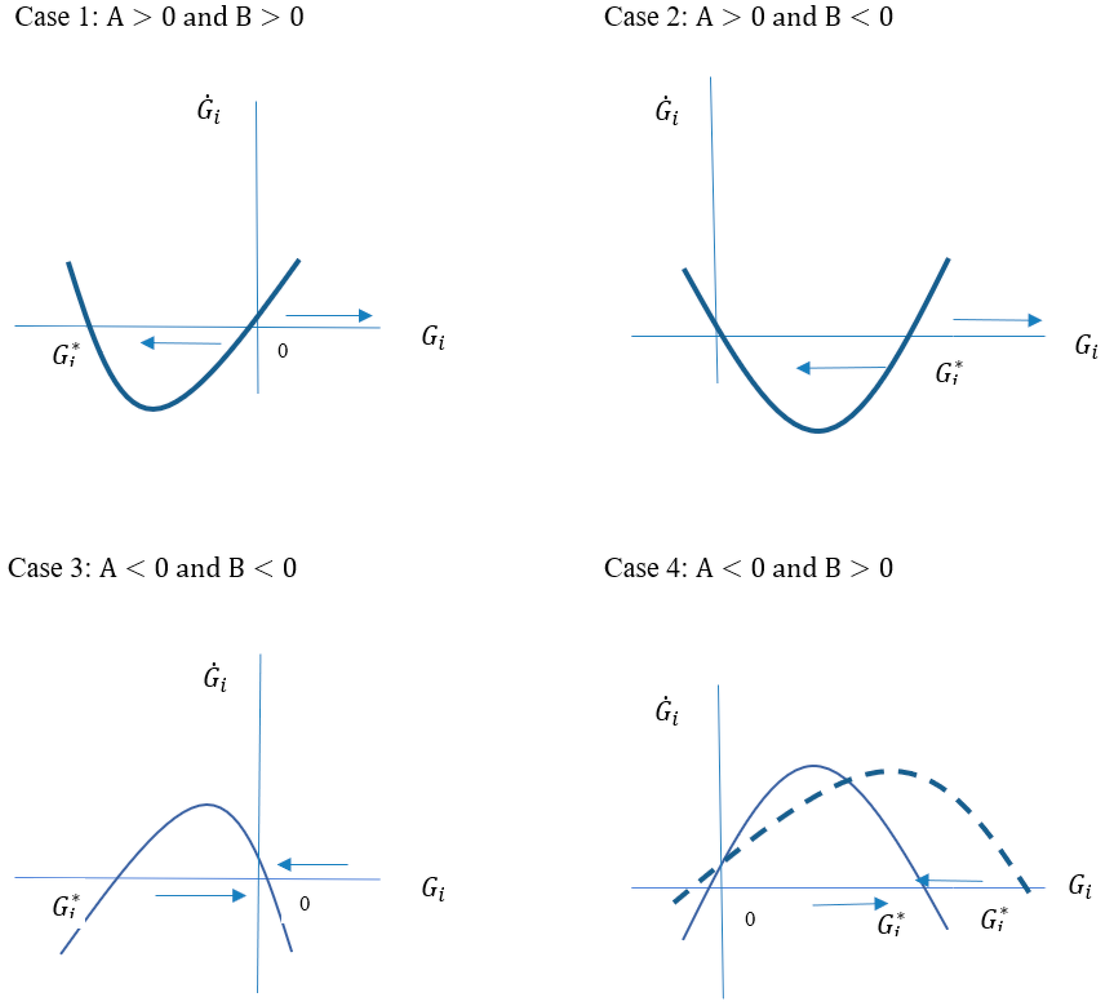
There are four possible cases depending on the values of
A and
B, and these are depicted in
Figure 1. In Case 1, the growth gap between the frontier and lagging country continues to increase (when the initial growth gap is to the right of the origin) or the lagging country catches up to the frontier country (when the initial growth gap is to the left of the origin). However, since the lagging country has a lower income level than the frontier country, it is not possible for the initial growth gap to be to the left of the origin. Thus, Case 1 necessitates that the growth gap between the frontier and lagging country continues to expand. In this case, A > 0 means that the negative effect of the growth gap (
) from a low enrollment ratio due to low economic development dominates the positive effects of the growth gap (
), such as knowledge and technology spillover effects. B > 0 means that the social capability, which is referred to by [
45], of the lagging country is lower than that of the frontier country. This is the case when the interest rate is higher in the lagging country than in the frontier country due to the lagging country’s undeveloped financial markets, and when the secondary education enrollment ratio in the lagging country is lower than the ratio in the frontier country. The positive or negative effects of income inequality in the lagging country are relatively low. In terms of income inequality, the positive effect of income inequality is dominant (i.e., in innovation and investment) in the frontier country, while its negative effect is dominant in the lagging country.
Case 2 shows a scenario with a certain threshold effect on the growth gap between the frontier and lagging countries. In other words, convergence between the frontier and lagging countries occurs when the initial growth gap is below a certain level (), but growth diverges when the initial growth gap is above . This occurs when, as in Case 1, the negative effect of the growth gap is larger than its positive effect. Unlike Case 1, however, the social capacity of the lagging country is higher than that of the frontier country in Case 2. Thus, Case 2 shows that for a lagging country with a relatively small growth gap with the frontier country, its high social capacity makes it possible to catch up to the frontier country. However, if the lagging country has a larger growth gap with the frontier country, it fails to catch up to the frontier country in spite of its high social capacity.
Case 3 is the opposite of Case 1 in that the advantages to the lagging country are stronger than the weaknesses (i.e., A < 0), and the social capacity of the lagging country is higher than that of the frontier country (B < 0). That is, the effect of technological diffusion from the frontier country is sufficient, and the lagging country has a lower interest rate, higher secondary enrollment ratio and higher effect of income inequality than that of the frontier country. In this case, the lagging country can catch up with the frontier country regardless of the initial growth gap.
In Case 4, the gap converges to an equilibrium. In this case, the advantages as a lagging country are stronger than the weaknesses, while the social capacity of the lagging country is lower than that of the frontier country. Facing such circumstances, the gap converges to the equilibrium gap of . However, if the social capacity of a lagging country is lower than the social capacity of other lagging countries, the equilibrium growth gap will increase from to . This can happen when the financial markets are not well developed, the interest rate is high, and/or the secondary enrollment ratio is low. An equilibrium gap also results if the level of income inequality is high when the negative effect of income inequality is dominant and/or the positive effect of income inequality is dominant when the level of income inequality is low.
4. Estimation Results
To see how the increase in income inequality affects the growth gap, a reduced Equation (12) was estimated for 43 countries in 1991–2014 and
Table 1 shows the These indicate that catching up during the investigated period was faster when the initial growth gap with the US (the frontier country) was greater. The estimation result of Model (1-1) corresponds to Case 4 of
Figure 1, where lagging countries fail to completely catch up with the frontier country (the US), and the gap converges to an equilibrium growth gap. Model (1-2) is the result of estimating Model (1-1) by adding the income inequality gap (
) between the frontier and lagging country. The results show that the growth gap between the frontier and lagging country increases as the income inequality of lagging country
i widens, implying that increased income inequality in country
has a negative effect on growth.
Table 2 shows the effect of income inequality on economic growth using a three-stage least squares estimation method (3SLS). The average growth rate of patents filed with the USPTO between 1991 and 2014 is used as a proxy to capture a country’s innovation capability. Instead of the rate of increase in capital stock, this estimation uses the investment ratio (
) as a proxy variable because of the technical difficulties involved in obtaining consistent values for capital stock due to differences in data collection methodologies between countries. If
is constant, the growth rate of capital stock (
) is proportional to the investment rate (
). For this reason, we use the investment rate as a proxy for the growth rate of capital. Lack of comparable data on inequality measures is one of the biggest challenges in studying income inequality between a large number of countries. For example, though there are many household surveys of distribution, these are often not comparable with each other. Direct comparison is impossible because some surveys measure income on a per-capita basis, while others measure income by household. Some surveys also measure disposable income, while others measure total spending. [
46] has divided such surveys into 21 categories and proposed a methodology for converting these into standard measures of net and market inequality. Under this proposal, Solt defines net inequality as a computed level of income inequality based on income after direct taxes and subsidies, while market inequality is the degree of income inequality derived from a pre-tax and pre-subsidy income basis. In our study, we use net equality, which represents the degree of income inequality after income redistribution and which is obtained from SWIID 6.2 constructed by Solt. The estimation results using Gini coefficients from the World Development Indicators, which are widely used in inequality-related studies, are provided in
Appendix A and these show similar results.
Unlike Model (1-1) in
Table 1, Model (2) in
Table 2 considers growth through various routes such as technology innovation, investment, human capital accumulation, and income inequality. Models (3) through (5) are estimated taking into account regional characteristics. Model (3) is a comparative analysis of the effects of income inequality on growth, dividing countries into developed and developing countries. There are 29 developed countries in our analysis: Australia, Austria, Belgium, Canada, Chile, Czech Republic, Denmark, Finland, France, Germany, Greece, Holland, Hungary, Iceland, Israel, Italy, Japan, Korea (South), Mexico, New Zealand, Norway, Portugal, Singapore, Slovakia, Spain, Sweden, Switzerland, the UK, and the US. Furthermore, 14 countries are categorized as developing countries, including Argentina, Brazil, China, Colombia, Egypt, India, Indonesia, Malaysia, Philippines, Russia, South Africa, Thailand, Turkey and Venezuela. We classify countries as developed (or high-income) if their GNI per capita is more than
$12,236 and developing if it is less than
$12,236 in 2016 according to the World Bank. Model (4) focuses on the characteristics of Asian countries and analyzes how the effects of income inequality on growth in Asia are different from those of other countries. On the other hand, Model (5) focuses on the characteristics of South American countries and compares the Latin American region with other countries. The regional dummy variables,
, are developed country, developing country, Asian country, and South American country dummies, respectively.
The first equation in Model (2) estimates the determinants of productivity and finds that over the past 25 years, investment in fixed capital has been the driving force of productivity growth. As suggested by [
34,
47, it can be seen that investment has contributed to productivity improvements by introducing new technologies embodied in equipment or machines and in learning by using. The results do not confirm, however, the contribution of technology innovation to productivity as measured by the number of patent applications. Second, the tertiary enrollment ratio, which represents a determinant of technological innovation, is positively affected and statistically significant. In line with [
35,
36], catch-up effects also showed a positive influence on technological innovation, implying that technology spillovers from the frontier country play a positive role in technological innovation. However, we were unable to achieve statistically significant results when checking whether income inequality has a positive or negative effect on technological innovation. The results do not confirm that income inequality drives innovation and entrepreneurship as suggested by [
1,
2,
15] and also do not demonstrate that income inequality has a negative impact on innovation as argued by [
8,
39,
40]. The third equation is an estimate of the investment function. The coefficient for the GDP growth rate is positive and statistically significant, confirming that the acceleration principle applies to investment. However, we cannot confirm that the real interest rate has a negative impact on investment. The impact of income inequality on investment is statistically significant with a negative sign, indicating that income inequality has a negative effect on investment. Unlike the predictions of [
10,
11], the results support the findings of [
23,
43]. This model assumes a cumulative relationship among productivity, growth, and investment; that is, a high rate of investment leads to productivity improvements, productivity improvements lead to growth and growth increases investment, thus creating a virtuous circle. Or conversely, a low rate of investment leads to low productivity, low productivity leads to low growth, and low growth is connected to low investment, thus forming a vicious circle among these factors. The results of this study confirm such a cumulative relationship among productivity, growth, and investment.
An estimation of human capital accumulation, the third path through which income inequality affects growth, was conducted in the fourth estimation equation. The higher education enrollment ratio, which represents the level of human capital, is positively influenced by the secondary enrollment ratio. Also, there exists a negative correlation between a higher education enrollment ratio and the level of economic development (
), indicating that the lower the level of economic development, the lower the enrollment rate of tertiary education. On the other hand, unlike studies by [
19,
20,
21], our study fails to confirm that income inequality has a negative effect on human capital accumulation.
Authors of [
10,
11] emphasize that, depending on the level of economic development, income inequality can positively affect growth. In other words, in developing countries where capital is insufficient compared to developed countries, the concentration of wealth in the rich with a high propensity to save will increase investment. To investigate this, Model (3) analyzes the effects of inequality on growth by dividing the sample into developed and developing countries. The estimation results are similar to Model (2); thus, we fail to find that inequality has an impact on technological innovation and human capital accumulation, which can affect a country’s economic growth, but we do find that unequal income distribution has a negative impact on investment in both developed and developing countries. In other words, unlike Kaldor and Barro’s predictions, we find that income inequality negatively affects investment even in developing countries. The coefficients of estimation are similar for both developed and developing economies, at −0.1577 for developed countries and −0.1691 for developing countries.
Models (4) and (5) show the estimation results obtained when controlling for regional characteristics. Model (4) includes the Asian region dummy in the estimation equation. It is notable that the effect of inequality on the investment function is relatively low compared to other regions. In Asia, the estimated coefficient of income inequality is −0.0289 (−0.1554 + 0.1265), but in non-Asian countries it is −0.1554. This indicates that the negative effects of income inequality on investment are relatively low in Asia. In addition, income inequality has a negative impact on human capital accumulation in Asian countries, although it is statistically significant only at the 10% level. In addition, as shown in the second estimation equation of Model (4), human capital has a positive effect at a 10% significance level on technological innovation as measured by patent applications, and this innovation has a positive effect on productivity improvements. In summary, income inequality in Asian countries has a negative impact on human capital accumulation, and this low human capital accumulation has a negative impact on technological innovation, and ultimately, low technological innovation has a negative impact on growth.
Model (5) includes the South American dummy. The path through which income inequality negatively affects growth in the South American region can be confirmed through the second and first equation. In the second equation, the coefficient of the term combining inequality and the South American dummy has a negative sign, which means that as South American income inequality increases, technological innovation decreases. Combined with the first estimate of productivity, we find that the increase in income inequality in South American countries has a negative impact on technological innovation, which in turn has a negative impact on productivity growth. In the end, both in Asia and Latin America, income inequality has a negative effect on technological innovation, which in turn has a negative impact on productivity improvement and growth. However, in Asian countries, inequality has a negative effect on technological innovation by influencing human capital accumulation, whereas in South American countries, income inequality has a direct negative effect on technological innovation.
5. Conclusions and Summary
Previous studies argue that income inequality has positive and/or negative effects on technological innovation, investment and human capital accumulation, and therefore, ultimately affects sustainable economic growth. Even though income inequality can have an impact on economic growth through various routes, previous studies have focused on the individual relationships between income inequality and technology innovation, between income inequality and investment, or between income inequality and human capital. Without comprehensively understanding how these factors interact with each other, it is not possible to systematically explain the effects of income inequality on sustainable economic growth. In this study, we examine how income inequality affects growth through three paths: technology innovation, investment, and human capital. Based on a cumulative growth model that includes all three paths, we empirically test the effects of income inequality on growth for 43 countries from 1991 to 2014. The results of the analysis are summarized as follows.
First, the estimation results using a reduced equation reveal that a positive correlation exists between the income inequalities of lagging countries and the respective growth gaps with the frontier country. This confirms that an increase in income inequality negatively affects growth.
Secondly, the estimation of a cumulative growth model using 3SLS estimation shows that income inequality has a negative effect only on investment. However, we fail to find correlations between technological innovation and income inequality and between human capital accumulation and income inequality. Considering that investment has a positive impact on productivity, we conclude that income inequality has a negative impact on investment and that the resulting sluggish investment has a negative impact on productivity, which in turn negatively influences growth.
Third, Kaldor and Barro argue that the effect of income inequality on growth differs depending on the level of a country’s economic development. Therefore, in this study, we used dummy variables that classify countries according to their economic development level. In contrast to Kaldor and Barro’s estimates, our results show that income inequality in developing countries has a negative impact on growth, particularly as it impacts investment. The effects of income inequality on investment are found to be similar in both developed and developing countries.
We also find that there are region-specific differences in how income inequality affects growth. In the case of Asian countries, income inequality is negatively associated with growth through two paths. First, income inequality is found to negatively impact investment, but this negative effect is relatively low compared to other regions. It is also noteworthy that income inequality in Asian countries has a negative impact on human capital. Reduced human capital has a negative impact on technological innovation, which ultimately has a negative effect on growth. In other words, we find that there exists a cause-and-effect chain from income inequality to human capital accumulation, on to technological innovation and finally to sustainable economic growth.
Lastly, income inequality in South American countries has a negative impact on technological innovation, which in turn has a negative impact on productivity and economic growth. Both Asian and Latin American countries show similarities in that income inequality has the same negative effect on technological innovation, which has a negative impact on productivity and growth. However, in Asian countries, income inequality negatively affects technological innovation by suppressing human capital accumulation, whereas in South America, income inequality directly affects technological innovation.
It is difficult to propose definitive policy implications due to the inherent limitations of cross-country regression analysis using incomplete datasets. However, our results suggest that government efforts to mitigate income inequality will accelerate investment, human capital accumulation and technological innovation, and that this can play a positive role in reducing the growth gap between countries and realizing sustainable economic growth.


