Real Time Implementation of Learning-Forgetting Models for Cycle Time Predictions of Manual Assembly Tasks after a Break

Abstract

Industry 4.0 provides a tremendous potential of data from the work floor. For manufacturing companies, these data can be very useful in order to support assembly operators. In literature, a lot of contributions can be found that present models to describe both the learning and forgetting effect of manual assembly operations. In this study, different existing models were compared in order to predict the cycle time after a break. As these models are not created for a real time prediction purpose, some adaptations are presented in order to improve the robustness and efficiency of the models. Results show that the MLFCM (modified learn-forget curve model) and the PID (power integration diffusion) model have the greatest potential. Further research will be performed to test both models and implement contextual factors. In addition, since these models only consider one fixed repetitive task, they don’t target mixed-model assembly operations. The learning and forgetting effect that executing each assembly task has on the other task executions differs based on the job similarity between tasks. Further research opportunities to implement this job similarity are listed.

1. Introduction

Since the raise of mass customization, manual assembly operators are indispensable for many manufacturing companies [1]. They provide the necessary flexibility to assembly lines which automated systems cannot. Nevertheless these operators need more support because of the high cognitive load that comes along. They are assumed to be capable of performing a broad range of tasks and they have to be able to do the right task at the right moment. Different on-the-job training strategies for supporting operators can be distinguished: providing (digital) work instructions, micro learning moments, expert based training, virtual training, etc. These techniques are highly helpful and can avoid unnecessary cycle time increase or variation and deficiencies on the product’s quality.

However, just supporting an operator with one or more of these tools is not sufficient. An operator who is well experienced does not need the same support as an operator who is new at the assembly line. This difference in experience should result in another method for supporting the operator. An operator-tailored support can be achieved, for example, by adapting work instructions [2] or by choosing an alternative form of support based on the current competence level of the operator. A major challenge for companies is to estimate this competence level of their operators and keep it up to date. The introduction of industry 4.0 provides manufacturers with a large amount of data. Different kinds of sensors are implemented in order to capture as much contextual information as possible. This sensor data can also indicate the workers’ competence level, which can be used for operator-tailored support.

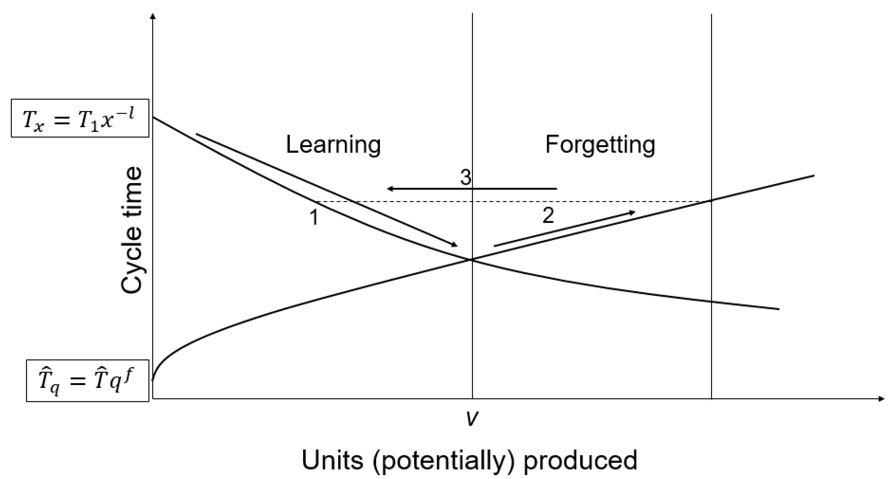
One of the most important indicators for operators’ experience is the production cycle time. In general, a decrease of the cycle time will occur during production. This so called learning effect was first described by Wright [3], but has been researched quite a lot [4]. In addition, different models are introduced to model this effect. The prediction of cycle times based on learning has many applications. One of the most found applications are optimization techniques for inventory cost [5], optimal batch sizes [6,7,8] and workforce management [9,10]. These applications need a long term prediction. This is different for the estimation of a worker’s experience level. There is a need for real time data to initiate operator tailored support. A lot of systems are already used for automatically registering cycle times of operators [11]. With the aid of these data, the transition of an operator from one level to another can be monitored.

Next to this effect of learning, operators start to forget when they don’t perform their task for a while [12]. During this break, the cycle time will virtually start to increase again. Different mathematical models were presented in the last decades [13,14,15]. In most of the models, the first cycle time for the next production iteration depends on the length of the break and the experience gained at the beginning of the break. Next to this factor, different other factors are taken into account, depending on the model. The cycle time of an operator during a break cannot be registered by any system. Thus, an estimation of the workers’ experience level during a break must be made. The models that are presented in literature can be used for this purpose.

All learning forgetting models that are found in literature are used for a long term planning. In this paper we compare the real time implementation of different learning forgetting models. Different modifications are suggested in order to optimize the models and to make them more robust.

The purpose of the real time cycle time prediction is to have a clear view on the operator’s experience level at all time. Different operator support tools can use this as an indicator to provide operator-tailored information. Both the amount of information and the level of detail can be adjusted to the operator’s needs, which improves the quality and productivity of the worker [16]. The cycle time prediction as a measure of experience level can also be used for quick, short term job rotations, due to the absence of an operator. In addition, a higher cycle time can indicate quality issues [17]. When a new production cycle starts, there is no baseline yet for comparing the actual assembly time with. The estimation of the cycle time after a break can be used as such and quality issues can be tracked more accurately.

In Section 2, a brief overview of the most commonly used learning forgetting models is given. The models that are used for real time implementation are discussed in detail. Since the models that are found in literature are not dynamic enough for real time predictions, some adaptations for each of the models were developed and presented in Section 3. This section focusses on the assumptions and modifications that were made to make the model useful and logical. Real time cycle time registrations and the duration of a break are the input for the further developed models. The models were validated on empirical data. The results and discussion can be found in Section 4. At last, the conclusion of this study and future research perspectives are stated in Section 5.

2. Learning and Forgetting Models

The aim of this study is to find a way of predicting the cycle time of a manual assembly operator after an interruption of production. In order to do so, different learning and forgetting models were studied. Since the forgetting effect is strongly correlated to the learning rate of an operator [18], these developed models are of great interest in this study. In literature, many different models were introduced for the prediction of cycle times of manual assembly tasks based on the learning and forgetting effect. Predictions are made for both production periods where learning occurs and interruptions where a decrease of experience is expected. In this section we give an overview of the most commonly used models. Many comparative studies of learning forgetting models can be found [19,20]. In this study we made a selection of the models that showed the best performance on fitting data in these earlier contributions. These are also the models that are most recently cited.

2.1. Learn–Forget Curve Model (LFCM)

The learn-forget curve model was introduced by Jaber and Bonney [13] and differs from earlier models by including the total forgetting time. They state that the forgetting rate depends on the learning rate, the minimum production break over which total forgetting occurs and the amount of accumulated experience that the operator has at the beginning of a break.

As many other models they use the learning curve of Wright (WLC) [3] which is given by the following equation:

$$T_x=T_1{x}^{-l},$$

(1)

where T_x represents the cycle time for the xth assembly iteration and l represents the learning slope. T₁ is the cycle time of the first assembly iteration. The learning curve is assumed to be fixed for each specific operator-task combination. After an interruption, the same function will be followed. The starting point of the next production cycle depends on the forgetting period. The forgetting effect is modeled with a similar power function:

$${\widehat{T}}_q={\widehat{T}}_1{q}^f,$$

(2)

Similarly to the learning curve, ${\widehat{T}}_q$ represents the cycle time of qth unit of lost experience on the forgetting curve. The amount q is the output that would have been produced if no interruption had happened. ${\widehat{T}}_1$ is the equivalent of T₁ and equals ${\widehat{T}}_q$ when q equals 1. The learning slope is given by f.

This is very similar to the Variable Regression to Invariant Forgetting (VRIF) model [21] and the Variable Regression Variable Forgetting (VRVF) model [22]. The way these models differ from each other is the interpretation of the forgetting curve. The VRIF makes use of a fixed forgetting slope and ${\widehat{T}}_1$. This means that the forgetting curve does not change in time. The VRVF adapted the VRIF by using a variable ${\widehat{T}}_1$. As the forgetting slope is still fixed, the ${\widehat{T}}_1$ is calculated so it intercepted the learning curve at the point a break starts. Different studies concluded that the forgetting rate depends on the learning rate [23]. Although there is not a full consensus on this topic, most of the studies indicate that a higher learning rate results in a higher forgetting rate [24]. This finding was implemented in the LFCM.

To calculate the forgetting slope of the ith production-break cycle f_i, the following equation is presented:

$$f_i=\frac{l\left(1-l\right)\ast \log \left(v_i\right)}{\log \left(\frac{t_B}{t\left(v_i\right)}+1\right)},$$

(3)

where v_i is the amount of cumulative experience that was gained at the end of the production cycle i. The time to produce an output of v_i is given by $t\left(v_i\right)$ and the total forgetting time is represented by t_B. The total forgetting time is a fixed parameter which depends on the job and should be derived empirically. Figure 1 shows the first learning-forgetting cycle with the LFCM. Every cycle, the forgetting slope changes depending on the gained experience before the break.

2.2. Recency Model

The Recency model (RC) [14] was compared by Nembhard and Osothsilp [19] to 13 other models and was found to be the best to fit to an empirical dataset. This model uses the WLC as well and depending on the recency of the experience, the model will predict the cycle time after a break following:

$$T_x=T_1{(R_x^{\alpha }x)}^{-l},$$

(4)

with

$$R_x^{}=2\frac{{{\displaystyle \sum }}_{i=1}^x(t_i-t_0)}{x\left(t_x-t_0\right)}$$

(5)

R_x is the recency of experimental learning. In this equation x is the cumulative output at time t_x and α is a fitting parameter. The timestamp of finishing the ith assembly iteration is given by t_i. The parameter α indicates how easily an operator forgets his tasks and is thus an individual property. If α tends to equal 0, this means that the operator does not forget his tasks. This model does not take into account the length of the breaks and is mainly used to check irregular production breaks. In this study we focus on long production breaks in comparison with the cycle time.

2.3. Power Integration Diffusion

Sikström and Jaber [15] indicated some limitations of the RC model and presented the Power Integration Diffusion (PID) model. The RC model is not in compliance with Jost’s law that states that newer memory decays faster than old memory [26]. The basic principle of this model is that every task completion forms a memory trace. The strength of the memory trace decays as a power function over time. Multiple repetitions will aggregate to a single stronger memory trace. The equation for predicting the next cycle time T_x at timestamp t_r is:

$$T_x=\frac{S_0^{\prime }}{{{\displaystyle \sum }}_{i=1}^N {{(t_r-t_{i.1})}^a}^{\prime }-{{(t_r-t_{i.2})}^a}^{\prime }}+t_0,$$

(6)

In this equation, i indicates the production-break cycle, $t_{i.1}$ refers to the start time of the ith cycle and $t_{i.2}$ to the timestamp of the end of this cycle. The parameter t₀ is fixed and equals the time to produce a single product while the operator is fully trained. The relationship of ${S^{\prime }}_0$ and a’ with the WLC is given by:

$${\mathrm{a}}^{\prime }=\frac{l}{1-\mathrm{l}}$$

(7)

and

$${S^{\prime }}_0=\frac{T_1^{\left(1+a^{\prime }\right)}}{\left(1+a^{\prime }\right)}.$$

(8)

3. Real Time Implementation

Since the discussed models of Section 2 showed the best results in matter of matching empirical data, it can be stated that they have great potential to be used for the prediction of cycle times after a break.

In this section we describe how the implementation of the aforementioned models was done in order to predict the cycle times of an operator after a break with the aid of real time cycle time registration. The different models were already fitted to empirical data in different other studies to check how well they can approximate a real scenario of learning and forgetting. In this study, we don’t aim to find the best value for the parameters of each model to fit the empirical data the best, but we try to find which model gives the best prediction based on real time data.

The point of view here is that no parameters should be assigned anymore for the prediction, despite that the parameters in the different models are essential for the outcome. The optimal value for these parameters is different for every task and every person. The industrial relevance of using the models for cycle time prediction would decrease a lot if a method engineer would be responsible to find a decent value for these parameters for every operator-task combination. A self-learning system is thus required and is the focus of the presented adaptations to the existing models. In the next sections, a description of how these models were made more dynamic is given.

3.1. Learn-Forget Curve Model

Given the cycle times of the first production cycle, a WLC can be composed by using a regression method. The parameters T₁ and l are then known. After the first production cycle, the cumulative experience that was gained is just the amount that was produced during the first cycle time. The break length is considered known and the total forgetting time is a parameter that must be set at the beginning. The forgetting slope is then calculated by Equation (3). ${\widehat{T}}_1$ can be calculated by

$${\widehat{T}}_1={\mathrm{T}}_1{v}^{-\left(l+f\right)}.$$

(9)

To fulfil Equation (2), the amount that would have been produced if no break occurred (q) must be calculated. This was done by:

$$q={\left[\frac{t_{BREAK}\left(1-l\right)}{T_1}+{\left(v-0.5\right)}^{\left(1-l\right)}\right]}^{\frac{1}{\left(1-l\right)}}-0.5,$$

(10)

This differs slightly to what is presented in earlier work but is a little more accurate. After the prediction of the cycle time after the break, a new production cycle takes place and the cumulative experience gained will change. The equivalent of the cumulative experience gained at the beginning of this cycle is the according value of x in Equation (1) for the predicted time. Every production iteration during this production cycle will increment the cumulative experience by 1.

The prediction of the cycle time after a break cannot exceed the value of T₁. If the prediction is higher than T₁, total forgetting occurred and the given prediction equals logically T₁.

The above described implementation of the LFCM has some disadvantages. Firstly, the parameter t_B is a fixed value and will very likely differ for every operator. Secondly, the parameters of the WLC are fixed during the whole process. If there are not a lot of assembly iterations during the first productions cycle, the estimation of the worker’s LC will not be accurate. Therefore, an adaptation of this implementation is suggested in order to counter these two drawbacks.

To avoid the dependency on a well-chosen total forgetting time, the modified LFCM (MLFCM) that was presented by Jaber and Kher [27] could be used. In this model the total forgetting time changes depending on the experience that was gained at the beginning of the break. They showed that the forgetting curve could be approximated by a linear function between the end of the production period and the timestamp where T₁ is reached. The model also assumes that for one time unit ($\Delta d$) during forgetting, a certain fixed amount of units (j) experience is lost. Subsequently, the total forgetting time is calculated by:

$$t_B=\frac{T_1-\left(T_1{v}^{-l}\right)}{\frac{\left(T_1{\left(v-j\right)}^{-l}\right)-\left(T_1{v}^{-l}\right)}{\Delta d}}.$$

(11)

This model provides a variable total forgetting time but still depends on the parameter j. The optimal value for j is hard to predict or estimate. However, the optimal value for j can be calculated after each break with the real first cycle time of the next production period. By performing this reverse calculation, an estimation of j is found for the next prediction.

At this point one uncertainty of the initial LFCM is countered, using an existing model. The second dependency of the model are the cycle times of the first production period. In reality, the operator’s cycle times will never exactly follow the WLC and moreover the first production period often has a lot of variation considering completion times due to a large amount of uncertainties [28]. The next step is to use the registered cycle times during all production cycles for adapting the WLC during the process. The equivalent of the cumulative experience gained at the beginning of this cycle is the according value of x in Equation (1) for the predicted time. This value for x, together with the real first task completion time will be added to the data points for the regression. In the same way, a data point for all assembly iterations is added and a new WLC will be obtained.

In order to avoid an instable system, only data points with a relatively small value for x are added in the implementation. The reason for this filtering is that an operator with a high accumulated experience will arrive at a steady state situation. Theoretically, the improvement in this situation will be very little, while the real situation will give quite some variance. This variance will affect the regression too much since the steady state situation is not included in the WLC. The accumulated experience at steady state is hard to predict and depends on the operator and the nature of the task. As a simplification for this model, we have chosen to use this point when a next assembly iteration causes a smaller improvement than 5% of the improvement between the first and second assembly iteration.

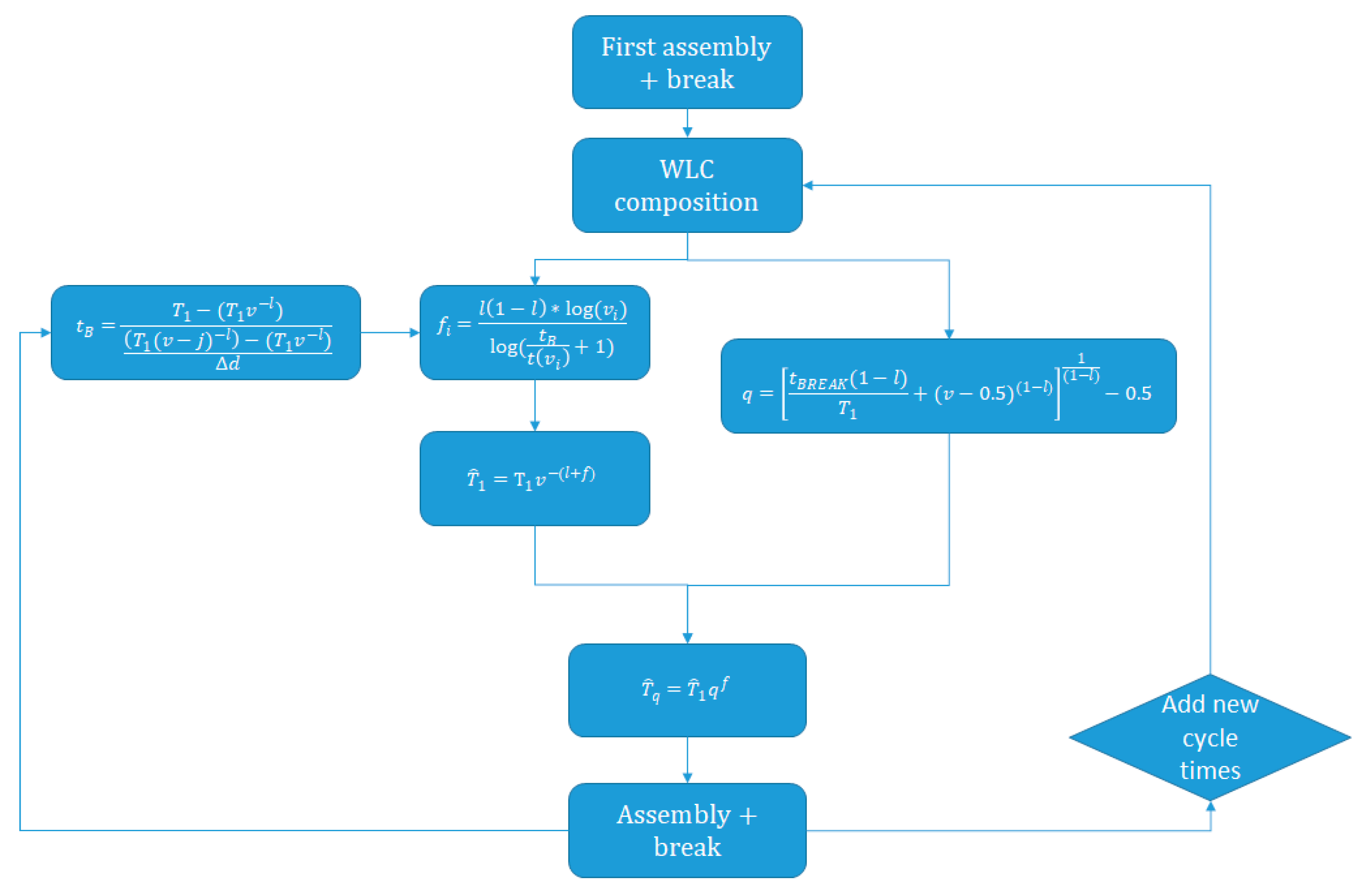
Furthermore after each production-break cycle, half of the data points are deleted. Only the data points that fit the best on the current WLC are kept. This will avoid outliers to influence the system during a longer period and will reduce the computational effort. The approach is presented in Figure 2. This model will be further addressed as the adaptive MLFCM.

3.2. Recency Model

The recency model has only one parameter on which the prediction of the cycle time after a break depends, namely α. Similarly as with the implementation of the LFCM, it is possible to calculate the optimal value for α for each production break cycle after the first assembly of each production period.

Two different implementations were tested. The first one is using the previous optimal value for α for the next prediction. The second method uses the average of all previous cycles to estimate the cycle time of the assembly task after a break. The calculation for the optimal value of α was done by:

$${\alpha }_{Optimal}=\frac{\log \left(\frac{{\left(\frac{T_{i,1}}{T_1}\right)}^{-\frac{1}{l}}}{x}\right)}{\log \left(R_x\right)}$$

(12)

and limited between 0 and 10, in order to avoid overshoot. $T_{i,1}$ represents the first cycle time of the next production period, the value of R_x is the value that was used for the previous prediction and is calculated by Equation (5).

3.3. Power Integration Diffusion

For the implementation of the PID model, the parameter t₀ must be assigned a value. It is proposed that the parameter will change over the cycles based on the deviation between the prediction and the real cycle time. For the first cycle, half of T₁ was chosen. After the first cycle, t₀ will be calculated by:

$$t_{0,i}=t_{0,i-1}+\left(T_{i,1}-T_{pred}\right).$$

(13)

Equations (7) and (8) were used to find a’ and S′₀. The values of the WLC were derived from the first production period.

4. Results and Discussion

The models, described in Section 3, were used to predict cycle times after a break for different subjects and for multiple learn-forget cycles. In this section the results of the predictions for each model will be presented and compared.

All implementations are tested on a dataset that consists of learn-forget cycles of 5 operators in a real production setting of the assembly of a backbone for a children’s car-safety seat. The amount of repetitions for each production period varies from 3 to 59. The amount of learn-forget cycles varies from 9 to 18 and the break times differ from 1 to 146 h. Breaks shorter than 1 h are not taken into account for the prediction models. The subjects never had to assemble for more than one and a half hours consecutively. This avoids the influence of fatigue that could affect the subjects’ concentration. The workstation was separated from the rest of the production hall in order to avoid environmental influences and subjects’ distractions.

All assembly completion times were registered with the aid of the Human Interface Mate (HIM^®) of Arkite. This is a digital operator support system that registers the completion of all assembly steps via a 3D sensor. During the assembly, the HIM^® also provides the operator with instructions that are showed by vertical projection on the workstation. While following up the process, all timestamps of the transitions of one assembly step to the next are logged. An overview of the amount of assembly iterations and break lengths (in hours) for all learn-forget cycles is given in

Table 1. Amount of assembly iterations and break lengths for each learn-forget cycle.

Cycle	Operator A	Operator B	Operator C	Operator D	Operator E
Assembly Iterations (Break Length in Hours)
1	8 (19)	15 (22)	13 (43)	4 (26)	12 (76)
2	13 (23)	19 (23)	17 (21)	6 (44)	20 (95)
3	17 (3)	17 (23)	16 (73)	6 (164)	22 (47)
4	18 (21)	18 (21)	16 (4)	3 (23)	26 (23)
5	21 (1)	15 (19)	17 (23)	6 (146)	25 (69)
6	19 (19)	15 (6)	15 (21)	4 (21)	25 (25)
7	20 (2)	17 (23)	20 (25)	7 (74)	29 (47)
8	21 (20)	15 (23)	18 (17)	6 (23)	25 (23)
9	21 (2)	17 (26)	19 (119)	8 (44)	27 (71)
10	23 (2)	17 (18)		4 (23)	27 (20)
11	23 (25)	54 (25)		7 (75)
12	23 (2)	29 (22)		10 (20)
13	20 (24)	57 (23)
14	22 (18)	50 (19)
15		55 (2)
16		3 (19)
17		49 (20)
18		27 (30)

.

The completion times were used as input for the different real time learning forgetting models. The performance of every model for every operator is presented in

Table 2. Mean relative error for each implementation per operator.

		Operator A	Operator B	Operator C	Operator D	Operator E	Total
WLC	T1	809	278	462	1331	338
	l	0.5000	0.0581	0.2417	0.5000	0.0892
LFCM	10	63.3%	37.0%	63.8%	57.6%	81.0%	57.1%
	100	35.6%	32.3%	39.8%	30.0%	74.8%	40.2%
	1000	21.4%	29.7%	26.7%	20.0%	62.7%	30.8%
	10,000	15.8%	28.0%	20.7%	16.4%	56.2%	26.5%
MLFCM	Normal	16.9%	27.9%	17.1%	12.3%	67.2%	27.8%
	Adaptive	6.09%	25.9%	16.7%	7.51%	7.55%	14.2%
RC	Normal	19.7%	28.5%	36.8%	14.9%	11.7%	22.8%
	Average	19.7%	31.5%	34.0%	17.0%	10.7%	23.5%
PID		5.98%	17.2%	18.8%	5.29%	11.5%	12.1%

. Due to a large variation of operator’s learning rate, the mean errors for the predictions are given relatively to the range in which the cycle time should be theoretically. We assume that forgetting always occurs during a break and that the cycle time will never exceed the value of T₁. Subsequently, the range is given by the difference between the fastest assembly iteration before the break and T₁. The relative error is the ratio of the absolute deviation to the described range. For the analysis, the predictions of the breaks where the first cycle time of a production cycle was shorter than the fastest cycle time of the previous cycle (improvement during a break), were excluded for the calculation of the mean relative error. This was only the case for two production cycles of operator D. The second iteration of this operator after those cycles were significantly longer. We assume that those two values were not well registered by the tracking system.

In every implementation of the different methods, a parameter changes every cycle, based on the previous error. Therefore, an alternating signal was expected in these graphs. In general, the models react on errors in the same way, but the proportion in which a previous error causes an effect on the next prediction differs. The implementation of the RC model seems to be less sensitive to the change of prediction errors. This might be the reason why the RC model shows a worse mean relative error overall. Furthermore there seems to be a tracking error for the RC model that is not covered by the presented implementation. The reason for this tracking error is probably that only the first production cycle is used for the determination of T₁ and l. However, although the PID model copes with the same problem, it shows much better results than the RC model.

The results indicate that a larger total forgetting time gives a better estimation of the production. As for this particular case, 10,000 days is the best chosen value. This is a very large value and doesn’t seem a realistic value for total forgetting. This confirms that it is very hard to estimate a good value for this parameter of the LFCM in order to do real time calculations. The MLFCM without adaptive WLC performs similarly to the LFCM with a total forgetting time of 10,000. This indicates that no parameter should be given upfront and that the method making use of equation 10 predicts the cycle time after a break equally well as making use of a well estimated value of the total forgetting time.

The MLFCM with adaptive WLC outperforms the model without variable WLC. The rules that were proposed in matters of stability seem to work and improve the original method significantly. Regarding the RC models, there is not a lot of difference between the two suggested implementations. Both are performing similarly. The models do not show the best predictions, nor the worst. The PID model gives the best results overall but there is only a little difference with the adaptive MLFCM and RC model.

For further comparison, only the adaptive MLFCM, the normal RC model and the PID model are taken into account because those methods show the best results. In Figure 3 the absolute errors for the predictions of all cycle times are represented for the three aforementioned methods. It is clear that the absolute errors oscillate along the x-axis. This indicates that the model adjusts the next prediction based on the error it made in the previous prediction. Only the RC model has a tracking error. This is mainly visual in the graphs of operators A, C and D. The RC model tends to perform better when the learning rate of the operator is higher.

The three methods that are outperforming the rest on first sight were compared to each other through a paired sample t-test. The results of the test state that the RC model gives statistically worse predictions in comparison with both the PID model (p < 0.001). For the comparison between the RC model and the adaptive MLFCM, the Pitman-Morgan test was performed because the variances are significantly correlated (p < 0.001). The test gives a t-value of 2.1872 and is higher than the critical value of 2.007 (df = 52; α = 0.975). This means that the adaptive MLFCM statistically significantly outperforms the RC model. The difference between the adaptive MLFCM and the PID model on the other hand is not statistically significant. 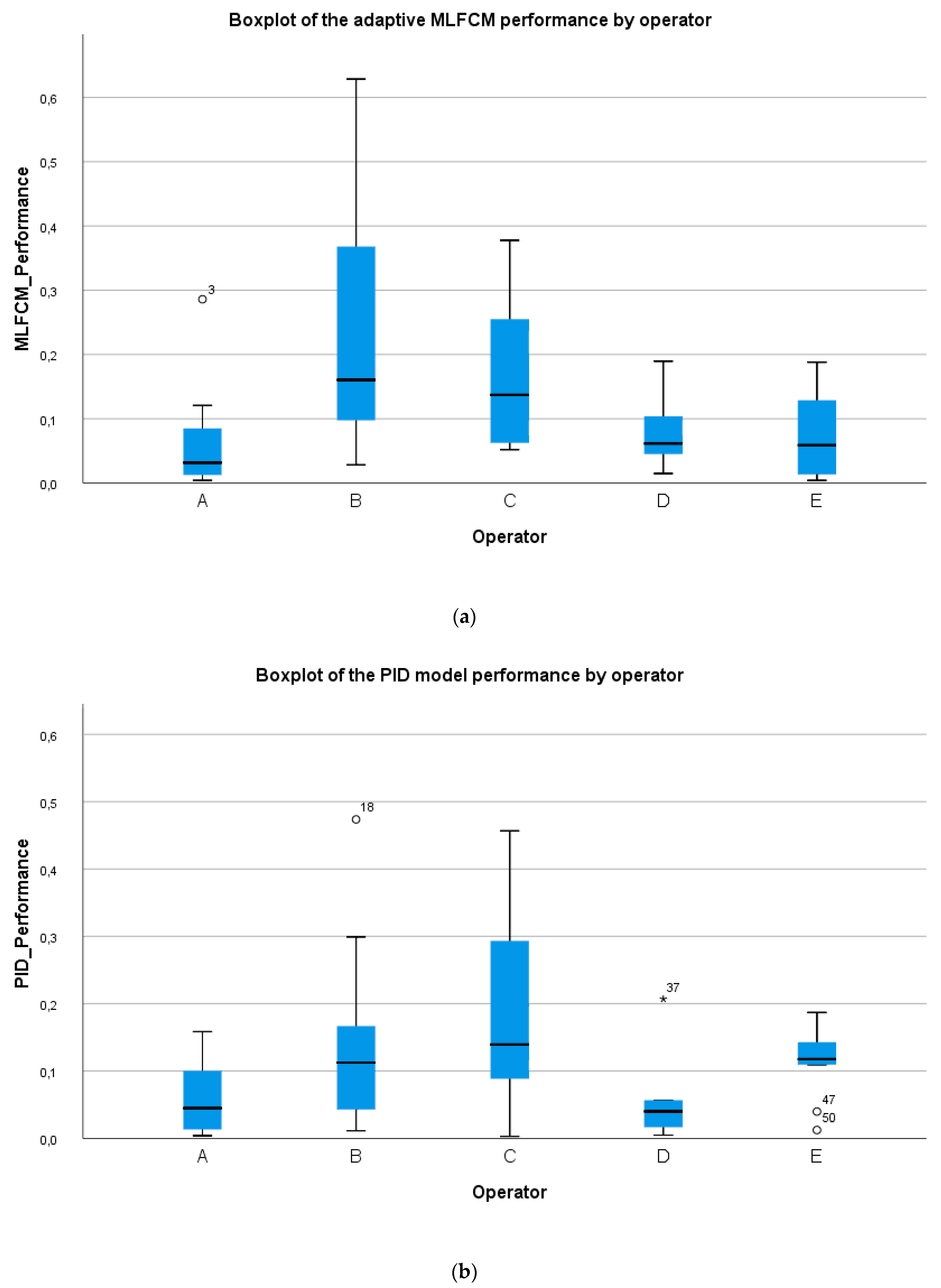Since the results show a correlation (p = 0.005), the Pitman-Morgan test was conducted as well. The according t-value is 0.7680 which is lower than the critical t-value 2.007 (df = 52; α = 0.975). In other words, none of those two models outperforms the other. The performance of both models are plotted and visualized in Figure 4. The outliers are defined by the Tukey’s hinges boundaries. The three cases (data points 3; 18; 37) of the high outliers are worth looking into detail to because they can give an indication of a further improvement.

The analysis of these three cases showed that the higher error is caused by the fact that the operator started to forget significantly slower than during the interruption(s) before. The production cycle before these cases show already a lower learning rate, but it is not sufficient for the model to adjust properly. The models immediately performed much better after this dissimilar forgetting effect due to their dynamic character. The dynamics of the models should thus still be increased to improve the overall performance. The model should anticipate this phenomena.

As for the adaptive MLFCM, a possible solution could be that more recently registered cycle times have a higher impact on the regression analysis to obtain the WLC. In the PID model, newer memory traces decay faster than old ones. The degree in which memory is kept could be implemented as a factor. This factor should be proportional to the rate of improvement.

Although these models show good results in this study, some improvements and extensions are still possible. The model only adjusts based on the latest prediction error and a selection of historical registered assembly iterations. Since all historical cycle times are available, an optimization of the models is possible. Different recurring situations could be detected and analyzed to improve the prediction model. In this way the outliers could be avoided. In addition, more contextual factors such as the temperature, current overall workload, etc. could be taken into account to achieve better results.

5. Conclusions and Future Perspectives

Different learning and forgetting models were evaluated for the use of cycle time prediction of manual assembly tasks. The models that were evaluated are: the LFCM, MLFCM, RC and PID model. Since these models are static and based on parameters, they are not fit to predict the forgetting effect after a break in real time. Therefore, some adaptations for each model are presented in order to improve the adjustability. The main change of the novel implementations is that the real time registered cycle times of an operator are taken into account. Based on this input, the adapted models counteract to possible tracking errors. In this way the models do not depend on any parameter and learns from earlier production-break cycles.

The models were tested on performance data of 5 operators. The subjects had to alternate assembly periods with periods of rest. The rest periods were varying from 1 h to approximately a week. During the rest period, subjects didn’t perform any task that is related to the task that was being performed during the experiment. The MLFCM and PID model show significantly better results than the other models.

However, some limitations of this study should be talked in future research. In this study, contextual factors were not taken into account and an isolated workstation was used to obtain the empirical data. A noisy environment could affect the knowledge transfer for example. Normally, slow learners forget slow as well, but in this case the environmental factors could change this general rule.

The second thing that should be handled is that there are sometimes suddenly bad predictions, after which the following predictions are much better. The models should be able to anticipate the bad predictions. Based on the results in this study, it can be stated that poor predictions are often caused by the fact that the operator seems to have reached a certain level of experience. S/he does not improve that much anymore during the assembly periods, and forgets much less than what the model expects. The slower improvement should be tracked more rapidly by increasing the impact of the registered experience gain of the operator. This might also result in a more dynamic system that is instable. Subsequently, additional rules to guarantee the stability should be added as well.

An alternative but potential solution to predict the cycle time after a break is the application of machine learning. However, this requires a lot of contextual data and historical data which is often not available.

Furthermore we aim to make at least one model operational for mixed-model assembly environments. In this study, there was just one fixed task to perform. In many cases, different models are assembled at the same production line (mass customization). Assembling one model can cause a learning or forgetting effect on others. The influence of job similarity on the forgetting effect was already shown in previous work [23]. Based on the work plan of an operator, his/her competence level could be estimated for all tasks in the near future. This can be used for identifying a lack of competence for any task. Subsequently, an additional operator supporting strategy can be applied, such as providing additional work instructions, scheduling a training, etc.