This study proposes a model that aims to improve the accuracy of the recommendation system by calculating review sentiment scores and integrating them with user ratings. In more detail, a domain-specific sentiment dictionary is constructed to derive the sentiment scores of user reviews. Then, based on the dictionary, the sentiment scores of the user review data are calculated and reflected in the recommendation system.
3.3. Step 3, Rating-Normalization
The user rating data are generally unequally distributed according to the user preferences. Owing to different criteria for rating items, there are users who generally tend to provide higher ratings, whereas other users tend to provide lower ratings. In the former case, a rating of 5 points would indicate a non-interesting movie, whereas this rating could indicate an interesting movie in the latter case. Hence, viewing the same rating scores of two different people in the same perspective cannot reflect the different rating tendencies and criteria of each person, as it could lead to a poor prediction accuracy. To reduce any bias caused from external factors, the data were normalized based on the personal evaluation tendencies of the users given that normalization can provide more accurate user similarities and user movie preferences.
In this study, we attempted to normalize user ratings by reflecting the rating tendency of users based on the differences in their preference for various items.
3.3.1. Movie Recommendation Approach Applying Differences in User Preferences or Partiality for Items
Based on user rating information, the difference or variances average rating score between items is calculated and then using it, the target user’s rating of a new item is predicted.
To calculate the differences in the preference for items, the average rating differences among the items are derived based on the item rating scores given by the users. The average user’s preference difference
between two items
i and
j can be derived by using Equation (1).
In Equation (1), the terms the rating difference of two items based on the users’ evaluations are expressed as , as .
The preference prediction can be derived from Equation (2), which uses the average rating difference obtained from Equation (1) to derive the rating
given by user
u for the new item
i.
Using Equation (2), the rating that will be given by user
u for the new item
i is predicted based on the rating for item
j. This can be achieved by adding the average preference difference
between items
i and
j to user u’s rating preference
for the rated item
j. Subsequently, the predicted values obtained using item
j are averaged to obtain
. This corresponds to the case where the importance for each predicted value is considered as a constant value of 1.
The number of users that evaluated both items i and j, , can be considered as the weight of item j, which can then be multiplied with Equation (2) to derive the relative importance of each item j. Equation (3) denotes the equation corresponding to the application of a weighted average.
3.3.2. Recommendation Method Applying User Rating Tendency
The accuracy of rating prediction is improved by reflecting user tendencies for determinations when rating with the recommendation method and applying the user preference differences to items.
The manner in which users decide the rating for a given item varies depending on the personal preference of each user. For example, in the case of movie ratings, when there are two users u1 and u2 who judge the rating based on the five different criteria of storyline, characters, story development, entertainment value, and cinematography, user u1 may rate a movie as 10 out of 10 as long as the movie satisfies the entertainment value criterion, regardless of other criteria. In contrast, user u2 may rate the movie as 6 out of 10 if any one of the five criteria are not satisfied. As such, the rating tendencies differ for each user depending on the user’s preference; therefore, a process for converting subjective data into more objective data is required to apply the rating data obtained from various users to predict a different user’s rating for a new item. Accordingly, if the collected rating data can be appropriately normalized based on users’ rating tendencies, a more accurate recommendation can be provided to a new user, u3. User rating normalization is the process of adjusting the data distribution of user ratings such that the entire sample data has the same median, and it is performed as follows.
1. Normalization based on a median of 5.5
Since the median rating score is 5.5 when the users can rate items on a scale of 1 to 10, the normalization is conducted based on the median value of 5.5 in order to adjust each user rating dataset distribution to have a minimum rating score of 1 and a maximum rating score of 10. For example, in the case where the maximum rating score given by user u1 is 8.0 out of 10, the process of normalizing a rating score of 7.0 given by user u1 is as follows. Since the score of 7.0 is greater than the median value of 5.5, the score is normalized by employing to adjust the score such that it lies within the common scale of 1 to 10. The normalization of the user’s rating score considering the minimum rating score is conducted similarly. For example, when the minimum rating score given by a user is 2.0, the user’s rating score of 3.0 can be normalized by adjusting the score to the common scale using .
2. Normalization of Data Between Median and Minimum in the Rating Value Range
When the range of a user’s rating data is within the range constituted by the minimum value and median value of the common scale only, the maximum value of the user rating is set as the median value of the common rating scale, 5.5. Additionally, the minimum value of the user rating is set as the minimum value of the common rating scale, 1. Subsequently, normalization is conducted based on the median value of this user rating range, which is 3.25.
3. Normalization of Data Between Median and Maximum Rating Value Range
Similar to the case described in 2, when the range of a user’s rating data is localized such that it lies between the maximum and median rating values of the common scale only, the maximum value of the user rating is set as the maximum value of the common rating scale. Additionally, the minimum value of the user rating is set as the median value of the common rating scale, and normalization is performed based on the median value of this user rating range, which is 7.75.
Based on the recommendation method that uses the user preference differences among various items, user rating normalization is applied according to the rating decision tendencies of users. The normalized rating data are applied to Equation (1). Through Equation (1), by using the rating data of users who rated both items i and j, the user rating differences for items i and j are aggregated. During this process, the rating data that have been normalized according to the individual user rating tendency for items i and j can serve as a more objective index in predicting the target user’s rating.
After normalizing the selected user rating data, the extracted normalized rating data from the users were transformed into a user x item rating matrix, with user, item, and rating relations, as shown in
Table 1 [
25].
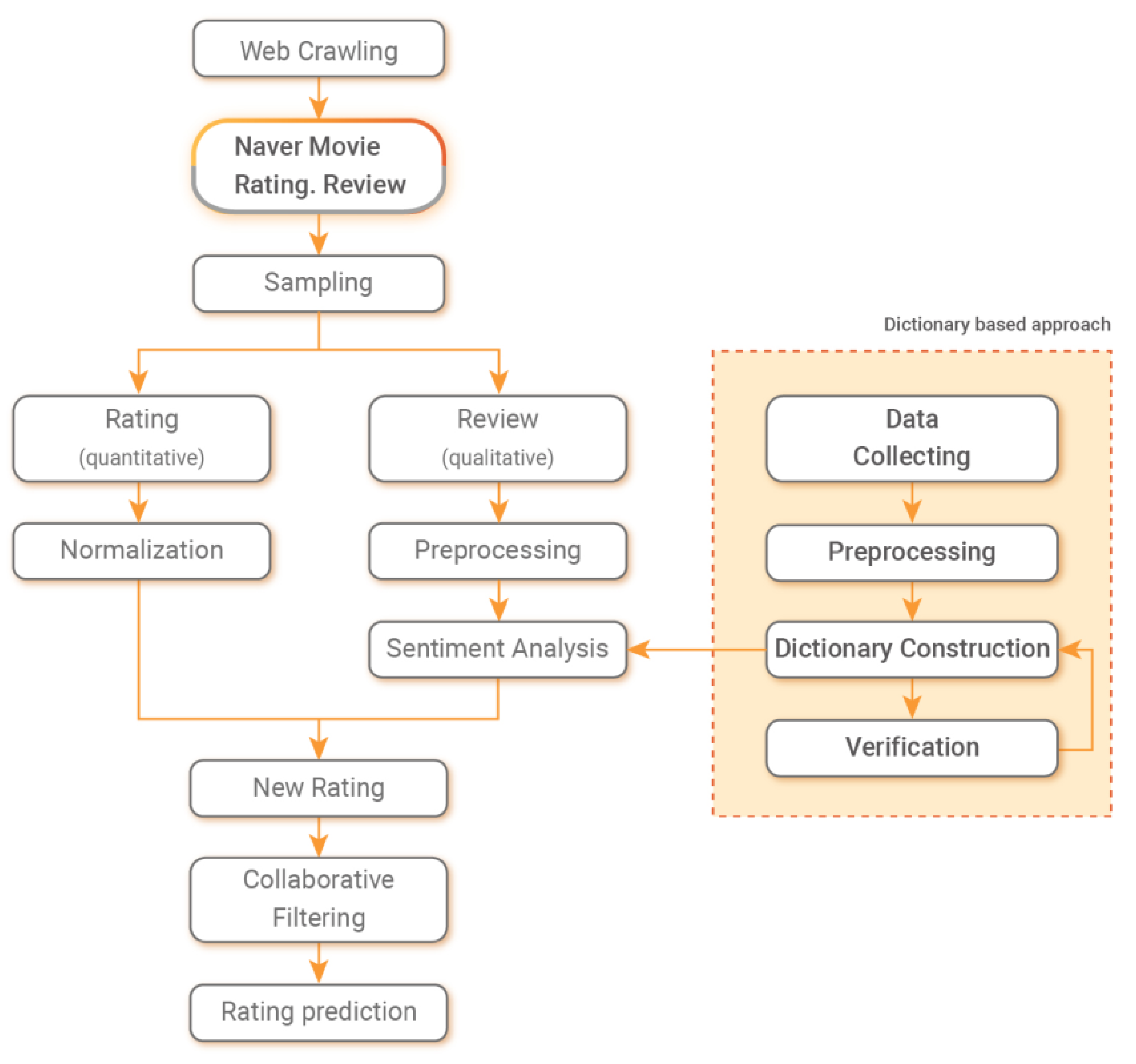
3.5. Step 5, Review-Sentiment Analysis
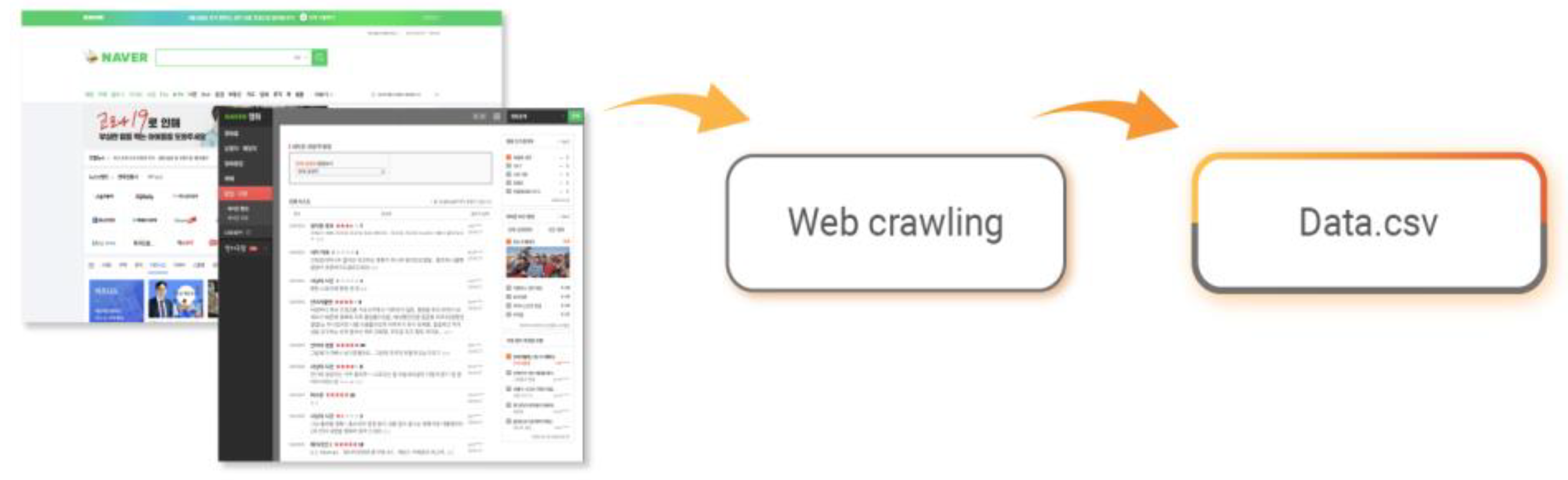
3.5.1. Step 5-1, Review Data Collecting
In constructing the sentiment dictionary, data from NAVER Lab were used as additional data. A total of 200,000 review data were obtained, which had rating integer values between 1 and 10. If the rating score was from 1 to 3, a label of 0 (negative) was assigned to the review, and if the rating score was from 9 to 10, a label of 1 (positive) was assigned. Among the data, 100,000 reviews were extracted with an equal polarity ratio of negative and positive labels. Subsequently, 75,000 movie reviews were used to construct the dictionary and 25,000 movie reviews were used as test data to verify the accuracy of the dictionary.
3.5.2. Step 5-2, Review Data Preprocessing
Morphological analysis was carried out using the same four-step pre-processing procedure. After the morphological analysis, the RHINO library was used to select and extract only the nouns, verbs, and adjectives of the parts of speech from the review data.
To construct a sentiment dictionary, words and phrases were extracted from the training data. In this study, the adjective, noun, and verb parts of speech tags that directly describe and express sentiments, were extracted from the training data to construct word and classification graphs. Among these, the ones that clearly express emotions were defined as sentiment words and sentiment phrases.
Table 2 shows the number of words and phrases extracted to construct the word and phrase graphs, and
Table 3;
Table 4 each display the defined words and phrases.
3.5.3. Step 5-3, Dictionary Construction
The pre-processed review data were transformed into a document-term matrix. During this process, the Term frequency inverse document frequency (TF-IDF) weight method, which indicates the importance and frequency of the word in a document, was used to vectorize the texts.
Figure 5 displays the sentiment dictionary construction flow chart.
The independent variables are the TF-IDF value matrix of review words and the dependent variables are the label values of 0 and 1 of each review. Regression analyses were used to construct the dictionary. After acquiring regression coefficients of each word, the sentiment dictionary was constructed by placing the words into the positive dictionary if the coefficient was greater than 0 and into the negative dictionary if less than 0. However, as the text data lacked structures and had a large number of dimensions, the process of selecting and extracting variables when conducting regression analysis is important to improve the analysis performance. Thus, Ridge, Lasso, and ElasticNet regressions were used among the regression methods [
26].
Ridge regression is a method of shrinking the regression coefficient by penalizing the regression model with a penalty [
27]. Ridge regression is a linear regression that has
- constraints. The ridge estimates are obtained using Equation (4).
From the equation, determines the amount of shrinkage of the regression coefficient. As the value increases, the shrinkage amount also increases, and the regression coefficient value tends to zero.
Lasso regression analysis is a method of shrinking the regression coefficient by penalizing the regression model with a penalty, similar to ridge regression analysis [
28]. This estimation method enables variable selection by making regression coefficient values of insignificant variables, as the lasso estimates are obtained using Equation (5).
As the value of in Equation (2) increases, the value of the regression coefficient tends to zero.
The main difference between the two models of the ridge regression and lasso regression is that the ridge model uses the square of the coefficients; however, the lasso model uses the absolute value. Because the coefficients of each independent variable are close to zero, but not actually zero, the ridge model employs all the independent variables, even if the penalty value is large. However, because some variables become zero if the penalty value is large, the lasso model employs only the selected variables that are not zero.
ElasticNet is an algorithm that combines both ridge and lasso regressions. The ElasticNet estimates are obtained by Equation (6).
The ElasticNet linearly adds penalties of the ridge and lasso methods and adjusts to derive an optimized model. Additionally, it adds an extra parameter of α to differentiate the relationship between the two. In contrast to the ridge and lasso methods, which are adjusted with , parameter α is employed, and the lasso effect increases with an increase in the value of α, whereas the ridge effect increases with the decrease in the value of α.
When using the ridge, lasso, and ElasticNet regression methods, a cross-validation method was used to estimate the shrinkage parameter . After obtaining the optimal value that returns the smallest error through fivefold cross validation, the word that has a regression coefficient value greater than 0 for the given value was classified into the positive dictionary, and the word with a value less than 0 was classified into the negative dictionary, thereby constructing a positive and a negative dictionary.
The words of each constructed dictionary were manually checked and any unnecessary words were removed. For example, if the dictionary contained nouns that were not related to sentiments, such as actor’s names, location names, etc., the corresponding words were removed.
3.5.4. Step 5-4, Dictionary Accuracy Verification
In verifying the accuracy of the dictionary, a test dataset of 25,000 review data was used. Based on the dictionary, sentiment scores of reviews were calculated and classified as positive if the sentiment score was greater than 0, and as negative if less than 0. The sentiment scores are obtained through Equation (7).
To examine the accuracy of the sentiment dictionary, sentiment scores are calculated based on the frequency of the positive and negative words. The sentiment score can range from negative 1.0 to positive 1.0. The words that fall in the score range of +0.1 to +1.0 are identified as positive words, while the words that fall in the range of -1.0 to -0.1 are identified as negative words. Subsequently, the sentiment scores obtained through sentiment analysis are applied to the rating data and new ratings are generated.
As a measure to evaluate the positive and negative prediction results, misclassification ratio was used, and by measuring the accuracy of the confusion matrix of
Table 5, dictionaries with high performance were selected for the analysis [
29].
In this matrix, the values of TP(True Positive), FP(False Positive), TN(True Negative), and FN(False Negative) represent the result values.
TP indicates that the classifier accurately predicted by classifying the positive case as a positive. Conversely, FP indicates that the classifier incorrectly classified the negative case as positive. Similarly, TN denotes that the classifier accurately predicted by classifying the negative case as a negative, while FN denotes that the classifier incorrectly classified the positive case as a negative. Based on the results derived from the confusion matrix, accuracy, precision, and recall can be derived. Equations (8)–(11) respectively express the equations for calculating the accuracy, recall, precision, and F-measures.
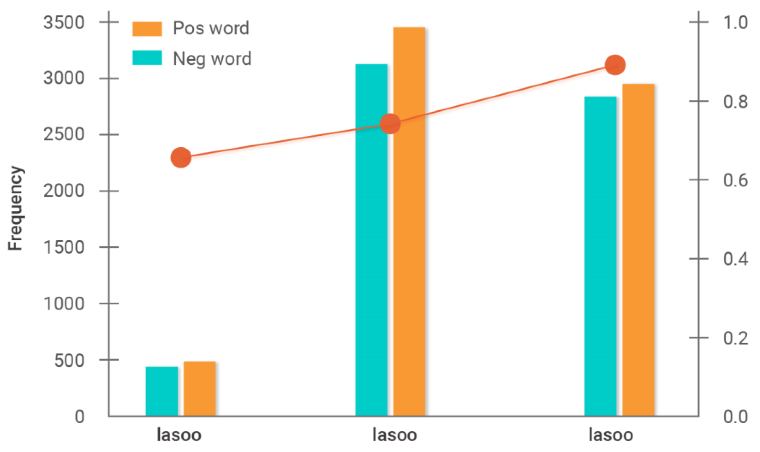
Figure 6 displays the results of calculating the accuracy based on the positive and negative vocabulary frequency of each dictionary and on Equations (7) and (8). Based on the results of the number of words used in the dictionary, the words were more diverse in the way of expressing negative vocabulary than expressing positive vocabulary.
The lasso-based dictionary featured 398 positive sentiment vocabulary and 421 negative sentiment vocabulary, with 70% accuracy. The ridge-based dictionary featured 3164 positive sentiment vocabulary and 3425 negative sentiment vocabulary, with 79% accuracy. When constructing the ElasticNet-based dictionary, α of 0.3 was chosen as it returned the highest accuracy. A total of 2875 positive and 2954 negative vocabulary was extracted with 83% accuracy. As a result, this study used an ElasticNet-based positive and negative dictionary, which had the highest accuracy, for calculating the sentiment scores of user reviews.
Furthermore, this study used the SVM (support vector machine), RF (random forest), and NNet (neural network) algorithms, which are popular methods for recognizing and classifying sentiments. The training and test data were labeled according to the collected sentiment words in the sentiment dictionary. Furthermore, the classifier models were trained using the training data and the trained models were used to classify the sentiments of the test data. The SVM model used a traditional kernel function RBF (radial basis function); the RF model used a total of 500 trees with 10 variables; the NNet used a total of 10 hidden layers. Then, similarly to the earlier regression analysis method of this paper, the 5-fold cross-validation method was used for the classification performance test. For performance measurement, recall, precision, and F-measures were selected to test the accuracy of the model
Table 6 displays the classification performance of each classifier on the sentiment dictionary.
The results of using the general sentiment dictionary and the domain-specific dictionary constructed for analysis identified the following distinctions. Except for the analysis results of the NNet model, the recall values were generally higher than the precision values when using the general dictionary, while the precision values were higher than the recall values when using the sentiment dictionary. Additionally, the dictionary returned a higher F-measure due to the smaller difference between the recall and precision than did the general sentiment dictionary. These results suggest that the constructed dictionary yielded a more stable and accurate sentiment analysis result.
3.7. Step 7, Rating Prediction
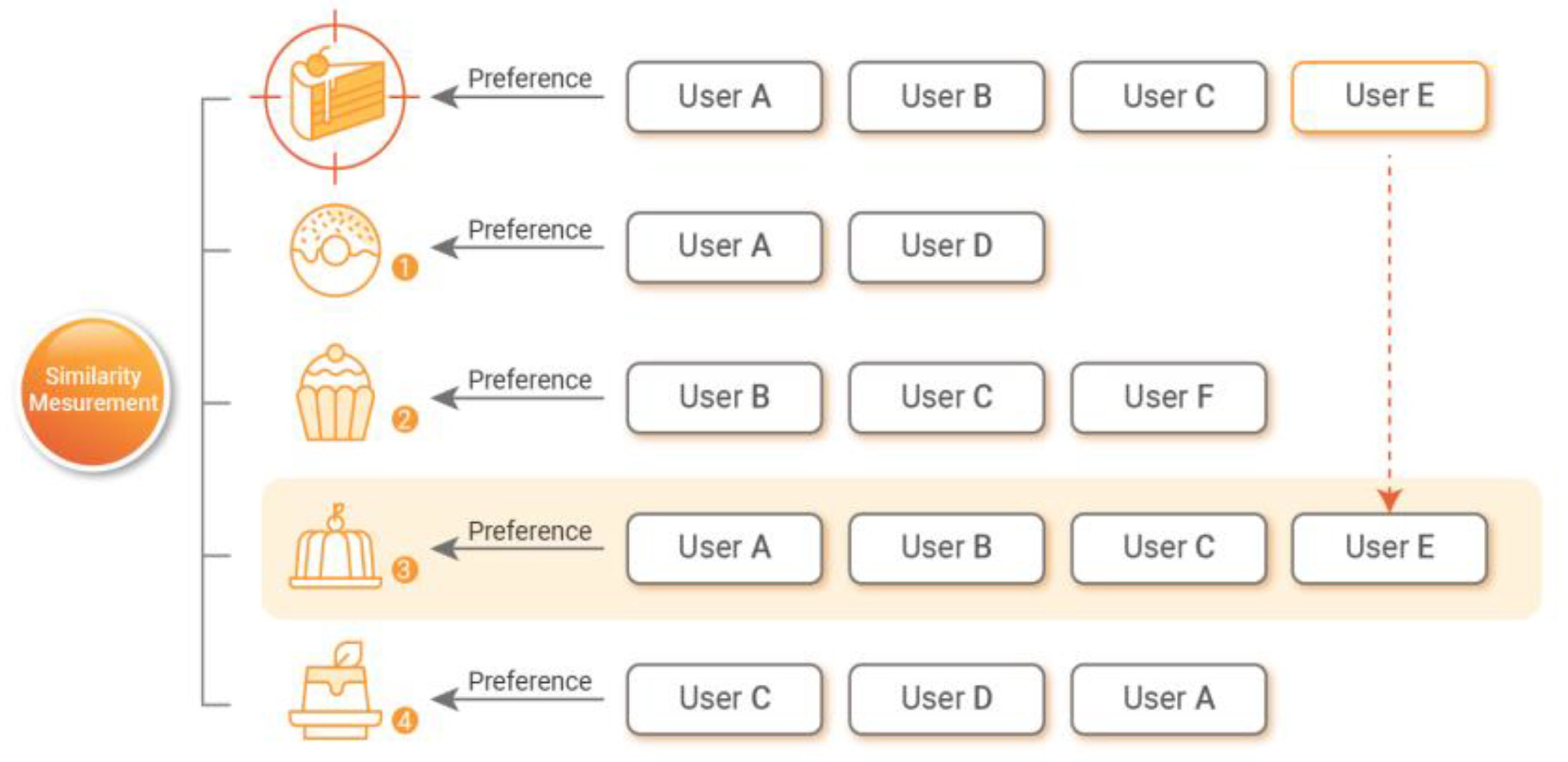
In predicting user ratings, user-based and item-based filtering of model-based collaborative filtering and SVD and SVD++ algorithms, which are popular algorithms of model-based matrix factorization, were used.
After selecting neighboring users who have similar preferences as the target user, based on the rating information entered by the user, user-based collaborative filtering is a method of providing recommendations to a user with items that are commonly preferred by neighboring users. The most important step in predicting ratings through user-based collaborative filtering is calculating the user similarities. The similarity between the two users
a and
b,
, is obtained by Equation (12).
Here, I denotes the entire set of items, denotes the rating score given by user a on item , and indicates the average rating score of all items that user a has rated. Once the users with similar preferences are selected through the similarity measure, the user rating is predicted based on their purchase history, using the weighted sum method.
The predicted rating that user
would provide on the item
i is obtained through Equation (13).
Further, indicates the average score of all items given by the recommendation target user, denotes the average score of all items given by the other user, and represents the weight of the similarity between the user u and recommendation target user a, where a higher similarity returns a larger weight.
In the item-based collaborative filtering, a specific item is selected as a standard, and then a neighboring item with similar user rating scores is selected. Consequently, based on the neighboring item rating score, a rating that the target user might have for the specific item is predicted. The similarity between the two items
and
,
is obtained by Equation (14).
Here, U indicates the set of all users who rated both items and , represents the score on item given by user u, and represents the average score on item given by all users.
The item-based collaborative filtering predicts rating scores through a simple weighted average method, as shown by Equation (15).
Here, and denote the average score of all items given by the recommendation target user and the other user, respectively. Further, uses the weighted similarity between the item to be predicted and the other item to calculate the prediction value by reflecting the rating of the similar item to the item to be predicted.
Among the model-based matrix factorization methods, SVD and SVD++ are the most widely used methods in collaborative filtering. SVD is a method of decomposing a matrix into a product of any matrices. A singular value decomposition on matrix M,
, of all users and items can be expressed as the product of three matrices, as shown by Equation (16).
In the equation, denotes a user matrix, denotes the diagonal matrix entries with singular values in diagonal terms, and represents a movie matrix.
However, as the matrix M is a sparse matrix, there is a probability that SVD may not be defined, owing to many empty values (missing values) that are not provided by the user. To address this problem, a normalized model, Equation (11), is used to predict the rating by deriving a factor vector that minimizes the error function, based on the ratings given by the user.
For the method of minimization, SGD is used to calculate the prediction error, and by adjusting the parameters,
can be predicted through Equations (18) and (19).
In contrast to SVD, which considers explicit feedback information only, the SVD++ method considers both implicit and explicit feedback information.
Based on the SVD method, the characteristics of all the items are reflected in SVD++, regardless of having user rating scores or not. The rating prediction using the SVD++ method is obtained using Equation (20).
The rating prediction value can be derived by the sum of and , , which is the average rating of all data and individual bias values on users and items, respectively. To include the additional association between the user and the item, the explicit rating data matrix and the implicit rating data matrix were decomposed based on SVD. Subsequently, by searching for a low-dimensional hidden space that collectively expresses both the user and item, d-dimensional latent vectors for the item and for the user, were obtained. is characterized by the user, with preference on the item, as a vector. is an attribute that describes the user u.


