Article

Empirical Research on the Fama-French Three-Factor Model and a Sentiment-Related Four-Factor Model in the Chinese Blockchain Industry

1
International Business School Suzhou, Xi’an Jiaotong-Liverpool University, Suzhou 215123, China
2
School of Computing, Engineering and Digital Technologies, Teesside University, Middlesbrough TS1 3BX, UK
3
Department of Computer Science and Information Engineering, Asia University, Taichung 400-439, Taiwan
4
Department of Medical Research, China Medical University, Taichung 400-439, Taiwan
5
School of Mathematics and Big Data, Foshan University, Foshana 528000, China
6
John Molson School of Business, Concordia University, Montreal, QC G1X 3X4, Canada
*
Author to whom correspondence should be addressed.
Sustainability 2020, 12(12), 5170; https://doi.org/10.3390/su12125170
Submission received: 2 April 2020 / Revised: 9 June 2020 / Accepted: 11 June 2020 / Published: 24 June 2020

Abstract

:
As one of the most significant components of financial technology (FinTech), blockchain technology arouses the interests of numerous investors in China, and the number of companies engaged in this field rises rapidly. The emotion of investors has an effect on stock returns, which is a hot topic in behavioral finance. Blockchain is an essential part of FinTech, and with the fast development of this technology, investors’ sentiment varies as well. The online information that directly reflects investors’ mood could be utilized for mining and quantifying to construct a sentiment index. For a better understanding of how well some factors adequately explain the return of stocks related to blockchain companies in the Chinese stock market, the Fama-French three-factor model (FFTFM) will be introduced in this paper. Furthermore, sentiment could be a new independent variable to enhance the explanatory power of the FFTFM. A comparison between those two models reveals that the sentiment factor could raise the explanatory power. The results also indicate that the Chinses blockchain industry does not own the size effect and book-to-market effect.

1. Introduction

Financial technology (FinTech) consists of several technologies, such as blockchain, cloud computing, big data, and machine learning. Blockchain is an advanced technology extracted from the bitcoin, which was first promoted by Nakamoto [1]. As one of the most innovative and important components of FinTech, it could now tackle challenges such as digital currency, asset securitization, cross-border payment and settlement, and insurance management. As part of FinTech, blockchain has produced a series of extremely promising applications because of its characteristics, such as decentralization, immutability, and anonymity. Blockchain can not only play a role in FinTech, but can also be applied to diverse industries, such as supply chain, intellectual property, estate, and the Internet of Things (IoT). Blockchain technology is highly valued in China. Even the People’s Bank of China (PBOC) began planning to issue CBDC (Central Bank Digital Currency) based on blockchain technology, and the excellent design has been basically completed [2]. Mu et al. claim that the People’s Bank of China owns the most blockchain patents among central banks in the world [3]. Due to the innovative nature of this technology and the high level of interest, the number of companies in this field is also increasing. It is necessary to detect the value of these firms to understand this industry better.
This paper will try to make use of the FFTFM (Fama-French Three-Factor Model) for the analysis of stocks of Chinese blockchain firms and to detect the existence of size effect and book-to-market ratio effect (BM effect) in this field. The capital asset pricing model is a popular topic attracting numerous researchers for a long time. Markowitz first proposed portfolio theory to balance the risk and return [4]. Sharpe, Lintner, and Mossion built the capital asset pricing model in the 1960s, and this model considers the market return as the unique variable to explain the return. Fama and French proposed the FFTFM, that adding size factor and book-to-market ratio factor into the CAPM (Capital Asset Pricing Model) enhances the explanatory power [5]. After the model was released, Chinese researchers began to utilize the FFTFM to analyze Chinese stock market performance and found it gains a better result than CAPM [5,6,7,8]. Some studies pay attention to the stock market, for instance, the stocks belonging to the A-shares’ market and Growth Enterprise Market [9,10]. Some Chinese researchers focus on a particular industry via the FFTFM, such as the real estate industry, the electric power industry, steel industry, and bank industry [11,12,13,14]. It could be noticed that many studies emphasize the traditional industry [12,14], whereas the blockchain industry is an innovation and the research of implementation of FFTFM in this field is lacking.
Blockchain owns its noticeable position, especially when it comes to concepts like FinTech. There is a saying that “one day in the blockchain industry, one year in real life”, which reveals the extremely rapid changes in this field. Blockchain technology was first applied in the financial field. Since it revolutionizes centralization and simplifies a series of the transaction process, it is recognized as a particularly useful tool of FinTech, which arouses a lot of interest. The rapid development also has an impact on investors’ expectations and sentiment to the blockchain companies including but not limited to the firms that take blockchain as FinTech, and the relationship between emotion and stock return is an indispensable topic of behavioral finance.
Behavioral finance researchers study the impact of capital market participants’ psychological and behavioral characteristics on capital markets based on the assumptions of limited arbitrage opportunities and bounded rationality. The “emotion” in psychology is the expression of external attitudes generated by individual cognitive processes. Investor sentiment in behavioral finance is caused by investors’ limited rationality and can be interpreted as investors’ expected bias, subjective preferences, investment beliefs, and speculative needs. When investor sentiment affects enough investment demand, it will cause the stock price to deviate from its value. According to empirical studies, investor sentiment has an essential impact on financial behaviors such as stock price and income fluctuations, stock market anomalies, and corporate investment decisions and earnings management [15,16]. Liu and Zhang summarize that the Chinese stock market is mainly composed of individual investors with relatively weak investment skills, keen subjective awareness, and low-risk perception ability [17]. Investors are more inclined to pursue short-term capital gains and are keen on short-term investment projects to gain speculative profits. This determines that investor sentiment owns a more powerful influence in China than in mature capital markets.
Under this background, this paper tries to investigate the influence of Internet information related to the stock performance by mining and quantifying Internet public opinion information. Then the sentiment factor would be added into the traditional FFTFM for research.
The data are collected from the China Stock Market Accounting Research platform and China Research Data Services platform. Sentiment factor results from the Guba public comments of each stock by online users. Stocks that related to blockchain technology, including but not limited to the listed firms that treat blockchain as FinTech, would be grouped to construct portfolios with different characteristics for the research. While comparing the results of the FFTFM and improved four-factor model, the sentiment factor could present a better explanation of the return of Chinese blockchain stocks. It also notices that size effect and BM effect could not be found in this industry, and the portfolios constructed by big-size companies and low book-to-market ratios companies gain the best return.
Due to the creativity and the bright prospect of blockchain technology, this paper focused on Chinese listed firms related to blockchain technology and demonstrated the valuation via the FFTFM, which is supposed to describe the risk yield characteristics of the blockchain industry in China. Many scholars have studied China‘s asset pricing based on FFTFM. This paper also drew on the FFTFM to empirically research the Chinese A-share market, to try to explain the stock performance of the Chinese A-share blockchain firms and verify whether the industry has scale effects, value premium effects, and profitability effects. We concluded that the BM effect does not exist in the Chinese blockchain industry. We also built a sentiment factor using data mining to improve the traditional FFTFM in order to present a better explanatory power for this industry.

2. Literature Review

2.1. Fama-French Model Research

Fama and French found that the beta value of CAPM could not explain the difference of excess return, so they proposed a three-factor model that divides the main factors into three factors, namely market factor, scale factor, and value factor, for a better explanatory power of excess return [4]. In order to explore whether the model can be applied to the stock markets of other countries, Fama and French studied the stock returns and pricing factors in different countries and claimed that FFTFM is better than CAPM [18].
Carhart believed that the FFTFM could not explain the difference of excess returns well and added a new variable-momentum factor to construct the Fama-French four-factor model [19]. Xu and Xiong used A-share listed companies as samples from 2004 to 2005 and found that the four-factor explanatory ability has been improved but cannot fully explain the stock fluctuations in yield [20]. Xue and Guan conducted empirical research through a four-factor model and found that only a few funds can perform slightly better than the whole market index [21]. This paper aimed to construct a model based on FFTFM with a sentiment factor and to detect a more explanatory power, which has a similar purpose as the Carhart model.
Fama and French analyzed profitability and investment information and added them to the FFTFM to construct a new Fama-French five-factor model (FFFFM) [22]. However, the FFFFM is still an imperfect model. Fama and French found that the FFFFM mainly has two defects: The first is that the model lacks the ability to describe the average return of small stocks, and the second weakness is that the HML (High Minus Low) factor is a redundancy factor. Racicot et al. studied the FFFFM with traditional illiquidity measures and found the weakness of this model, especially for the endogenous illiquidity measures [23]. The robust instrumental variables (RIV) algorithm conducted by GMM (Generalized Method of Moment) was taken into consideration for correction. Racicot et al. transferred FFFFM into the dynamic specification and used Kalman filtering and a recursive robust instrumental variables (IV) algorithm to detect the estimation of alpha and beta [24]. They noticed that illiquidity is a significant factor in the Kalman filter approach and that market risk premium is the only effective factor in a dynamic context based on the GMM approach.
Sembiring applied the Fama-French model in the Indonesian securities market under market overreaction conditions and found that the market, size, and value factor are accurate to explain portfolios’ returns [25]. Cox and Britten utilized the FFFFM in the Johannesburg securities market and concluded that size and value factors are significant, but the market factor presents a negative relationship [26]. Bangash, Khan, and Jabeen disagreed that size pattern performs well by empirical research on the Pakistan equity market [27]. In China, scholars not only use the FFTFM to investigate the Chinese stock market but also on the replacement of indicators based on the combination of the Chinese stock market’s actual situation. Tian, Wang, and Zhang compared the FFTFM between the securities market of China and the United States [28]. They concluded that the FFTFM could explain the excess returns of the two countries’ investment portfolios, whereas their applicability in the Chinese and American stock markets is different. The Chinese market risks are more significant than other factors, and SMB (Small minus Big) has explanatory power for small-cap stocks. Yang and Fan indicated that the FFTFM is interpretable to the stock markets of developed and developing countries [29]. Several researchers use the FFTFM application in the Chinese securities market to test the effectiveness of the whole market [9,30,31]. Liu, Zhu, and Li argued that the FFTFM is suitable for China’s Growth Enterprise Market [10]. Yin added the sentiment factor into the Fama-French model and found that prices of small-cap stocks, high P/E (Price/Earnings) ratios, and high-priced stocks are more sensitive to investor sentiment [32]. Hu, Tu, and Zhu believe that the five-factor model of Fama-French stock pricing is suitable for use in China’s stock market [33]. Yuan and Cong found that the FFTFM is suitable for the listed companies in the Chinese HA-DA-QI (Harbin-Daqing-Qiqihar) region [34]. For the stock returns in Chinese, a particular industry, some researchers take the FFTFM to explain the returns. You found the market factor effect and BM effect in the estate industry and Cheng and Fang conducted an empirical research of stock returns in the auto industry [11,35]. For energy listed companies, Li and Zhao pointed out that the FFTFM model applies to the prediction of market returns of China’s listed power companies and that FFTFM could also be used in Chinese iron industry [12,13]. Gou, Wang, and Zhu drew the same conclusion that small-cap stocks own scale effects, and stocks with high book-to-market value ratios have BM effect [14,36].

2.2. Conventional Investor Sentiment Research

Behavioral finance arouses numerous academics’ interest and they hope to find a principle for better decision making by using investor sentiment. Baur, Quintero, and Stevens used stock market data from 1986 to 1988 to explore the relationship between investor sentiment and linkage with the 1987 securities’ market crash [37]. Mehra and Sah summarized the three conditions in which the investor sentiment affects the stock price in the arbitrage market: Firstly, there is a systematic fluctuation of investor sentiment; secondly, investors make decisions based on emotions; thirdly, investor ignores the subjective influence brought by emotions [38]. Brown and Cliff collected data and compiled investor sentiment index [39]. The study found that the lag effect of market yield has a more significant impact on investor sentiment, but, in turn, investor sentiment is not efficient in predicting market returns. Cheng and Liu used a blue-chip index to reflect the bullish situation and found that the stock market’s mid-term sentiment was more affected than the short-term sentiment [40]. Wang, Zhao, and Fang claimed that investor sentiment leads to share prices in the early stage of IPOs (Initial Public Offering), which will cause listed companies to use investor sentiment to maximize profitability [41]. Wen et al. used the Shanghai Securities’ Market data to construct an investor sentiment index to study the characteristics of investor behavior under different emotions [42].

2.3. Investor Sentiment Research Based on Internet Information

Currently, how to use social network information to predict economic behavior has gradually become one of the research hotspots in various fields. Tetlock uses the one column of the Wall Street Journal as the investment sentiment analysis basis, and analyzes the relationship between investor sentiment and stock market returns [43]. He believes that the large fluctuations in investor sentiment will cause an increase in volume, and pessimistic forecasts will lead to a fall in stock prices. Chen et al. indicated that online information helps investors make better financial decisions [44]. Meng, Meng, and Hu constructed the investor sentiment index using factor analysis, based on the data of CSSCI (Chinese Social Sciences Citation Index), Sina Weibo text, and Baidu’s keyword recommendation system [45]. Luo, Wang, and Fang considered investor sentiment index when establishing the CAPM, and the investor sentiment index was constructed on the sentiment analysis of the stock forum posting [46]. Investor sentiment against the stock index based on the ordinary linear regression model was found. Xu uses text analysis and machine learning to construct a new investor sentiment indicator system based on Sina stock evaluation information and a long-term survey [47].

3. Data

3.1. Stock and Financial Data

This paper selected listed blockchain companies in Shanghai and Shenzhen stock markets. The Special Treatment (st) company cannot be considered as a regular listed company because of its business difficulties, so the data only included non-st companies’ data. Because the data of listed blockchain companies included in the Wind blockchain index were complete since 2016, and to test the authenticity and comprehensiveness of the samples, monthly stocks’ data during June 2016 to June 2019 were collected from China stock market and accounting research database and Chinese research data services platform (CNRDS). After screening, there were 50 sample companies. A large sample time interval, with sufficient and new sample data, could provide a practical and meaningful result.
This paper selected the monthly information of stocks related to the Chinese blockchain industry from June 2016 to June 2019, which was collected from the Chinese stock market and CNRDS. These stocks included, but were not limited to, some listed companies that use blockchain as a FinTech.
The way to determine whether a company is involved in the blockchain industry is based on the components of Wind’s blockchain industry index. If a firm was collected as a component of the index, this firm was considered for the research. There was an overlap between the stocks belonging to the blockchain industry index and the stocks belonging to the FinTech index.
The traditional Fama-French model will reclassify the portfolios at the end of June each year, but to better reflect the performance, this paper regrouped the portfolios monthly. The reason is that the blockchain industry in China is an emerging industry, and several companies are embracing this innovative technology, including, but not limited to, FinTech firms. Other companies involved in FinTech also show the same trend. In 2016, there were merely eight listed firms related to blockchain technology according to Wind database, whereas there were more than 150 firms in 2019 [48]. More data details will be shown in Section 3.1.1, Section 3.1.2 and Section 3.1.4.

3.1.1. Stock Returns

The stock returns were selected by the monthly return that after cash dividend reinvestment. Transaction costs was not considered. Stock returns are the basic element for constructing SMB and HML factors [49].

3.1.2. Market Returns

Monthly market returns would be seen as a market index, which is comprehensively calculated based on the returns of China A-shares market, B-shares market, and China’s growth enterprise market. This is due to the complexity of the blockchain industry in China. These listed companies have different characteristics and are distributed in different stock markets. Some of them are FinTech firms. Therefore, this comprehensive index can more comprehensively and objectively reflect the overall price change trend of the market and provide investors with more valuable indicators. This element could reflect the situation of the whole market, which is also an essential data for calculating beta [49].

3.1.3. Risk-Free Rate

In practice, there is no absolute risk-free interest rate. Researchers choose those financial products with better liquidity and less default risk to represent the risk-free interest rates, such as the national debt rate and bank savings deposit rate. The Chinese banking system is dominated by state-owned banks with little default risk, no market segmentation issues, or any individual or corporate institution that can deposit in the bank [50]. This paper intended to select the one-year-term savings deposit interest rate and convert it into a monthly return rate by using the continuous compounding method.

3.1.4. Size

The size of a listed company is determined by its market capitalization, obtained by multiplying the stock price by the number of shares outstanding. According to China’s unique conditions, stocks are divided into tradable shares and nontradable shares. Due to the special historical background of the restructuring of state-owned enterprises, the existence of nontradable shares is a major feature of China’s securities market and nontradable shares cannot be circulated on the secondary market [51]. So only tradable shares will be used and market capitalization calculated by the tradable shares as well.

3.1.5. Value

The measurement of the value of the company is the number of book equity to the market value of equity. The financial statement of the listed company does not directly present this number, but it could be gained from price-to-book value. This paper took the reciprocal of the PB (Price-to-Book) value on the last trading day of each month.

3.1.6. Sentiment Data

There are various resources to construct investor sentiment factors. Zhang and Liu summarized that the simple sentiment index mainly adopts a direct survey method or data mining method, and compound indicators are constructed by selecting multiple single objective indicators, or a combination of single objective indicators and subjective indicators to construct investor sentiment [52]. This paper used the data mining method, and Guba comments were used to present investors’ sentiment. Unlike news reports from newspapers or traditional news websites, Guba is a free medium, and the content of their posts is mainly the expression of investors’ subjective wishes, which are relatively random and irregular. For example, Guba comments may contain a few simple words, or some irrelevant expressions and meaningless text expressions. These noises will affect the accuracy of our sentiment judgment on posts. Comments on blockchain companies, including the firms, treat this technology as FinTech and would be collected for further analysis.
There are several platforms for analyzing the text and extracting the emotional tendencies from the content, for example, cloud natural language from Google, Baidu AI (Artificial Intelligence) platform, and Yuyi data platform. In order to keep data consistent, the Guba media data analysis database from the Chinese research data services platform was used in this paper. According to the Guba database description, the platform uses a supervised learning model to judge the post’s sentiment. The application of supervised learning in the post classification of the database includes the following steps: ① Define the categories (including positive, negative, and neutral) in advance, manually label the content of the posts, and obtain positive, negative tendency. Score 1 is positive, −1 is negative, and 0 is neutral. ② Automatically obtain data from a dataset with category information. This part of the data is called “training data”. ③ Supervised learning algorithm support vector machine is introduced to learn the classification model on the training dataset. Use classification models to predict the categories of a test dataset automatically. It is noticeable that the Guba comments data from the Chinese research data services platform were merely from 2008 to 2018, so the 2019 comments data were collected from the China stock market and accounting research database.

4. Methodology

4.1. Build Portfolios According to Size and Value

The stocks will be grouped monthly from two dimensions, size and value.

4.1.1. Size

There are many ways to determine in which group the company should be involved, and there are various ways to deal with it. Fama and French divided the stocks from three American stock exchanges into a small or big group based on the median of the size factor [5]. This paper used the FFTFM division method. After sorting the circulating market capitalization in ascending order, the stocks were evenly divided into two groups: Small (S) and big (B).

4.1.2. Value

Fama and French sorted the book-to-market ratio in ascending order and divided the sample data into low (L) group, medium (M) group, and high (H) group, according to the proportions of 30%, 40%, and 30%, which are called growth group, medium group, and value group [5]. Since the number of blockchain companies change rapidly, including but not limited to the firms that take blockchain as FinTech, so, based on the traditional Fama-French division method, the number of shares in a certain group might be zero. In order to deal with this issue, the stocks were evenly classified into two groups, high group (H) and low group (L). In the future, there will be more companies using blockchain technology and more companies embracing FinTech. By then, this weak point can be compensated.

4.1.3. Portfolios

After the above two classifications, each stock had two indicators: Size and value. Those stocks will be cross-combined to build four portfolios based on those two dimensions. They are S/L, S/H, B/L, and B/H. The research on the Fama-French pricing model was based on the data of these four portfolios.
The details of these four portfolios are:
  • Portfolio S/L: Refers to those stocks which both belong to the small-size group and low book-to-market ratio group at the same time.
  • Portfolio S/H: Refers to those stocks which both belong to the small-size group and high book-to-market ratio group at the same time.
  • Portfolio B/L: Refers to those stocks which both belong to the big-size group and low book-to-market ratio group at the same time.
  • Portfolio B/H: Refers to those stocks which both belong to the big-size group and high book-to-market ratio group at the same time.

4.1.4. Construction of Independent Variables

Ri

Ri is the return of the portfolio that is calculated according to the ratio of the circulation market value of each stock to the sum of the circulation market value of the combination.

Market Risk Premium Factor (Rm-Rf)

The market risk premium is obtained by subtracting the risk-free interest rate from the market rate of return. As mentioned above, the market return (Rm) is a monthly return of A-shares, B-shares, and China growth enterprise market. It is a comprehensive monthly return that is considered after cash dividend reinvestment and obtained by using a weighted average market capitalization method. The risk-free rate is the coupon rate of the one-year bank saving deposits and then turns an annual risk-free interest rate into a monthly one.

SMB

SMB factor is obtained by comparing the average portfolio return of a small-sized company and the average portfolio return of a big-sized company. This factor measures the difference in returns due to the size of the listed companies. The construction method is to sort all companies according to market capitalization from low to high, select the first 50% of the stocks to form a small market value group, select the last 50% of the stocks to form a large market value group, and calculate the return of small market value group and the return of large market value group, respectively. Then calculate the difference between those two return rates. Repeat the above process every month to get the SMB factor sequence.
The specific calculation formula is as follows:
S M B t = ( S / L ) + ( S / H ) 2 ( B / L ) + ( B / H ) 2

HML

HML factor is obtained by comparing the monthly return rate of the high book-to-market ratio portfolio and the monthly return rate of the low book-to-market ratio portfolio. This factor measures the difference in returns due to different book-to-market ratios of listed companies. The construction method sorts all companies according to the book-to-market ratio from high to low, selects the top 50% of the stocks to form a group with a high book-to-market value ratio, and selects the bottom 50% of the stocks to form a group with a low book-to-market value ratio. Then calculate the market-weighted return of the two groups, respectively. Repeat the above process every month to get the HML factor sequence.
The specific calculation formula is as follows:
H M L t = ( H / S ) + ( H / B ) 2 ( L / S ) + ( L / B ) 2

Sentiment Factor

Antweiler and Frank introduced a method to measure the effect of investors’ sentiment [53]. Bu et al. proposed a measure of investor sentiment that integrates bullish and bearish expectations of investors based on the Guba comments and naive Bayesian method [54]. This paper referred to this method to construct the model for analyzing the negative or positive sentiment based on the Guba comment website. The formulation is:
S e n t t = M t p o s M t n e g M t p o s + M t n e g
The M t c = i D ( t ) w i x i c means the sum of one emotion during the period D(t). The “c” belongs to positive, negative, or neutral. The x i c means if a comment “i” is one of “c”, then x i c equals 1. If a comment “i” is not one of “c”, then x i c equals 0. The “pos” represents positive emotions, “neg” represents negative emotions, and “neu” represents neutral emotions. The sentiment index “ S e n t t ” is between −1 to 1, which indicates investor expectations. Every stock has a “Sent” value every month. According to which portfolios they belong (S/L, S/H, B/L, B/H), the “sent” value of each portfolio will be obtained.

Fama-French Model

After collecting and processing the data above, the traditional Fama-French model could be presented:
E ( R i ) R f = b i [ E ( R m ) R f ] + s i E ( SMB ) + h i E ( HML )
The regression equation of the model is expressed as follows:
R i R ft = α i + β i ( R mt R ft ) + s i SMB t + h i HML t + ε it
According to the idea of the FFTFM, based on the model, the sentiment index reflecting investor sentiment was constructed according to the above sentiment analysis method. Then, add the sentiment factor to the model, and finally get a four-factors model:
R i R ft = α i + β i ( R mt R ft ) + s i SM B t + h i H M L t + s e n t i S e n t i m e n t i t + ε i t
R i R ft is the excess return on portfolio “i”. It is the difference between the weighted return of portfolio “I” and the risk-free rate during the same period ‘t’.
R mt R ft is the difference between the market return and risk-free rate during the same period “t”.
SM B t is the difference between the portfolio returns of the small companies and the portfolio returns the big companies constructed during the period “t”.
H M L t is the difference between the return of portfolios with high book-to-market ratio companies and the return of portfolios with low book-to-market ratio companies during the period “t”.
S e n t i m e n t i t is the sentiment score of the portfolio “i” during the period “t”.

5. Analysis of the Model

5.1. Descriptive Analysis

Based on the collected data and indicators constructed before, we could perform descriptive statistical analysis. Related data processing was conducted in Python.
Table 1 shows the basic monthly returns of four different portfolios from 2016 to 2019, and it could be noticed that portfolios with low book-to-market ratios had a positive average return. Additionally, the investment portfolio with the lowest average rate of return was B/H, which was −0.01115. Portfolio B/L owned the highest average rate of return, which was 0.01505. This portfolio had the lowest standard deviation, indicating the smallest fluctuation of the performance. S/L portfolio owned the highest standard deviation, which meant that the small-size company with low book-to-market ratios carried the most top variations. Table 2 shows the correlation between parameters and portfolios’ returns. The correlation coefficient between SMB and market premium was 0.19, indicating that the two were positively correlated, where that between HML and market premium was −0.1, showing the negatively correlated.

5.2. Market Risk Factor

Generally, the trend of market risk factors is the same as the trend of the average return of the four portfolios. Among them, the market risk factor better reflects the changing direction of the S/H, B/H portfolio. Changes in other combinations can also be presented, but there will be some discrepancies in specific periods. The portfolio S/L and B/L excess market factored a lot during the period from February 2018 to April 2018. This showed that the market risk factor was one of the essential variables to explain the difference in stock returns, but it was not enough to rely on the market risk factor alone to explain the changes. This also reflected the defects of the CAPM model from the side, as shown in Figure 1.

5.3. Size Factor

Figure 2 and Figure 3 show the comparison of portfolios with different companies’ size, given the same book-to-market ratio. The orange line presents the portfolios constructed by the big companies, while the blue line displays the one built by the small companies. From June 2016 to February 2019, the trend of the monthly average return of a portfolio with large-size listed companies was consistent with the direction of the one constructed by small-size firms. After February 2019, the average monthly yield on stocks of small-size listed companies was higher than the portfolios of large-scale listed companies. This may be because there were fewer companies engaged in the blockchain industry before 2019, and the size of the company cannot be an essential factor affecting the portfolio yield. After 2019, there were more than 50 companies engaged in the blockchain industry, which more clearly reflected the difference in yields caused by size. This trend may be because blockchain is still a new technology, and the number of companies, including the firms that treat blockchain as FinTech, was relatively small in the early stage.

5.4. Related Test

ADF (Augmented Dickey–Fuller) Test

Generally, the first step is to perform a stationary test when studying on a time series data. The Fama-French model is based on the return of stocks, which is a kind of time series dataset. In addition to the method of visual inspection, the more commonly used statistical test method is the augmented Dickey–Fuller (ADF) test, and it is an extended form of Dickey–Fuller test. The ADF test is also known as the unit root test. If the significance test statistic obtained is less than three confidence levels at 10%, 5%, or 1%, then there should be 90%, 95%, or 99% certainty to reject the null hypothesis accordingly. Since the difference between the FFTFM and the improved four-factor model is adding a new independent variable “sentiment”, the selected stocks remain, and the classification method does not change as well. Therefore, it merely needs to test the stationary of returns of each portfolio. The ADF test is suggested to be conducted in Python using the “statsmodels” package, and the results are delivered in Table 3. As shown in Table 3, the return of eight portfolios all passed the ADF test. The t-values of them were −5.4165, −5.0223, −4.3714, and −5.2175, respectively, and all p-values were equal to zero. As the null hypothesis was rejected, there was no unit root in any time series data. The stationary data could be taken into further research.

5.5. Autocorrelation

Autocorrelation refers to the correlation between the expected values of random error terms, and it could harm the effectiveness of the multilinear regression model. So, whether using the traditional FFTFM or the four-factor model, including the new sentiment parameter, it is necessary to test if this situation exists. The first detection method was the standard Durbin–Watson (DW) test, and the results of the test are presented in Table 4. The range of DW was from 0 to 4, and the value of DW close to 0 indicated that the error terms were a positive autocorrelation while the value close to 4 indicated the negative autocorrelation. If the DW value ranged from dL (lower critical value of d) to dU (upper critical value of d), it could not judge whether there was autocorrelation. Moreover, if the DW value was between dU and 4-dU, it could bring greater confidence to conclude the non-existence of autocorrelation. It is required to refer to a list of DW values to acquire the upper limit value (dU) and lower limit value (dL) under different situations for checking the autocorrelation accurately. According to Table 4, there was no autocorrelation in most portfolios. Still, the DW values of portfolio S/L and B/H in the traditional FFTFM could not confirm whether they passed the test. The S/L portfolio in the FFTFM was also unable to recognize if there was autocorrelation. Therefore, Breusch–Godfrey LM (Lagrange multiplier) test was suggested to be considered, and the probabilities of chi2 (Chi-square) were 0.0818 and 0.0847, respectively. The null hypothesis of the Breusch–Godfrey LM test was that there was no autocorrelation. The results of the Breusch–Godfrey LM test also emerge in Table 4, and it can be seen that the probability of all portfolios implied that the null hypothesis was acceptable. There was no autocorrelation in any multilinear regression models.

5.6. Multicollinearity

Multicollinearity means that there is a linear correlation among the independent variables. This situation manifests itself as one independent variable that can be a linear combination of one or several other independent variables. It hurts the regression model. Perfect multicollinearity could result in the non-existence of parameter estimation. Near-extreme multicollinearity allows the estimator of the ordinary least square model to cease to be effective. Simultaneously, the parameter estimator and the significance test would not make sense. It could not obtain a reliable prediction under the multicollinearity. The value of variance inflation factor (VIF) could be used for multicollinearity test. A greater VIF value means a higher probability of multicollinearity between independent variables. The results of the multicollinearity test are shown in Table 5. All independent variables in every regression model could pass the test, and there was no multicollinearity

5.7. Heteroscedasticity

All error terms have the same variance, which is an essential hypothesis of ordinary least squares regression that guarantees a reliable result of parameter estimation. If the error terms own a different variance, it could conclude that heteroscedasticity exists in the linear regression model. There are several test methods for heteroscedasticity, such as the White test, Park test, Gleiser test, Goldfel—Quandt test, and a directly subjective judgment is based on the graph. In this paper, the White test was taken into consideration for heteroscedasticity, and the results are presented in Table 6. The null hypothesis of the White test was there is homoscedasticity, and the alternative hypothesis was that there is unrestricted heteroskedasticity. According to Table 6, the probabilities of all portfolios, be they a three- or four-factor model, were higher than 0.05 overall. It implies that the null hypothesis was accepted and there was no heteroscedasticity in any portfolios.
After conducting the above tests, we could conclude that there was no autocorrelation, multicollinearity, and heteroscedasticity. Further regression analysis was allowed to perform.

5.8. Regression Analysis of the FFTFM

5.8.1. Goodness of Fit of the FFTFM

The sample data obtained through actual observation used in empirical research were all authentic reflections of facts. Therefore, after introducing the sample data into the model, it must be able to describe this part of the objective facts well before the model can be considered meaningful. Therefore, the model after data processing should be able to describe the fact better. The degree to which the model approximates the sample is called the “goodness of fit.” In multiple regression analyses, the determination coefficient R2 is usually used to determine the goodness of fit of the equation. The R2 indicates what percent of the independent variable can explain the dependent variable. The value of R^2 is between 0 and 1. The closer R2 is to 1, the better the model fits the sample data. If the R2 is close to 0, the model fits the fact badly. The regression could be conducted in Python and the results of “goodness of fit” are shown below. Durbin–Watson statistics were also included in the table, indicating no autocorrelation.
The FFTFM model performed relatively well in stocks of China’s blockchain industry, which could provide a reference for other FinTech companies. The S/L group performed best in terms of explaining portfolio returns, explaining 77.7% changes in the stock return. Portfolio B/H owned the worst result, only 45.8%. These results illustrate that more factors could explain that the portfolio return needs to be included in the mode, as shown in Table 7.

5.8.2. Significance Test of the Model

The goodness of fit can only reflect the results of the FFTFM based on the selected data, but cannot describe the overall relationship among the factors. Therefore, it was necessary to perform a significance test on the model to test the degree of approximation of the trend in yields. The universal test for testing the significance of the whole model is the F-test, as shown in Table 8.
Test hypothesis:
Hypothesis 1 (H1).
All coefficients of the regression model are zero, which means that it indicates that the linear relationship of the FFTFM is not significant, and the model is meaningless.
Hypothesis 2 (H2).
At least one of the coefficients are not zero. This shows that the FFTFM has a significant linear relationship, and this model has explanatory power to portfolio returns.
According to Table 8, at a given significance level of 1%, the F statistics of the four portfolios were all greater than the critical value ( F 0.05 ( 3 , 33 ) = 2.89 ). Then the null hypothesis H1 was rejected, which illustrates that at least one of the regression coefficients was significantly different from 0. It can be concluded that the linear relationship of the FFTFM was significant. Besides, the probability value corresponding to the F statistic of each portfolio was equal to 0, which also shows that the overall linear relationship of the FFTFM was highly significant. In short, the FFTFM can better reflect the overall characteristics of portfolio returns, which the companies constructed by the companies related to blockchain technology. It may also provide a baseline for other companies that use blockchain as FinTech.

5.8.3. Significance Test of Coefficients

In the previous section, the F-test of the FFTFM was performed in this paper. The results showed that all four portfolios passed the F-test, which indicates that all factors in the FFTFM (Rm-Rf, SMB, and HML) on stock returns were significant. However, this does not mean that each element in the model (Rm-Rf, SMB, or HML) had a considerable effect on the yield alone. Therefore, it was necessary to test the significance of each coefficient in the model. This paper used the t-test to analyze the impact of a single factor on the stock return in the model.
As an explanatory variable shared by the capital asset pricing model and the FFTFM, testing the coefficient b of the excess market rate of return (Rm-Rf) can analyze whether market risk factors have a significant effect on stock returns.
According to Table 9, the coefficients of all portfolios were positive values, which indicates that the market risk factor was positively correlated with the stock return. Besides, the coefficients of the portfolios all passed the t-test with a significance level of 1%, and the t-values exceeded the significance level of the coefficient that represents the scale factor and the coefficient that means book-to-market ratio factor. This shows that market risk factors had a significant impact on stock returns. However, it is different from the study of Fama and French [5]. They concluded that market risk factors have only weak explanatory power.

5.8.4. Book-to-Market Ratio Factor

The coefficient of the book-to-market value ratio factor (HML) was conducted to test whether there was a significant relationship between the HML and portfolio returns. As shown in Table 9, only the S/L and B/L passed the 1% significance test, and portfolios that were constructed by companies with a high market-to-book ratio performed worse and did not pass the t-test. Fama and French concluded that when the stock has a low book-to-market rate, which is called is a growth stock, the HML factor in the model generally has a negative slope or a decreasing positive slope; when the stock has a high book-to-market ratio, which is called value stock, the HML factor in the model generally has an increasing slope [5]. However, the empirical research of the Chinese companies in the blockchain industry, including which companies take blockchain as FinTech, did not follow this rule, and firms with high market-to-book ratio could not pass the t-test of HML.

5.8.5. Size Factor

This part examines the linear relationship between the independent variable SMB and portfolio returns. Analysis of the results in Table 9 showed that the regression coefficients of the company’s size factor SMB on S/L, S/H, B/L, and B/H were 1.0496, 0.3943, −0.6057, and 0.0496, respectively. The p values of the t-test were 4.916, 1.730, −2.657, and 0.232, respectively. According to the above results, the SMB factor of the three portfolios, S/L, S/H, and B/H, had a positive correlation with the excess return of the portfolio, while the explanatory variable SMB factor of the B/L portfolio had a negative relationship with its performance. According to the t-test results of the SMB factor, the p values of the S/L and B/L portfolios were less than 1%, and the p-value of the S/H was less than 5%. Therefore, the correlation coefficient passed the test significantly, indicating that the SMB factor had a substantially higher positive correlation for small-scale blockchain stock portfolios. The t-value of the coefficient of portfolio B/H was less than the critical value, and the confidence level of the p-value was greater than 10%, which means that the correlation between the scale factor and the return of B/H portfolio was not significant. Since the samples were companies using blockchain, which are one of the components of FinTech, it might present a reference for other FinTech firms.

5.8.6. An Improved Four-Factor Model Based on Fama-French Model

After collecting and processing the data about Guba comments on each blockchain company, the score of the investors’ emotions could be obtained. People generally regard blockchain as an innovative technology, especially when it comes to FinTech. The score of sentiment is a daily series, and it should be turned into a monthly sequence. Moreover, the monthly score of the firms that are in the same portfolio will be average weighted to get the grades of the portfolio’s monthly score. Subsequently, the four portfolios, S/L, S/H, B/L, and B/H, own their sentiment index each month, which could be added into the traditional Fama-French model to construct a new four-factor model. The equation is shown below:
R i R ft = α i + β i ( R mt R ft ) + s i SM B t + h i H M L t + s e n t i S e n t i m e n t i t + ε i t

5.8.7. Goodness of Fit and F Test

Table 10 illustrates the results of the F test and goodness of fit of the four-factor Fama-French pricing model.
The F test results for measuring the significance of the regression equation show that the p-value of F test for the S/L, S/H, B/L, and B/H portfolios was equal to 0 when the number of samples was 150, and the number of explanatory variables was 3. All four portfolios passed the F test at a 99% confidence level, indicating that the four sets of regression equations were highly significant. From this, it was concluded that the independent variable market factor (Rm-Rf), the scale factor (SMB), the value factor (HML), and the sentiment factor (Sentiment) all had significant effects on the dependent variable portfolio yield.
R 2 can be used to test how well the regression equation fits the sample observations. The closer R 2 is to 1, the better the regression fit. The results in Table 10 show that the determination coefficient of the S/L was 0.771, the determination coefficient of the S/H combination was 0.529, the B/L combination was 0.689, and the B/H was 0.514. From the above analysis, it was found that the portfolio with the best fit was a small-scale and low book-to-market value one, and the worst fit was the portfolio constructed by the big-scale and high book-to-market value companies. The fit of the four groups was not very good, so there should be other factors in the market that had higher explanatory power besides three factors.

5.8.8. Parameters’ Analysis

The first is the regression coefficient, and the significance analysis of market returns to the returns of each portfolio. S market portfolio returns are proxy variables for systemic risk; the beta reflects the sensitivity of a single asset or portfolio to market changes. Table 11 shows that the market risk premium coefficient β values of the four portfolios were 1.2245, 1.3174, 1.289, and 1.1852, respectively. The β coefficients were all greater than 0, indicating that the return on portfolios kept the same moving direction as the return of the whole market. The p-values of the t-test of the four stock portfolios were all less than 1%, and the null hypothesis could be rejected at a 99% confidence level. Therefore, it is believed that the linear relationship between the market factor (Rm-Rf) and the portfolio return was significant.
Secondly, the linear relationship between independent variable SMB and portfolio return rate was tested. The results in Table 11 reveal that the regression coefficients of the company size factor (SMB) on S/L, S/H, B/L, and B/H were 1.06, 0.4275, −0.4984, and 0.1167, respectively. The t-values were 4.878, 1.871, −2.203, and 0.56, and the p-values for the t-test were 0, 0.070, 0.035, and 0.579. It illustrates that the SMB factors of portfolio S/L, S/H, and B/H had a positive correlation with the excess return, and the explanatory variable SMB factor of the B/L had a negative correlation with its return. According to the t-test result of the SMB factor, the p-value of the S/L portfolio was less than 1%, and the p-value of the S/H was less than 10%. Therefore, the correlation coefficient passed the test significantly, indicating that the scale factor (SMB) affected small-scale blockchain stocks. The portfolios had a significantly higher positive correlation.
The SMB factor in the B/L portfolio also passed the t-test at the 1% confidence level. Still, the t value of the B/H was less than the critical value, indicating that the correlation between the scale factor of the B/H portfolio and the portfolio’s return was not significant.
Thirdly, the correlation coefficients that showed the BM effect in the four portfolios were −1.1042, −0.0487, −0.8535, and −0.155, in turn. The t values were −5.793, −0.249, −3.922, and −0.872, respectively, with the corresponding p values 0, 0.805, 0, and 0.39. The regression results showed that HML factors of all portfolios had a negative correlation with their return, which is different from the study of Fama and French [5]. According to the t-test results, the t-values of value factor (HML) in S/L and B/L portfolio were greater than the critical value, and these HML factors in the two portfolios passed the t-test at the 1% confidence level. The t-value of HML in portfolio S/H and B/H showed that the HML factors were not allowed to pass the test, which means that the HML factor in portfolios composed of listed firms with high market-to-book ratio owned the very weak relationship with the return of the portfolios.
Finally, the fourth-factor, “sentiment”, was suggested to test. The results in Table 11 reflect that the coefficients “Sentiment” in four portfolios were 0.0351, 0.1054, 0.2469, and 0.1493, in respect, which implied that the sentiment factors in all portfolios had a positive relationship with the return. In brief, the more exciting the investors, the higher the returns of stocks. However, when checking the results from a more detailed perspective, it was not difficult to conclude that merely sentiment factors in portfolios comprised of big-sized firms could pass the t-test at a 10% confidence level. The t-values of sentiment factor of S/L and B/L portfolios were 0.0351 and −0.0487, respectively. So it was no significant relationship between investors’ sentiment and the return of portfolios that were constructed by small-size firms.

6. Conclusions

This paper is relevant to the topic of regression for FinTech, to demonstrate the effective valuation theory conducted in companies embracing FinTech. It focused on the blockchain companies in China, including those which treat blockchain as FinTech, and used the FFTFM to find these firms. It also contained a new sentiment factor collecting from public comments for better explanatory power. After the above descriptive analysis and regression analysis, it could lead to some conclusions.

6.1. Feasibility of FFTFM and an Improved Four-Factor Model

The FFTFM and the improved Fama-French model that added a new sentiment factor both passed the F test. The market factor, size factor, and book-to-market ratio factor in FFTFM owned the explanatory power to describe and review portfolios’ returns. In the improved model, the sentiment factor could also explain the return of portfolios effectively.
It was noticeable that the explanatory power of four portfolios in FFTFM increased when adding sentiment factor, rising from 0.77, 0.509, 0.653, and 0.458 to 0.771, 0.529, 0.689, 0.514, respectively. It revealed that the sentiment factor had a positive effect on the model. All coefficients of sentiment factors in different portfolios were positive, indicating more optimism brings a higher return.
However, there are still some minor flaws that caused the eight portfolios’ R-square to be not as good as the expectation: The best goodness-of-fit value was 77.1%, and there could be more explanatory variables to review the return of portfolios.
Additionally, to guarantee the reliability of the regression results, it was indispensable to test if there were autocorrelation, multicollinearity, and heteroscedasticity, and we proved that all regressions were acceptable.
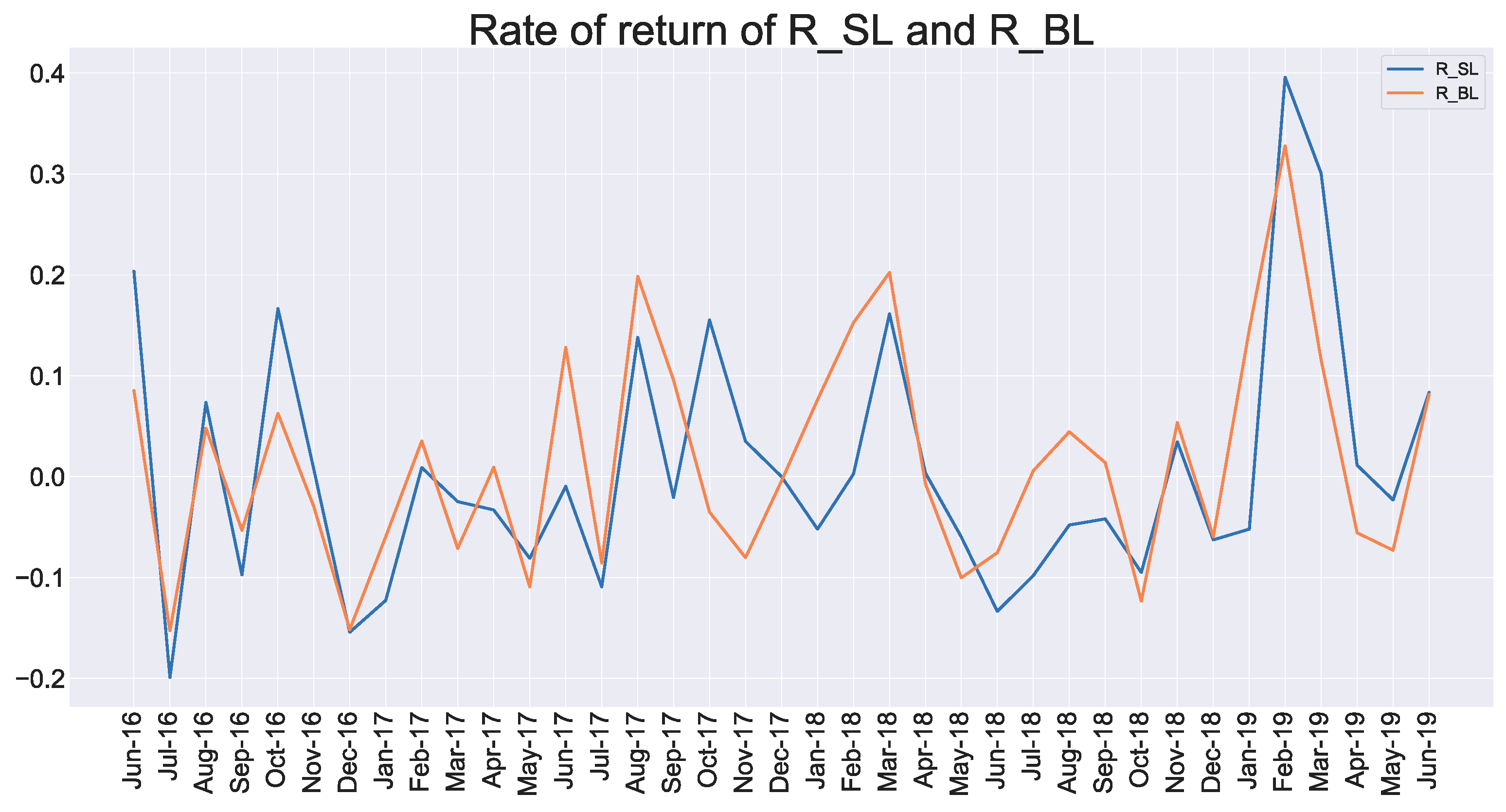
Subsequently, although all portfolios passed the F test, the independent variables in each portfolio should also be checked for the significance. There were two portfolios (S/L and B/L) under the FFTFM and one portfolio (B/L) under the four-factor model’s own independent variables that all passed the significance test.

6.2. Influence of Market Risk Premium Factor

The blockchain industry in China, including, but not limited to, the firms that take blockchain as FinTech, owns a positive relationship with the whole market environment. The coefficients of the independent variable market risk premium factor of all eight portfolios were more significant than 1, which implied that the investment portfolio could release the nonsystematic risk and contribute to the return of portfolios. The blockchain industry is an emerging market in China, and several update companies have begun to brace this technology recently, including the companies which use blockchain as FinTech. Along with the development of the blockchain industry, numerous investors are attracted by this industry and plan their investment in this as well. It causes higher volatility in return than the whole market.

6.3. The Non-Existence of Size Effect and Book-to-Market Ratio Effect in the Chinese Blockchain Industry

The size effect is that the return of small listed firms have significantly higher average returns than the large. Banz first found this effect and Fama and French verified the existence [5,55]. However, several researchers own opposite views about the size effect. Goyal and Welch concluded that this effect is caused by the deviation of sample selection rather than the size of the companies [56]. Dimon and Marsh believe that big companies could achieve a higher return than small firms [57]. Schwert claimed that the size effect is disappearing gradually. In this empirical research, the conclusion could be drawn that there is no size effect in the Chinese blockchain industry, which includes the firms using this technology as FinTech; portfolios with big companies bring a higher return [58].
The BM effect indicates that the return of the stocks has a positive relationship with the company’s market-to-book ratio. A higher book-to-market rate could bring out a higher stock return. Fama and French also believe the existence of the BM effect [5]. Chinese researchers drew a different conclusion about the BM effect in the Chinese securities market. Xu argued that there is a significant BM effect in the Chinese stock market [59]. Gu and Ding conducted an empirical study of the growth effect of China’s securities’ market and proved that the BM effect is non-existent [60]. According to the analysis of the Fama-French model above, the BM effect does not exist in the Chinese blockchain industry. Portfolios built by the low book-to-market ratio companies earn more returns than others.
There are various factors that affect the investment in the stock market and investors have been trying to obtain higher investment returns. Many scholars have also studied the effective factors in this filed and have proved that FFTFM can be applied to Western developed securities’ markets. Compared with these mature stock markets, the Chinese stock market has developed late. Therefore, whether the Chinese market can effectively meet the conditions for using the three-factor model has been under discussion. In recent years, with the continuous development of technologies, such as big data, methods for measuring investor sentiment have also advanced. The online forum is an important window for investors to express their sentiments. This article also took this factor into account to improve the model’s explanatory power. The empirical analysis of this article showed that there is no size effect in the Chinese blockchain industry, but there is a BM effect. Companies with more positive and optimistic concerns can bring higher returns to investors. These can help investors choose high-return companies in this field. We also need to admit that the method of sentiment analysis is still relatively simple, and the accuracy of text sentiment measurement needs to be improved. The extent to which the information in the online forum can affect investors’ decisions needs further research.

Author Contributions

Conceptualization, Z.J. and V.C.; methodology, Z.J., V.C., and H.L.; software, Z.J.; validation, V.C., R.V., and C.-H.R.H.; formal analysis, Z.J. and V.C.; investigation, Z.J. and H.L.; resources, V.C., H.L., R.V., and C.-H.R.H.; data curation, Z.J.; writing—original draft preparation, Z.J.; writing—review and editing, V.C., H.L., R.V., and C.-H.R.H.; visualization, Z.J.; supervision, V.C. and H.L.; project administration, V.C.; funding acquisition, Z.J., V.C., R.V., and C.-H.R.H. All authors have read and agreed to the published version of the manuscript.

Funding

This work was partially supported by VC Research (VCR 0000042) and the National Natural Science Foundation of China (Grant No. 61872084).

Conflicts of Interest

The authors declare no conflict of interest.

References

  1. Nakamoto, S. Bitcoin: A Peer-To-Peer Electronic Cash System. Available online: https://bitcoin.org/bitcoin.pdf (accessed on 1 September 2019).
  2. Mu, J. Opportunities, Challenges and Prospects of the Central Bank to Implement the Legal Digital Currency DCEP. Economist 2020, 31, 95–105. [Google Scholar]
  3. Mu, C.C.; Di, G.; Lv, Y.; Qian, Y.C.; Qing, S.D. Blockchain Research Group of Digital Currency Research Institute of PBC. China Financ. 2020, 70, 28–29. [Google Scholar]
  4. Markowitz, H.M. Portfolio selection. J. Financ. 1952, 7, 77–91. [Google Scholar]
  5. Fama, E.F.; French, K.R. The Cross-Section of Expected Stock Returns. J. Financ. 1992, 47, 427–465. [Google Scholar] [CrossRef]
  6. Fan, L.Z.; Yu, S.D. A Three-factor Model of Chinese Stock Market. J. Syst. Eng. 2002, 17, 537–546. [Google Scholar]
  7. Yang, X.; Chen, Z.H. Empirical Study on Three-factor Asset Pricing Model in Chinese Stock Market. Quant. Tech. Econ. 2003, 20, 137–141. [Google Scholar]
  8. Deng, C.R.; Ma, Y.K. Empirical Study on Three-factor Model in China’s Securities Market. Chin. J. Manag. 2005, 2, 591–596. [Google Scholar]
  9. Zhao, P.; Zhou, M. Research on the Applicability of Fama-French Three-Factor Model of Securities Industry in China’s A-share Market. Times Financ. 2018, 27, 156–157. [Google Scholar]
  10. Liu, T.J.; Zhu, J.Q.; Li, Y. An Empirical Analysis of the Applicability of Fama-French Three-factor Model in China’s Growth Enterprise Market. J. Jiaozuo Univ. 2013, 27, 64–66. [Google Scholar]
  11. You, D. An Empirical Study of Fama-French Three-Factor Model in China’s A-Share Real Estate Sector. Mod. Bus. Trade Ind. 2008, 20, 199–200. [Google Scholar]
  12. Li, Z.H.; Zhao, A.C. Research on the Return Rate Prediction of Electric Power Industry in Chinese Stock Market. J. Hebei Univ. Econ. Bus. (Compr. Ed.) 2018, 18, 34–39. [Google Scholar]
  13. Guo, Z.X. Fama-French three-factor model and five-factor model empirical test for A-shares steel companies. Hebei Enterp. 2019, 30, 33–36. [Google Scholar]
  14. Zhu, M. Empirical Test of Listed Bank Shares in China Based on Fama-French Three-Factor Model. Hebei Financ. 2019, 26, 17–21. [Google Scholar]
  15. Liu, W.Q.; Liu, X.X. Individual/institutional investor sentiment and stock returns: Study based on Shanghai A-share market. J. Manag. Sci. China 2014, 17, 70–87. [Google Scholar]
  16. Ba, S.S.; Zhu, H. Margin Trading, Short Selling, Investor Sentiment and Stock Market Volatility. Stud. Int. Financ. 2016, 32, 82–96. [Google Scholar]
  17. Liu, Y.C.F.; Zhang, Z.C. A Summary of Research on Investor Sentiment in Chinese Stock Market. China Econ. 2018, 32, 78–79. [Google Scholar]
  18. Fama, E.F.; French, K.R. Size, Value and Momentum in International Stock Returns. J. Financ. Econ. 2012, 10, 457–472. [Google Scholar] [CrossRef]
  19. Carhart, M.M. On persistence in mutual fund performance. J. Financ. 1997, 52, 57–82. [Google Scholar] [CrossRef]
  20. Xu, H.Y.; Xiong, C. Applicability of Carhart’s four-factor model in China’s stock market. Bus. Cult. 2009, 2, 128. [Google Scholar]
  21. Xue, S.Z.; Guan, X.Y. An Empirical Study on the Evaluation of Openended Fund Performance Based on “Four-Factors” Model. Financ. Teach. Res. 2011, 26, 63–65. [Google Scholar]
  22. Fama, E.F.; French, K.R. A five-factor asset pricing model. J. Financ. Econ. 2015, 116, 1–22. [Google Scholar] [CrossRef] [Green Version]
  23. Racicot, F.E.; Rentz, W.F.; Tessier, D.; Théoret, R. The Conditional Fama-French Model and Endogenous Illiquidity: A Robust Instrumental Variables Test. PLoS ONE 2019, 14, 1–26. [Google Scholar] [CrossRef]
  24. Racicot, F.E.; Rentz, W.F.; Kahl, A.L.; Mesly, O. Examining the dynamics of illiquidity risks within the phases of the business cycle. Borsa Istanb. Rev. 2019, 19, 117–131. [Google Scholar] [CrossRef]
  25. Sembiring, F.M. Three-Factor and Five-Factor Models: Implementation of Fama and French Model on Market Overreaction Conditions. J. Financ. Bank. Rev. (JFBR) 2018, 3, 77–83. [Google Scholar]
  26. Cox, S.; Britten, J. The Fama-French five-factor model: Evidence from the Johannesburg Stock Exchange. Invest. Anal. J. 2019, 48, 240–261. [Google Scholar] [CrossRef]
  27. Bangash, R.; Khan, F.; Jabeen, Z. Size, Value and Momentum in Pakistan Equity Market: Size and Liquidity Exposures. Glob. Soc. Sci. Rev. 2018, 3, 376–394. [Google Scholar] [CrossRef]
  28. Tian, L.H.; Wang, G.Y.; Zhang, W. Three-factor model pricing: How is China different from the United States? Stud. Int. Financ. 2014, 30, 37–45. [Google Scholar]
  29. Yang, J.H.; Fan, L.B. Global Market Integration: Fama-French Three-Factor Model Test in a Global Scenario. Technol. Econ. 2017, 36, 109–119. [Google Scholar]
  30. Feng, S.J.; Liu, Z. An Empirical Study of Three-factor Pricing Model in China Stock Market. Econ. Res. Guide 2018, 20, 145–148. [Google Scholar]
  31. Yan, X.; Pu, T. An Empirical Study of Fama-French Model in China’s Stock Market: A Case Study of Shanghai 50 Index. Times Financ. 2017, 11, 181–182. [Google Scholar]
  32. Yin, L.Y. An Empirical Study of the Impact of Investor Sentiment on Stock Returns: Based on the Fama-French Three-Factor Model. Friends Account. 2018, 6, 51–56. [Google Scholar]
  33. Hu, M.A.; Tu, X.P.; Zhu, D.Y. Is the Fama-French five-factor model more explanatory? Co-Oper. Econ. Sci. 2017, 10, 82–85. [Google Scholar]
  34. Yuan, J.Y.; Cong, Z. Research on the Stock Return of Hadaqi Listed Companies Based on Fama-French Three-Factor Model. J. Heilongjiang Inst. Technol. 2015, 29, 51–53. [Google Scholar]
  35. Cheng, S.Y.; Fang, H. Empirical Research on China’s Auto Sector Stock Yield Based on Fama-French Three-Factor Model. China Price 2019, 1, 71–73. [Google Scholar]
  36. Gou, D.N.; Wang, W.J. Empirical Test of China’s Listed Bank Shares Based on Fama-French Three-Factor Model. Stat. Decis. 2016, 21, 158–161. [Google Scholar]
  37. Baur, M.; Quintero, S.; Stevens, E. The 1986–88 stock market: Investor sentiment or fundamentals? Manag. Decis. Econ. 1995, 17, 319–329. [Google Scholar] [CrossRef]
  38. Mehra, R.; Sah, R. Mood fluctuations, projection bias, and volatility of equity prices. J. Econ. Dyn. Control 2002, 26, 869–887. [Google Scholar] [CrossRef]
  39. Brown, G.; Cliff, M. Investor Sentiment and Asset Valuation. SSRN Electron. J. 2001. [Google Scholar] [CrossRef] [Green Version]
  40. Cheng, K.; Liu, R. Research on the Interaction between Investor Sentiment and Stock Market. Shanghai Econ. Rev. 2005, 11, 88–95. [Google Scholar]
  41. Wang, C.F.; Zhao, W.; Fang, Z.M. Measure of IPO investor sentiment and its relationship with IPO price behavior. Syst. Eng. 2007, 7, 1–6. [Google Scholar]
  42. Wen, F.H.; Yang, X.; Gong, X.; Huang, C.X.; Yang, X.G. An Infectious Analysis of Sino-US Investor Sentiment in the Context of the Financial Crisis. Syst. Eng. Theory Pract. 2015, 35, 623–629. [Google Scholar]
  43. Tetlock, P. Giving Content to Investor Sentiment: The Role of Media in the Stock Market. J. Financ. 2007, 62, 1139–1168. [Google Scholar] [CrossRef]
  44. Chen, X.H.; Peng, W.L.; Tian, M.Y. Research on stock price and trading volume prediction based on investor sentiment. J. Syst. Sci. Math. Sci. 2016, 36, 2294–2306. [Google Scholar]
  45. Meng, X.J.; Meng, X.L.; Hu, Y. Research on Investor Sentiment Index Based on Text Mining and Baidu Index. Macroeconomics 2016, 1, 144–153. [Google Scholar]
  46. Luo, K.; Wang, C.F.; Fang, Z.M. Research on the Regionalization of Capital Asset Pricing under the Influence of Investors’ Emotion—Based on the Emotional Analysis of Stock Forum Posts. Oper. Res. Manag. Sci. 2017, 26, 129–136. [Google Scholar]
  47. Xu, T.Y. Research on the Impact of Investor Sentiment on the Stock Market in Social Media. Shanghai Manag. Sci. 2018, 40, 67–74. [Google Scholar]
  48. The number of blockchain companies has increased by 7159%. China Econ. Wkly. 2019, 11, 7.
  49. Fama, E.F.; French, K.R. Size and book-to-market factors in earnings and returns. J. Financ. 1995, 50, 131–155. [Google Scholar] [CrossRef]
  50. Wu, X.F.; Liu, Y.F.; Lei, M. An Empirical Analysis of Equity Premium in China’s Capital Market. Econ. Probl. 2007, 336, 85–88. [Google Scholar]
  51. Qu, Z.X. Research on Value Evaluation Method of Non-tradable Shares of Listed Companies. Business 2012, 9, 48. [Google Scholar]
  52. Zhang, Z.C.; Liu, Y.C.F. The Construction and Effectiveness Test of Investor Sentiment Index in my country’s Stock Market. Commer. Times 2018, 7, 156–158. [Google Scholar]
  53. Antweiler, W.; Frank, M.Z. Is all that talk just noise? the information content of internet stock message boards. J. Financ. 2004, 59, 1259–1294. [Google Scholar] [CrossRef]
  54. Bu, H.; Xie, Z.; Li, J.H.; Wu, J.J. The Impact of Investor Sentiment Based on Stock Evaluation on the Stock Market. J. Manag. Sci. China 2018, 21, 86–101. [Google Scholar]
  55. Banz, R.W. The Relationship between Return and Market Value of Common Stocks. J. Financ. Econ. 1981, 9, 3–18. [Google Scholar] [CrossRef] [Green Version]
  56. Goyal, A.; Welch, I. Predicting the Equity Premium; manuscript; Yale University: New Haven, CT, USA, 1999. [Google Scholar]
  57. Dimson, E.; Marsh, P. Murphy’s Law and Market Anomalies. J. Portf. Manag. 1998, 25, 53–69. [Google Scholar] [CrossRef]
  58. Schwert, G.W. Anomalies and market efficiency. In Handbook of the Economics of Finance; Elsevier: Amsterdam, The Netherlands, 2003; pp. 939–974. [Google Scholar]
  59. Xu, Z.H. An Empirical Analysis of China’s Stock Market Scale Effect and Book-to-Market Ratio Effect. J. Financ. Dev. Res. 2011, 11, 75–78. [Google Scholar]
  60. Gu, J.; Ding, Y. An Empirical Study on the Growth Effect of China’s Securities Market. Econ. Rev. 2003, 2, 101–105. [Google Scholar]
Figure 1. Tendencies of return rate of four portfolios and market risk factor.
Sustainability 12 05170 g001
Figure 2. The return of portfolio S/L (Small-and-Low) and B/L (Big-and-Low).
Sustainability 12 05170 g002
Figure 3. The return of portfolio S/H (Small-and-High) and B/H (Big-and-High).
Sustainability 12 05170 g003
Table 1. Return of each portfolio’s descriptive analysis.
Test FocusR_SLR_SHR_BLR_BHRm-RfSMBHML
count37373737373737
mean0.007166−0.019920.01505−0.01115−0.12047−0.00833−0.02664
std0.1248660.0912180.1085230.0813830.0447230.0498320.05708
min−0.19904−0.14461−0.15265−0.12005−0.20996−0.11855−0.1435
25%−0.06269−0.07561−0.07093−0.08007−0.14663−0.03881−0.06217
50%−0.02073−0.042070.005983−0.01998−0.11772−0.00401−0.0235
75%0.0350040.0175230.0816350.0212−0.093860.0169860.013356
max0.3959680.2788530.3278640.2458980.0246080.1017690.089053
Table 2. Correlation among parameters and portfolios’ return.
Test Variables-rm-rfSMBHMLR_SLR_SHR_BLR_BH
rm-rf10.19−0.10.560.680.540.67
SMB0.191−0.0820.540.34−0.130.16
HML−0.1−0.0821−0.59−0.12−0.59−0.16
R_SL0.560.54−0.5910.790.720.79
R_SH0.680.34−0.120.7910.750.92
R_BL0.54−0.13−0.590.720.7510.78
R_BH0.670.16−0.160.790.920.781
Table 3. Results of the augmented Dickey–Fuller (ADF) test.
Portfolios1% Critical Value5% Critical Value10% Critical Valuet-Valuep-Value
S/L (S/L including sentiment)−3.6267−2.9460−2.6117−5.41650.000
S/H (S/H including sentiment)−3.6327−2.9485−2.6130−5.02230.000
B/L (B/L including sentiment)−3.6392−2.9512−2.6144−4.37140.000
B/H (B/H including sentiment)−3.6327−2.9485−2.6130−5.21750.000
Table 4. Results of the autocorrelation test.
Test Variables and FocusDurbin-Watson StatisticDurbin-Watson Critical Value (Upper)chi2Prob > chi2
S/L2.3561.6551.3420.2467
S/H2.0821.6550.1520.6970
B/L2.0821.6550.1520.6970
B/H2.3561.6551.3420.2467
S/L (add sentiment)2.3301.7231.1640.2807
S/H (add sentiment)1.9961.7230.0140.9057
B/L (add sentiment)2.1081.7230.1800.6712
B/H (add sentiment)2.1291.7230.1810.6703
Table 5. Variance inflation factor (VIF) results.
Three-Factor Model Collinearity Statistics
ToleranceVIF
S/L, S/H, B/L, B/H(Constant)
Rm-Rf0.8891.124
SMB0.951.053
HML0.9411.063
Four-factor model Collinearity Statistics
ToleranceVIF
S/L (Constant)
VAR000020.8891.124
SMB0.951.053
HML0.9411.063
S_SL0.8821.133
S/H(Constant)
VAR000020.9511.052
SMB0.9461.058
HML0.9821.018
S_SH0.9731.027
B/L(Constant)
VAR000020.9571.045
SMB0.9021.109
HML0.7421.347
S_BL0.7271.375
B/H(Constant)
VAR000020.9561.046
SMB0.9331.072
HML0.9761.024
S_BH0.961.041
Table 6. Results of the White test.
Test Variables and Focuschi2Prob > chi2
S/L9.700.3751
S/H16.500.0572
B/L16.500.0572
B/H9.700.3751
S/L (add sentiment)12.780.5438
S/H (add sentiment)24.330.0518
B/L (add sentiment)21.670.0856
B/H (add sentiment)17.260.2426
Table 7. Goodness-of-fit test of traditional FFTFM (Fama-French Three-Factor Model).
S/LS/HB/LB/H
R 2 0.7700.5090.6530.458
R ¯ 2 0.7490.4640.6210.409
Durbin-Watson statistic2.3562.0822.0822.356
Table 8. Results of F test.
S/LS/HB/LB/H
F test (3,33)36.8111.3820.689.309
Prob (F)0.00000.00000.00000.000132
Table 9. Results of t-test.
S/LS/HB/LB/H
β i 1.19391.29421.29421.1939
t-test(−5.009) ***(5.086) ***(5.086) ***(5.009) ***
s i 1.04960.3943−0.60570.0496
t-test(4.916) ***(1.730) *(−2.657) **(0.232)
h i −1.1229−0.0612−1.0612−0.1229
t-test(−6.102) ***(−0.312)(−5.402) ***(−0.668)
α i 0.00570.01360.01360.0057
t-test(0.184)(0.409)(0.409)(0.184)
*** Indicates the coefficient passing the t-test at the 1% level. ** Indicates the coefficient passing the t-test at the 5% level. * Indicates the coefficient passing the t-test at the 10% level.
Table 10. The results of goodness of fit and F test of four-factor pricing model.
Test FocusS/LS/HB/LB/H
R 2 0.7710.5290.6890.514
R ¯ 2 0.7430.470.650.453
F test(3,32)278.97617.78.447
Prob(F)0.00000.00000.00000.0000
Table 11. Results of regression of four-factor pricing model.
Test FocusS/LS/HB/LB/H
α i 0.0060.01260.0075−0.012
t-test0.1890.3830.235−0.382
β i 1.22451.31741.2891.1852
t-test4.894 ***5.19 ***5.267 ***5.166 ***
s i 1.060.4275−0.49840.1167
t-test4.878 ***1.871 *−2.203 **0.56
h i −1.1042−0.0487−0.8535−0.155
t-test−5.793 ***−0.249−3.922 ***−0.872
s e n t i 0.03510.10540.24690.1493
t-test0.4611.1721.922 *1.906 *
*** Indicates the coefficient passing the t-test at the 1% level. ** Indicates the coefficient passing the t-test at the 5% level. * Indicates the coefficient passing the t-test at the 10% level.

