Formation Factors and Effects on Common Property Resource Conservation of Community Farms

Abstract

In recent decades, there has been a global debate over who should manage common property resources (CPRs) related to agriculture. Because rational and efficient farmers only work farmland with good conditions or leave for other industries, in areas where production conditions are poor, local resources that were once collectively maintained are no longer managed. The Japanese government has positioned community farms (CFs) as an important player in local agriculture and has been striving to develop them. This study clarifies whether the formation and development of these CFs are functioning effectively for the conservation of local resources. Specifically, we use the propensity score matching method to measure the average treatment effect of CF formation and development on CPR conservation activities and the prevention of cultivation abandonment. In particular, this study tests the hypothesis that farmers are reluctant to develop CFs extensively because their effects on CPR conservation are uncertain. The results show that at the early stage, the formation of CFs has a significantly positive effect on the promotion of CPR conservation, but its wide-area development is counterproductive to CPR management, suggesting that resourceful support is needed according to local conditions.

1. Introduction

Farmers take on various roles depending on the country and geographical conditions, including maintaining local economies and managing common property resources (CPRs) through community-based collaborative activities, as well as agricultural production [1,2]. In agriculture, the management of local resources has long been implemented as a collective activity of local members; thus, securing agricultural management entities that play a role in communities is indispensable to sustain local resource management [3]. However, such CPRs have been developed over a long period, and their benefits are dispersed both spatially and temporally, making them difficult to evaluate [4].

In countries where the comparative advantage of agriculture has been declining for a long time, it is urgent to secure an agricultural labor force to prevent a decline in the national food self-sufficiency rate [5]. Particularly in Japan, land-intensive agriculture, such as paddy cultivation, is declining rapidly. One of the most important issues in Japanese agricultural policy is how to secure and develop leaders and labor to maintain the spread of rice fields across the country [6]. In fact, in Japan, the abandoned cultivated area has increased remarkably, and the abandoned cultivated land rate has increased from 2.7% in 1975 to 10.6% in 2010. Especially in disadvantaged areas, it exceeded 14% in 2010 [7]. In Japan, the disadvantaged areas, called the hilly and mountainous areas, are generally defined by the slope of farmland, percentage of forest and mountain, and population density. Since these areas account for about 40% of farmland and 35% of agricultural output value, conservation of the farmland is an important issue for food security in Japan [7]. Under such circumstances, the Basic Plan for Food, Agriculture and Rural Areas issued by Japan’s Ministry of Agriculture, Forestry and Fisheries (MAFF) designates a few types of agricultural management entities as core players responsible for future agriculture, including community farms (CFs), as well as large-scale individual farmers and agricultural corporations [8].

The term “community farm“ has various meanings depending on different times and regions. In former communist countries, communal (collective) farms were forced to form under the leadership of the central government [9,10], which is quite different from what we target. Our target is a farm that is jointly managed as a democratic economic entity by farmers within a community. In recent years, mainly in Western Europe, community farms have been referred to as farms that offer a variety of values, such as tourism and organic food [11,12]. These farms are emerging as conceptual entities as part of the community supported agriculture, which supports the food supply chain and people’s new values in the area. On the other hand, in monsoon Asia, communities play an important role as a group for collective action. This is because water management is crucial for producing rice, the staple food in Asia [13,14]. In addition, since farmlands are small and dispersed, communication and coordination within the community is required to make decisions on how to distribute water [15]. Therefore, irrigation facilities are generally managed by many community members [3]. Further, group farms, as members of the community, are inevitably required to cooperate with individual farmers and farmland lessors to manage water and conserve CPRs. The higher the group participation rate, the lower the transaction costs related to collective action, and so the community can efficiently conserve CPRs [3,16,17]. From the viewpoint of agricultural productivity, Tada and Ito [6] showed that since farmers’ groups such as CFs share agricultural machinery with other farmers, their technical efficiency is higher than that of large-scale individual farmers; however, total productivity, especially land productivity, is reported to be inferior to that of large-scale individual farmers [6].

In Japan, “community-based farm cooperatives”—or simply CFs—“consist of farming households in certain regions that have developed relations through local communities or other geographical bases. Cooperative member households conduct joint agricultural production. These cooperatives’ … operations range from the aggregation of diverted paddy fields and the communal use of communally purchased machines to joint production and sales in which farming leaders play a central role” [18]. Community farms require efficient business management and are also expected to play a role as local resource managers. Although in flat areas large-scale family farms can still manage efficiently, CFs are expected to play a major role in disadvantaged areas. Therefore, the promotion of CF formation by the Japanese government is highly policy-oriented [19]. Agricultural corporations and individual farmers who manage large-scale operations tend to leave disadvantaged (hilly and mountainous) areas, so CFs are essential agricultural management entities that protect farmland, local resources, and agriculture in disadvantaged areas. However, despite policy efforts, many problems still exist in disadvantaged areas, such as insufficient management of irrigation facilities and reservoirs, as well as abandoned farmland. Unless CFs take over the collective management of CPRs that individual farmers once ran collectively, CPRs will be hindered. Furthermore, in Japan’s rural areas, depopulation and the aging of the people are rapidly progressing and economic conditions are deteriorating significantly; therefore, CFs also need to play a role as economic agents supporting the local economy [20].

The conservation of CPRs can be generally considered a collective action of community residents and farmers. Ostrom [21] discusses structural variables that affect the likelihood of participation in collective actions, showing group size as one of the key factors. This proposition, which has been discussed for more than 50 years, has its roots in the claim by Olson [22] that the greater the group size, the lower the probability that the public good will be achieved (group-size paradox). In general, group size also has a positive effect on collective action, as it strengthens the complementarity of the organization and expands the available resources for collective action [23]. The most basic reason for this paradox is possibly that as the group size increases, the probability of successful freeriding increases, and so do the transaction costs of the agreement process [21]. Obviously, the larger the group size, the higher the monitoring costs for managing CPRs. If the costs cannot be secured or firmly set, it is easier for CF members to avoid the burden of conservation activities. Meanwhile, the effect of transaction costs is subtle. As organizations grow, the costs of finding different business partners decrease, while the costs of communication and conflict resolution between communities increase. Therefore, the effect of group size is mixed.

Agrawal [24] argues that small groups may not be able to protect their resources due to the lack of capacity to obtain a surplus for effective resource management, whereas the broadening of the group impedes the formation of an organization that can manage and conserve CPRs under external environmental conditions, indicating a non-linear relationship between group size and the probability of resource conservation. Baland and Platteau [25] state that small groups can create rules tailored to local conditions and can adjust procedures and rules as conditions change. These studies imply that the effect of group size on resource management is mixed. Assuming that the population density of a community in a region is uniform, the expansion of the area of activity means an increase in the number of participants involved, so the CF development that we consider applies to this context. As later shown, the formation of CFs has become quite prevalent in Japan, but their development has not progressed as the government expected. We believe that the reason farmers are hesitant to develop CFs is that they anticipate insufficient effects. That is, we test the hypothesis that the spatial development of CFs impairs the conservation of CPRs. Therefore, this study contributes to the discussion on the conditions—particularly group size—of CFs that adequately preserve CPRs [21,22,23,24,25].

In our analysis, we examine how the formation and development of CFs contribute to local resource management, the prevention of abandoned farmland, and the revitalization of the local agricultural economy. Specifically, this study sets the following two goals. First, we identify, using a regression analysis, the drivers and barriers that affect the formation of CFs and their development into multi-CF partnership organizations (PCFs). Although CFs and PCFs have different sizes, they are essentially the same from an institutional point of view. It should be noted that Japanese farmers, especially rice farmers, have historically worked together in local communities to carry out collective actions for the management of irrigation facilities, which implies that it is extremely difficult for them to manage paddy agriculture without participating in collective action. Therefore, to develop a CF into a PCF, first, the permission of the majority of community members is essential.

For this analysis, we assume three stages of CF development: one without community farming (NCF), one in which a CF is established in each community (CF), and a stage in which CF partnerships are developed (PCF). Next, we examine how CFs and PCFs contribute to the conservation and management of CPRs, the prevention of farmland abandonment, and the performance of local agriculture. In this analysis, we consider the formation of CFs or PCFs as a “treatment” to estimate their effects through a causal inference framework. CFs and PCFs do not occur randomly because their formation is determined voluntarily according to the local situation. Therefore, if the difference in performance is measured simply by the existence (or not) of a CF or PCF, the treatment effect includes selection bias. That is, to estimate these true effects, it is necessary to impute counterfactuals and compare them with real data. We estimate the causal effects using the propensity score matching (PSM) method, which has recently been adapted for the social sciences [26].

CFs were formed relatively early in the Kinki region of Japan, which is the focus area of our research [19]. However, although the organization ratio of CFs is high in our study area, it tends to be extremely low for PCFs. We focus on filling this paradoxical gap, addressing empirical challenges. Because farmers may believe that they are unlikely to conserve CPRs and gain economic benefits or that their motivation for farming will be distorted by developing CFs into PCFs, it is likely that they will be hesitant to form a PCF as a rational action. Testing the hypothesis that farmers are reluctant to develop CFs extensively because their effects on CPR conservation are uncertain is one of the most important purposes of this study.

2. Methodologies and Data

2.1. Coding Method for Community Farms

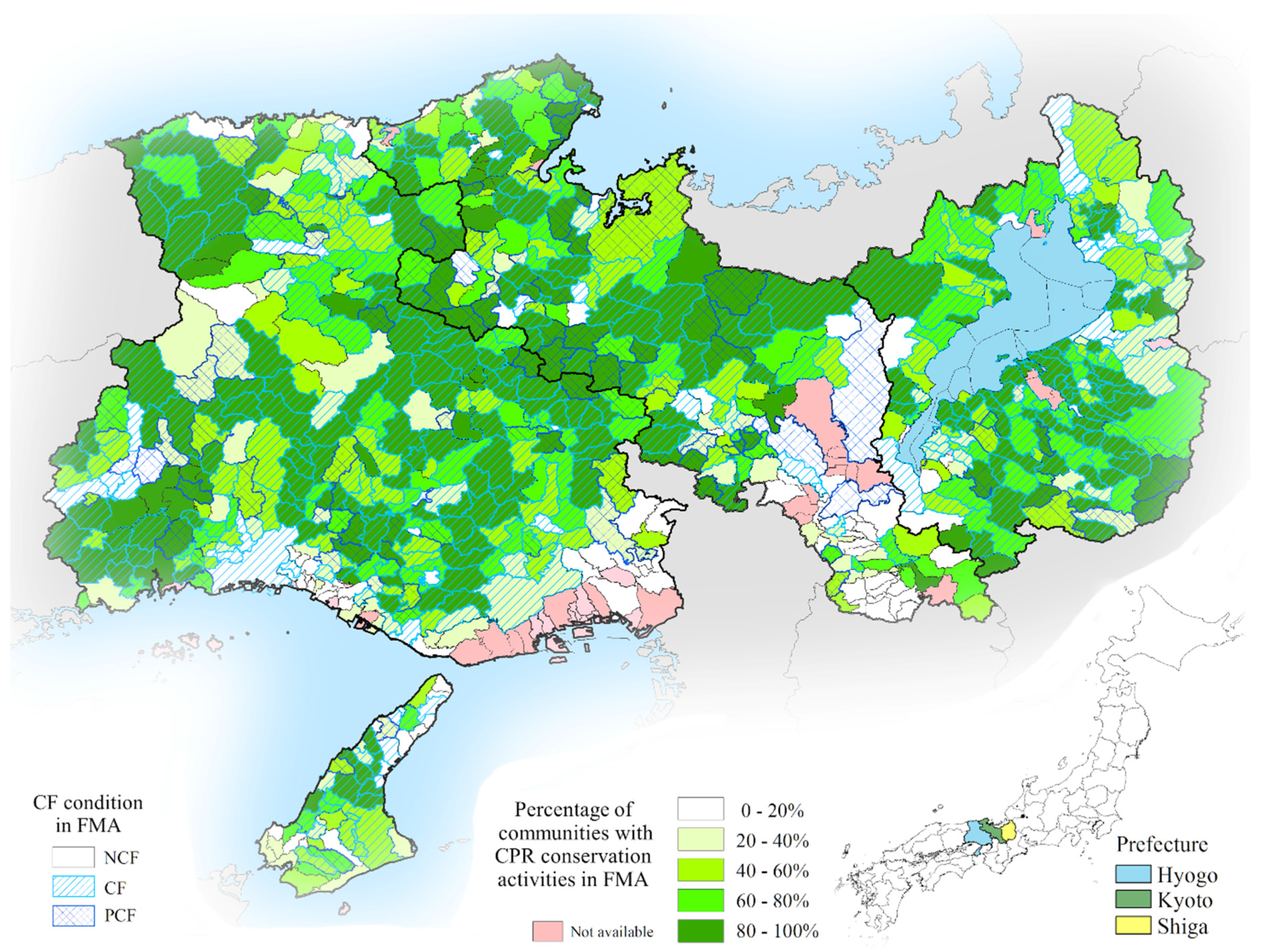
In Japan, CFs emerged in the 1980s as agricultural management entities that efficiently and collectively use farmland and agricultural machinery [27]. They were formed due to a shortage of agricultural labor in areas where farming per household was low and urbanization created plentiful part-time jobs [20]. In the 1990s, when domestic agricultural prices declined due to trade liberalization, the profits of individual family farms declined, prompting the further establishment of CFs [28,29]. Since the 2000s, they have been established to meet the requirements of direct payment policies [30]. Under such circumstances, MAFF has encouraged local governments to develop CFs into corporate organizations that can secure more sustainable management and credit [31]. In recent years, there has been a rise in the number of CFs that have developed and expanded beyond local communities [32,33,34,35]. Since 2015, MAFF has been providing financial support for agreements between CFs in areas where depopulation and aging make it difficult to secure human resources for CFs [19]. Under these circumstances, the number of CFs has increased from 10,063 in 2005 to 14,832 in 2020 (out of 138,256 total agricultural communities). Regarding the cultivated area per CF (including PCFs), CFs with less than 10 ha had the highest ratio of 27.2%, followed by those with 10–20 ha with 23.2% and with 30–50 ha with 17.8% [36].

This leads us to examine how the development of CFs contributes to CPR conservation, farmland conservation, and farmers’ economic performance. To this end, it is important to code NCFs, CFs, and PCFs, which represent the development stages of CFs, within each area as ordinal categorical data. To do this, we used data from the Survey on Community-based Farm Cooperatives (SCFC) conducted by MAFF [37]. The SCFC includes data such as whether a CF exists in each community, as well as agriculture-related activities, which are also aggregated at the former municipal level. The former municipal level area (FMA) is larger than the community level but smaller than current municipalities. Because these areas mirror the elementary school districts and the active areas of the Japan Agricultural Cooperative (called “JA”) branches, they constitute the basic economic and living infrastructure for farmers. The reason for using FMA-based data is that the PCFs are generally formed in a larger area than the community, so we need to code them in the FMA to identify their existence (in statistical surveys, a PCF also can only be counted and identified as a CF).

SCFC data count the number of CF organizations in each community and also in the FMA. However, the aggregate value at the community level is not always the same as the value at the FMA level in the SCFC. For example, suppose that two adjacent communities constitute an FMA and that these two CFs have a partnership agreement across the communities. Each community has a CF, so the total aggregated number of organizations in the FMA is two. However, at the FMA level in the SCFC, it is counted as one CF (PCF in this case). Assuming that our aggregated number of CFs at the FMA level is $\alpha$ and that the number of CFs at the FMA level in the SCFC data is $\beta$, we code the condition of each FMA as follows:

$$\begin{gathered} T=0 if \alpha =0 \left(and \beta =0\right), \\ T=1 if 0<\beta =\alpha , \\ T=2 if 0<\beta <\alpha . \end{gathered}$$

Here, $T$ is a categorical variable: $T=0$ when no CF exists in the FMA (NCF), $T=1$ when only CFs exist (CF), and $T=2$ when any PCF exists. We assume that a community farm develops in this order. In the PSM analysis, when estimating the treatment effect of a CF, the analysis is performed with $T=1,2$ as the treatment group and $T=0$ as the control group. In the case of the treatment effect of a PCF, after deleting the data of $T=0$, the PSM method is applied using $T=2$ as the treatment group and $T=1$ as the control group. Since the SCFC is a complete survey, the control group that is a candidate for counterfactuals is composed of all FMAs other than the FMAs identified as treatment.

2.2. Study Area

Our targeted study area includes the Hyogo, Kyoto, and Shiga prefectures, which are located in the Kinki district, the central part of Honshu Island, Japan (Figure 1). This area encompasses many communities bordering the sea, both to the north and south, and is therefore geographically and climatically diverse, with a wide variety of agriculture. In addition, these areas are adjacent to the megalopolis called the Keihanshin zone, which is the second most populated area in Japan after Tokyo. Therefore, agriculture in these three prefectures plays an important role in providing food to urban residents. Shiga has the largest lake in Japan, Lake Biwa, which is a vital source of water resources for the surrounding area. The middle and southern parts of the study area are characterized by relatively flat land and little rain. Thus, irrigation ponds have long been used to supply water resources [38]. Rice production accounts for 33.6% of the Kinki region′s total agricultural production (total agricultural production: 301.8 billion yen; rice production: 101.5 billion yen), which is significantly higher than that of the whole country (18.8%) [39,40]. Therefore, the management of water resources in this area is extremely important because the agriculture there depends heavily on rice.

The Japanese government has positioned CFs as important players in the country’s future agriculture and expects them to not only function as efficient economic agents but also manage CPRs and maintain farmland. Figure 2 shows the percentage of communities with CFs and PCFs in all of Japan, the Kinki area, and the study area. Our study area has an extremely high CF formation ratio compared to the national level (Hyogo ranks seventh, Kyoto eighth, and Shiga first among 47 prefectures nationwide). The results may reflect the high paddy field rates and the need for water resource management in these areas, as well as the high percentage of part-time farmers due to their proximity to urban areas. Surprisingly, however, the PCF formation ratio is very low in the study area. Shiga has the lowest PCF ratio in Japan, followed by Hyogo (Kyoto is the twelfth lowest). Thus, the reason why the CF and PCF formation ratios show opposite tendencies is an important empirical question.

Figure 1 also shows the conditions of CFs and PCFs and the percentage of communities that manage CPRs in FMAs. There are some FMAs without CFs and PCFs in the coastal area near the city and the mountainous area in the center, but sysptematic regional trends cannot be observed in other areas. In addition, the percentage of communities that manage CPRs seems to be somewhat positively correlated with CFs, but this correlation is not clear. This study examines this causal relationship from the viewpoint of the treatment effect of CFs and PCFs.

2.3. Propensity Score Matching (PSM)

To examine the consequences of CF and PCF formation, we use the PSM method. The PSM method is a technique for estimating the average treatment effect (ATE) for a certain treatment. The formation of CFs and PCFs (hereinafter also referred to as treatments) is not naturally determined exogenously or randomly but is a voluntary decision made by local farmers. If a randomized controlled trial is possible, the ATE can be easily estimated by comparing outcomes between the treatment and control groups. However, in the social sciences, it is usually impossible to randomize experimental treatments due to cost and ethical aspects, so it is necessary to use observational data. The formation of CFs in this study is also not randomized, and the simple difference of the outcomes between the treated and control groups includes selection bias. The PSM method estimates the true ATE by complementing counterfactuals (control groups) for observation data [25]. Causal inference methods include techniques such as instrumental variables and difference-in-difference. However, these methods cannot be used here because there is no appropriate instrumental variable, and the SCFC only has data based on the communities in 2015. As discussed in a later section, the PSM method offers advantage; it can detect the heterogeneous effect of the treatment and so can more easily perform rich analysis than other methods [41].

The treatment in this study means that a CF or PCF is formed in a specific area. If the outcome of the treatment group is $Y_1$, the outcome of the control group is $Y_0$, and the treatment is randomized, the ATE can be expressed by the following equation:

$$ATE=E\left[Y_1\right]-E\left[Y_0\right].$$

(1)

However, our treatments of CFs and PCFs are not determined randomly because they are affected by various attributes of the community such as size, number of young farmers and successors, local social capital, and farmland liquidity. Furthermore, if those attributes also affect each outcome, they become confounders, and the ATE calculated by Equation (1) thus has a selection bias. To overcome this, we apply Rubin’s causal inference model [42]. Specifically, given covariates $\mathit{X}$ as confounding factors and treatment variables indicating the presence or absence of treatment as $T$ ($T=1$ if treated, 0 otherwise), if the following formula is satisfied, Equation (1) measures an appropriate causal effect.

$$\left(Y_1,Y_0\right)\perp T|\mathit{X}$$

(2)

This is referred to as the conditional independence assumption (CIA), but because $\mathit{X}$ has many factors, it is procedurally difficult to guarantee each independence (known as the “curse of dimensionality”). The solution to this problem is the PSM method, which reduces the multidimensional $\mathit{X}$ to the one-dimensional probability of the treatment, that is, the propensity score (PS). Using the PS, the PSM method ensures the independence of the treatment and outcome as in the following equation:

$$\left(Y_1,Y_0\right)\perp T|P\left(\mathit{X}\right).$$

(3)

The probability $P\left(\mathit{X}\right)$ of the treatment can be estimated as a predicted value when $T$ is regressed to $\mathit{X}$. We use a general binary probit model for this regression. Observations are matched by the estimated PSs, and counterfactuals for both the treatment and control groups are imputed. We use a one-to-one nearest neighbor matching algorithm for this procedure [43]. For testing the difference of outcomes between these two groups (i.e., ATE), we use a simple t-test.

To check the robustness of these results, an estimation using an inverse probability treatment weighting (IPTW) method is also performed [44]. In the IPTW method, if the correct PSs are estimated and the strongly ignorable treatment assignment condition is satisfied, it is possible to estimate the ATE without bias. That is, the ATE can be represented by the following equation, in which n is the number of samples.

$$AT{E}^{IPTW}=\frac{1}{n}{\displaystyle \sum }_{i=1}^n\frac{T_i{Y}_i}{P\left({\mathit{X}}_i\right)}-\frac{1}{n}{\displaystyle \sum }_{i=1}^n\frac{(1-T_i)Y_i}{1-P\left({\mathit{X}}_i\right)}$$

(4)

The estimate of the ATE can be calculated as the coefficient of the treatment dummy through a general regression analysis using all observed outcomes and weighting the inverse probabilities of the PS [41]. For estimation of PSM, R 3.6.1 and the R package “Matching” (ver. 4.9–7) were used [45].

2.4. Data

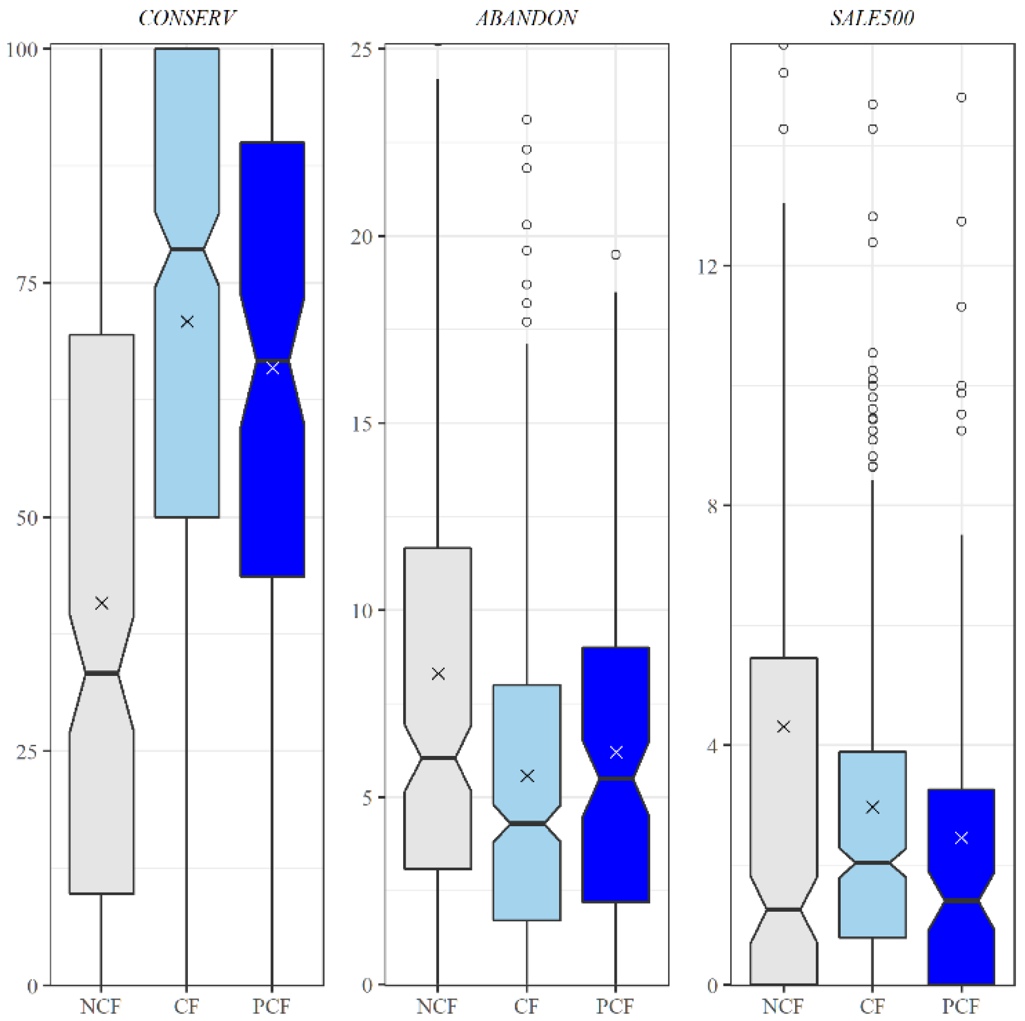
2.4.1. Outcomes of Causal Inference

All data except the SCFC data are compiled primarily from agricultural census surveys [46]. These data are tabulated for various attributes of farmers at the municipal, FMA, and community levels, of which we use FMA-level data.

Our outcomes using the PSM method include the percentage of communities conducting CPR conservation activities (CONSERV), the rate of abandoned farmland (ABANDON), and the percentage of agricultural management entities that earn more than 5 million yen in agricultural sales (SALE500). As noted in Section 2.2, conducting CPR conservation activities is the most important role governments expect of CFs. Therefore, CONSERV is a particularly important outcome in this study. In hilly and mountainous areas, MAFF expects CFs to play a role in preventing abandoned farmland. Therefore, a decrease of ABANDON in an FMA with a CF means that the CF is contributing to policy objectives. SALE500, the proportion of large-scale farms, is a proxy for the vitality of the local agriculture. The average income in Japan is about five million yen, and without enough agricultural sales, full-time employees cannot be hired, so this value was used as the threshold [47]. In 2015, there were 200,000 management entities nationwide that satisfied this condition (more than 5 million yen in sales), accounting for 13.9% of all farmers [39]. If a CF is formed and performs well economically, SALE500 will improve. However, if business conditions after a scale expansion are expected to deteriorate, farmers may be hesitant to form CFs and PCFs. Therefore, SALE500 is also a useful indicator for analyzing the economic motives for developing CFs into PCFs.

Figure 3 compares the distribution of these three outcomes according to community conditions. For CONSERV, a large positive difference can be confirmed between NCFs and CFs, whereas a negative difference is observed between CFs and PCFs. Similarly, for ABANDON, the formation of CFs has a positive effect on suppressing the occurrence of abandoned farmland, whereas PCFs do not appear to have this effect. In addition, for SALE500, the formation of CFs appears to impede the emergence of large business entities. The notches in Figure 3 represent the 95% confidence interval of the median. In the case of CONSERV, there is a significant positive difference between NCFs and CFs and a significant negative difference between CFs and PCFs. For ABANDON, there is a significant negative difference between NCFs and CFs (indicating improvement). However, these results show simple differences between groups and are not true causal effects of treatment (due to CF or PCF formation) because confounding factors that affect both treatment and outcome may cause selection bias.

2.4.2. Covariates for Probit Estimation

The covariates for calculating PSs are shown in

Table 1. Descriptive stats by CF conditions.

	Whole Data		NCF		CF		PCF
	Mean	SD	Mean	SD	Mean	SD	Mean	SD
Number of communities in old village: NCOM	10.16	8.56	7.60	5.61	10.82	8.40	13.50	12.26
Number of farm households per community (10 households): FHH	1.53	0.99	1.27	1.07	1.70	0.96	1.43	0.78
Percentage of part-time farm households in old village (%): PFARM	0.59	0.12	0.56	0.16	0.59	0.10	0.61	0.10
Percentage of non-farm households in old village (%): NFARM	70.55	29.77	76.18	24.17	68.60	33.35	66.08	24.43
Cultivated area per community: AAREA	0.99	0.52	0.89	0.58	1.06	0.49	0.94	0.51
Percentage of rented-out farmland in old village (%): RENTOUT	7.24	5.47	5.85	5.10	7.92	5.34	7.73	6.17
Percentage of farmers with cultivated areas of more than 5 ha (%): OV5	1.59	2.87	1.28	3.69	1.86	2.51	1.25	1.90
Percentage of farmers with successor (%): SUCCESS	7.26	7.50	10.28	9.73	6.09	6.17	5.43	4.30
Percentage of farmers under 40 years of age (%): AGEU40	16.43	4.35	16.36	4.78	16.79	3.93	15.29	4.71
Percentage of farmers with rice comprising the majority of sales (%): RICE	79.91	21.70	69.41	29.45	85.54	14.64	80.91	16.01
Number of meetings per community (10 meetings): MEET	1.40	0.81	1.03	0.78	1.60	0.80	1.43	0.60
Percentage of communities receiving MPS: MPS	0.19	0.35	0.15	0.35	0.20	0.33	0.24	0.41
Percentage of communities receiving DPHM: DPHM	0.70	0.64	0.42	0.64	0.89	0.60	0.67	0.49
Percentage of communities designated as depopulated: DEPOP	0.22	0.41	0.21	0.40	0.21	0.40	0.26	0.44
A dummy of some slope of cultivated area: SLOPE	34.96	35.18	28.91	33.54	37.02	35.45	40.13	36.15
Percentage of communities located in hilly and mountainous areas (%): HMA	0.57	0.50	0.51	0.50	0.58	0.49	0.68	0.47
Percentage of communities located in Hyogo pref. (%): HYOGO	0.50	0.50	0.50	0.50	0.51	0.50	0.45	0.50
Percentage of communities located in Kyoto pref. (%): KYOTO	0.27	0.44	0.37	0.48	0.17	0.37	0.42	0.50
Percentage of communities located in Shiga pref. (%): SHIGA	0.23	0.42	0.13	0.33	0.32	0.47	0.13	0.34
N	769		250		407		112

. Many possible factors influence the formation of CFs and PCFs. These variables were selected following previous studies analyzing community decision-making [3,48]. NCOM indicates the number of communities in an FMA, controlling for the FMA size effect. FHH is the average number of farms per FMA. When a community makes a collective decision, there may be an optimal number of members in the community [49]. Therefore, in our regression, we add the FHH squared term to the model. PFARM and NFARM represent the percentage of part-time farmers and non-farm farmers, respectively. If many of the households are less dependent on agriculture, activities conserving CPRs can be burdensome for them, which consequently may promote the formation of CFs and PCFs. However, this effect is still unclear because transaction costs for collective activities may be high. AAREA is the average farm size variable in an FMA, controlling for spatial and managerial farm size factors.

RENTOUT, which represents the percentage of farmland rented, indicates the degree of farmland liquidity in the area. In areas where the liquidity of agricultural land is high, CFs may be more likely to be formed due to lower transaction costs for consolidating land. OV5 is the proportion of farmers with more than 5 ha of farmland, which are relatively large agricultural management entities in Japan. These entities could be competitors to CFs, which could negatively affect the formation and development of CFs.

AGEU40 and SUCCESS represent the percentage of farmers under the age of 40 and agricultural management entities with successors, respectively. Although young farmers and successors may develop their own businesses, they may be candidates for CF and PCF leaders, meaning that these effects are mixed. RICE is a variable that indicates rice dependence, which is used to test the hypothesis that areas with many rice farms require CFs to maintain paddy fields and irrigation facilities. MEET, the number of meetings in the community, is a proxy variable of social capital. Numerous studies have reported that social capital in the region plays an important role in preserving local resources [50,51,52,53]. However, a large number of meetings may generate higher opportunity costs, thus indicating that there may be an optimal number of meetings. Therefore, for this variable, the non-linear relationship is examined by adding a square term.

MPS and DPHM are variables that indicate the percentage of communities in the FMA that receive the agricultural subsidies called the “multifunctional payment scheme” (MPS) and a “direct payment to farmers in hilly and mountainous areas” (DPHM), respectively. These policies, along with the “direct payment for environmentally friendly agriculture,” are now referred to as “Japanese direct payment systems” [7]. MPS is a subsidy for any activity that maintains the multifunctionality of agriculture, and DPHM is a direct payment to compensate for differences in production costs between disadvantaged and flat areas [18]. Farmers voluntarily decide whether to participate in such schemes, and their decisions depend on their motivation for farming and/or conserving CPRs. Furthermore, although these policies do not directly encourage the formation of CFs or PCFs, both require discussion and consensus within the community in the process of receiving subsidies. Therefore, these processes can have a positive effect on CF and PCF formation.

Regional disadvantages may affect the formation of CFs and PCFs. DEPOP, SLOPE, and HMA are proxy variables of disadvantages of each FMA: DEPOP is the percentage of communities in an FMA that are designated as a depopulated area by the government, SLOPE is 1 if the community has a certain degree of sloping farmland (dummy variable), and HMA is the percentage of communities located in hilly and mountainous areas. Finally, we set dummy variables (HYOGO, KYOTO, and SHIGA) to identify the three prefectures, controlling for the effects of each prefecture′s supports and policies for the formation of CFs and PCFs.

If these variables are significantly different for each CF condition, they are likely to be covariates that lead to a selection bias when a simple impact evaluation is performed. Appendix A

Table A1. Comparison tests among CF conditions.

	ANOVA		Multiple Comparison Test
			C-N		P-N		P-C
NCOM	0.000	***	0.000	***	0.000	***	0.003	***
FHH	0.000	***	0.000	***	0.159		0.016	**
PFARM	0.000	***	0.000	***	0.000	***	0.127
NFARM	0.000	***	0.006	***	0.006	***	0.425
AAREA	0.000	***	0.000	***	0.389		0.054	*
RENTOUT	0.000	***	0.000	***	0.005	***	0.748
OV5	0.009	***	0.043	**	0.936		0.098	*
SUCCESS	0.000	***	0.000	***	0.000	***	0.397
AGEU40	0.009	***	0.231		0.068	*	0.004	***
RICE	0.000	***	0.000	***	0.000	***	0.036	**
MEET	0.000	***	0.000	***	0.000	***	0.036	**
MPS	0.048	**	0.119		0.043	**	0.232
DPHM	0.000	***	0.000	***	0.001	***	0.001	***
DEPOP	0.493		0.982		0.676		0.676
SLOPE	0.004	***	0.015	**	0.015	**	0.405
HMA	0.009	***	0.110		0.008	***	0.110
HYOGO	0.474		0.861		0.680		0.680
KYOTO	0.000	***	0.000	***	0.292		0.000	***
SHIGA	0.000	***	0.000	***	0.899		0.000	***

Note: *, **, and *** indicate statistical significance at the 10%, 5%, and 1% levels, respectively. N, C, and P represent NCF, CF, and PCF, respectively.

shows the results of a pairwise comparison test of these covariates between CF conditions. For most variables, we found significant differences between them, which makes it desirable to perform a causal inferences analysis, such as PSM. In addition, if the explanatory variables of the probit model are measured at the same time as the CF condition (SCFC data), variables other than those that represent regional characteristics (time-invariant) might be endogenous. Therefore, we overcome this problem by using lagged data as of 2010 for all explanatory variables other than regional variables.

3. Estimation results

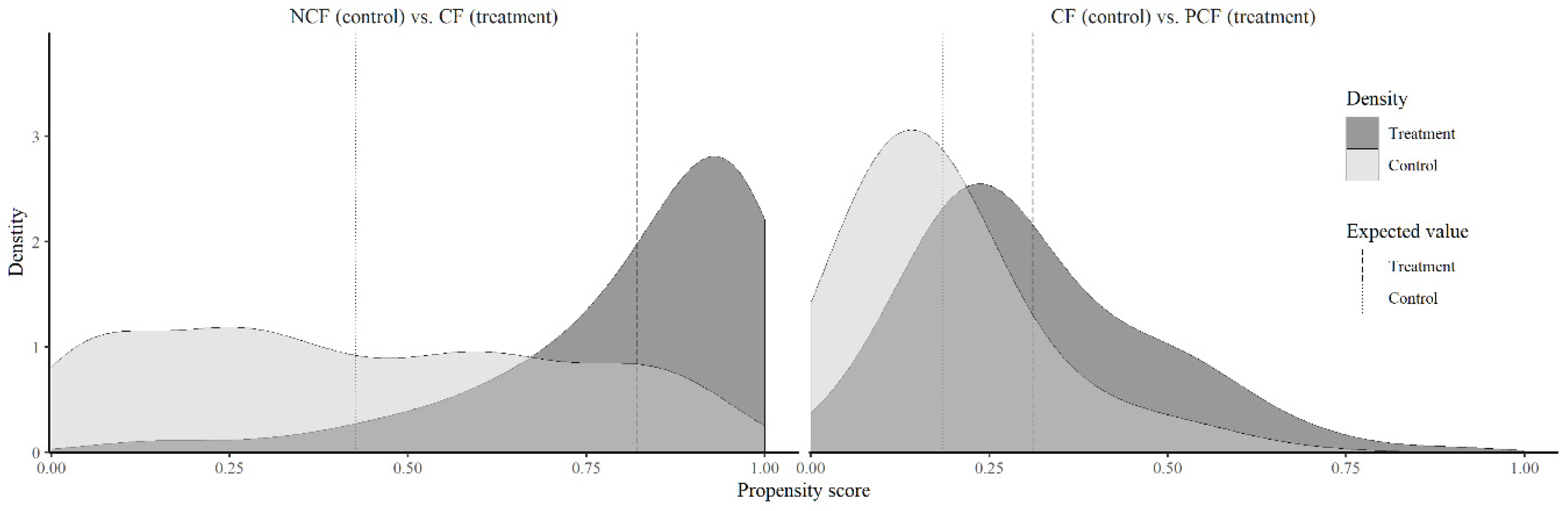
3.1. Propensity Scores (PSs) by Probit Estimations

Table 2. Results of probit estimation.

	NCF vs. CF		CF vs. PCF
	Average Marginal Effect	p-Value	Average Marginal Effect	p-Value
NCOM	0.014 ***	0.000	0.004 *	0.058
FHH	0.156 ***	0.000	−0.050	0.472
FHH2	−0.015 *	0.062	0.003	0.803
PFARM	0.207	0.128	0.435 **	0.037
NFARM	0.000	0.900	0.000	0.637
AAREA	0.038	0.579	0.163 **	0.045
RENTOUT	0.007 **	0.021	0.000	0.987
OV5	−0.002	0.833	−0.028 *	0.061
SUCCESS	−0.014 ***	0.000	0.006	0.192
AGEU40	−0.006	0.120	−0.003	0.552
RICE	0.003 ***	0.000	−0.003 *	0.052
MEET	0.067 *	0.086	0.221 **	0.039
MEET2	−0.003	0.661	−0.071 **	0.024
MPS	0.028	0.535	−0.005	0.940
DPHM	0.101 ***	0.001	−0.067	0.126
DEPOP	0.101 ***	0.007	−0.086 *	0.084
SLOPE	0.000	0.357	0.000	0.708
HMA	0.027	0.412	0.009	0.839
KYOTO	−0.053	0.111	0.171 ***	0.000
SHIGA	0.126 ***	0.009	−0.082	0.164
Regional controls: LR test (χ2)	14.4 ***		21.5 ***
Number of observations	732		514
Log-likelihood	−290.0		−232.7
McFadden’s pseudo R2	0.402		0.140

Note: *, **, and *** indicate statistical significance at the 10%, 5%, and 1% levels, respectively.

shows the probit model results for the CF model, with CF as the treatment, and the PCF model, with PCF as the treatment. First, McFadden’s pseudo R² for the CF model is about 0.406, which is a good fit, whereas the result for the PCF model is merely acceptable (0.140). In addition, PCF models tend to have fewer significant coefficients. This is likely due to the inefficiency of the estimation because the NCF group observations are removed from the sample in the PCF model. Regarding the control by regional dummies, the likelihood ratio (LR) test was significant for both models, indicating that regional differences exist and are well-controlled.

NCOM is positive and significant in both models. As for FHH, an inverse U-shaped relationship was observed in the CF model, which is consistent with the results of Ito et al. [3]. These coefficients indicate that the optimal community size for CF formation is about 52 ($520.156÷0.015÷2\times 10$) farm households. Because the average number of farms in a village is 15.3 (Table 1), it is appropriate to assume that the marginal effect of the number of farms decreases. The proportion of part-time farmers (PFARM) has a positive effect on PCF formation, possibly due to a strong desire to save labor in managing CPRs. AAREA is also positively significant only for PCF formation. If the average cultivated area is large, the transaction cost per unit area when forming the PCF decreases, which is an expected result. RENTOUT, which indicates land liquidity, also has a positive relationship with CF formation, showing that the lower the transaction costs, the easier it is to form the CF.

The presence of large-scale farmers (OV5) is a barrier to the formation of PCFs. For SUCCESS and AGEU40, only the former is negatively significant regarding CFs, indicating that the necessity of forming a CF is reduced when there is a successor for the agricultural management entity. RICE was positively significant, which means that dependence on rice accelerates the need for CF formation in each community. However, the dependence on rice has a negative effect on the formation of PCFs. The reason for this is not clear, but the reciprocity in rice production may be relatively localized and, therefore, may not be compatible with wider PCFs. MEET was considered a proxy variable for social capital in the community, with a positive effect for CFs and an inverted U-shape for PCFs (optimally 15 times per year). Areas with more social capital promote CF formation, consistent with Kitano [39], demonstrating that participants contribute to decision-making in the introduction of environmentally friendly agriculture in communities.

MPS and DPHM are both policy-related variables. MPS has no effect, whereas DPHM has a positive effect on CF formation. Although any group may receive an MPS subsidy, a DPHM subsidy requires an agreement between the community and the municipality. Therefore, it is highly likely that past experiences with the decision-making process have a positive effect on CF formation. Of the three variables (DEPOP, SLOPE, and HMA) indicative of regional disadvantage, only DEPOP has a significant effect. In depopulated areas, the labor shortage has a positive effect on CF formation because it is necessary to form CFs to carry out collective actions toward the conservation of CPRs and farmland. However, for wide-area activities such as PCFs, this has a negative impact, as there are not enough human resources available in such areas. Finally, among the regional dummies, SHIGA for CFs and KYOTO for PCFs are significant, controlling for prefecture-specific characteristics and policies appropriately.

Finally, Figure 4 shows the distribution of estimated propensity scores. These figures compare the kernel density distributions of PSs estimated from the probit models between the treatment and the control groups. To implement PSM, both groups of PSs must overlap (i.e., the common support condition) [41]. In both models, most of the distributions of the PSs overlap, but in some areas, for example, where the probability of the CF model is low or the probability of the PCF model is high, the density of the PSs of both groups is low. Therefore, we set a criterion of 0.05 times the standard deviation (i.e., caliper) during the matching procedure to satisfy the common support condition, which dropped nine and five observations in the CF and PCF models, respectively.

3.2. Average Treatment Effect (ATE)

First, we examine the balancing property (BP) of covariates after matching. Confirmation of the BP is a common procedure to ensure that covariates are balanced between the treatment and control groups after matching, thereby meeting the CIA. In our analysis, we used standard BP measures—the standardized mean difference (SMD) and the variance ratio (VR) [43,54]—which are shown in Appendix A

Table A2. Balancing properties of covariates after PSM.

	NCF vs. CF				CF vs. PCF
	SMD		VR		SMD		VR
	Raw	Matched	Raw	Matched	Raw	Matched	Raw	Matched
NCOM	0.490	0.031	0.355	1.393	0.490	0.031	0.355	1.393
FHH	0.373	0.109	1.321	1.121	0.373	0.109	1.321	1.121
FHH2	0.168	0.085	1.057	0.677	0.168	0.085	1.057	0.677
PFARM	0.314	0.093	2.537	1.162	0.314	0.093	2.537	1.162
NFARM	0.288	0.043	0.584	0.683	0.288	0.043	0.584	0.683
AAREA	0.278	0.057	1.366	0.776	0.278	0.057	1.366	0.776
RENTOUT	0.381	0.010	0.855	1.059	0.381	0.010	0.855	1.059
OV5	0.144	0.073	2.355	0.928	0.144	0.073	2.355	0.928
SUCCESS	0.539	0.084	2.788	0.837	0.539	0.084	2.788	0.837
AGEU40	0.025	0.004	1.327	0.867	0.025	0.004	1.327	0.867
RICE	0.647	0.065	3.833	1.467	0.647	0.065	3.833	1.467
MEET	0.682	0.087	1.046	1.036	0.682	0.087	1.046	1.036
MEET2	0.406	0.047	0.467	0.812	0.406	0.047	0.467	0.812
MPS	0.180	0.117	0.973	0.819	0.180	0.117	0.973	0.819
DPHM	0.682	0.175	1.184	2.403	0.682	0.175	1.184	2.403
DEPOP	0.026	0.156	0.949	0.783	0.026	0.156	0.949	0.783
SLOPE	0.254	0.073	0.888	0.993	0.254	0.073	0.888	0.993
HMA	0.183	0.099	1.043	0.933	0.183	0.099	1.043	0.933
KYOTO	0.325	0.249	1.351	1.143	0.325	0.249	1.351	1.143
SHIGA	0.387	0.059	0.553	0.901	0.387	0.059	0.553	0.901

. The lower the SMD, the smaller the difference between the two groups, and the closer the VR is to 1, the more likely that it is both groups are random variables from the same distribution. In both models, these indices after matching are significantly improved compared to those of the raw data. Therefore, we judge that the CIA requirements were met (randomization was secured).

Table 3. Estimation results of ATEs from PSM.

	CF (vs. NCF)				PCF (vs. CF)
	Control	Treatment	ATE		Control	Treatment	ATE
	Mean	Mean	Estimates	p-Value	Mean	Mean	Estimates	p-Value
CONSERV	47.896	65.530	17.634 ***	0.000	72.173	65.844	−6.328 ***	0.000
ABANDON	6.901	6.330	−0.571 *	0.051	5.931	5.970	0.039	0.902
SALE500	6.158	6.147	−0.011	0.981	5.390	4.670	−0.720 **	0.027

Note: *, **, and *** indicate statistical significance at the 10%, 5%, and 1% levels, respectively.

shows the final ATE estimation results. First, for the CF model, the effect on CONSERV is positive and significant at the 1% level, indicating that CF formation contributes to the conservation of CPRs. ABANDON is also negatively significant; thus, CFs prevent the occurrence of abandoned farmland. However, SALE500 is not significant and the coefficient value is low. Conversely, in the PCF model, the ATE of CONSERV is negatively significant, which means that PCF formation might in some cases have a negative effect on CPR conservation, contrary to the CF model. The PCF formation effect on abandoned farmland (ABANDON) is not significant, but PCF formation has a negative effect on the proportion of large-scale farmers (SALE500). The most surprising result is that the ATEs for CONSERV and SALE500 in the PCF model both show a negative effect, suggesting that the formation of PCFs could, on average, lead to a decline in CPR conservation and a decrease in the number of large farms.

3.3. Robustness Check and Heterogeneous Treatment Effect

We checked the robustness of our estimates from the previous subsection by comparing the results from alternative IPTW methods.

Table 4. Estimation results of ATEs from IPTW method.

	Normal IPTW				Stabilized IPTW
	CF (vs. NCF)		PCF (vs. CF)		CF (vs. NCF)	PCF (vs. CF)
	Coefficient	Std Error	Coefficient	Std Error	Std Error	Std Error
CONSERV	12.561 ***	2.440	−5.138 **	2.447	*** 2.763	* 3.062
ABANDON	−1.761 ***	0.425	−0.526	0.431	*** 0.469	0.544
SALE500	−1.249 **	0.614	−0.249	0.480	* 0.653	0.630

Note: *, **, and *** indicate statistical significance at the 10%, 5%, and 1% levels, respectively. The estimated values using the stabilized ATE weight are the same as those of the normal IPTW, so the coefficients are not shown.

shows the results of the IPTW estimation. The disadvantage of the IPTW estimator is that when the PSs are low, the weight of the inverse probabilities is high; therefore, when there are many such observations, the standard error of the estimated value is high. The PCF model has many observations with low PSs, as shown in Figure 4. Therefore, the efficiency of the estimation may be impaired. The right side of the table also shows the results of the estimation using a stabilized ATE weight designed to reduce the instability of the estimate due to extremely high weights [55]. The signs and effects of the ATEs that are significant in either normal matching or the IPTW estimation are similar, so the ATE estimation result is robust. However, for SALE500, care must be taken because significant results have shifted from PCFs to CFs.

Finally, we examine the heterogeneity of the treatment effect on each outcome of CF and PCF formation using the matching-smoothing method [56]. We regressed each treatment effect on PSs using a nonparametric method: locally weighted scatterplot smoothing (LOESS). Figure 5 plots the estimated smoothing curve, with the gray zone indicating the 95% confidence interval. That is, if there are any two points between which the confidence intervals do not overlap, the treatment effects may differ depending on the PSs (i.e., the state of covariates). Focusing on the case in which the ATEs are significant, heterogeneities can be observed in CONSERVE and ABANDON in CF formation (upper row). Regarding CONSERV, treatment effects are low in the zone with low PSs but are high in the zone with high PSs. Conversely, for ABANDON, treatment effects are high in the zone with low PSs (the effect of preventing abandoned farmland is high) but low in the zone with high PSs.

Various studies have argued that external interventions can either enhance or harm intrinsic motivations [57]. Ito et al. [3] examine the effectiveness of the MPS treatment and observe that it diminishes according to the probability of participation in the MPS program. They argue that, if intrinsic motivations are inherent in the local community based on the belief that the conservation of CPRs should be done voluntarily, extrinsic systems such as subsidies crowd out these motivations. Applying the same logic to our results, the formation of CFs crowds in intrinsic motivations for CPR conservation activities but crowds out motivations for the prevention of abandoned farmland. Generally, in Japan, farmers form CFs to coordinate the agricultural labor force and capital and reduce the burden of collective actions [27], but they also need to manage CFs effectively and economically. Therefore, cultivating more poorly conditioned farmland as a result of widening the area of CFs (PCFs) leads to a larger labor and economic burden. A high motivation to support regional agriculture and the economy through the formation of CFs can result in abandoned farmland.

4. Discussion

Our results prove that CF formation is effective in preserving CPRs and preventing abandoned farmland, as the relevant policies generally expect. In other words, measures to promote the formation of CFs by MAFF have been successfully contributing toward making local agriculture and resource management sustainable. However, these measures could also reduce the proportion of large-scale farmers (Table 4). We cannot immediately infer from our analysis whether this is due to CF formation omitting large-scale farmers or the low production efficiency of formed CFs. This is an empirical task for the future.

The most important implication of this study is that among the average treatment effects of PCFs, the effect on CONSERV is clearly negative. This means that some areas where PCFs are formed tend to neglect CPR conservation activities. If such results are observed or predicted by farmers in other areas, they would hesitate to form a PCF. Given that the proportion of PCF formation in our study area is the lowest in the country, it is reasonable for farmers to avoid the negative effects of forming a CF partnership. From a different perspective, the optimal CF size for CPR conservation is likely to be smaller than the current average PCF size. In fact, in rural areas of Japan, when CFs form a PCF, this organization offers the advantages of efficiency in machine utilization and ease of recruiting human resources [34]. However, the costs of land accumulation, coordinating the production systems between regions, and communication (conflict resolution) are challenges that need to be overcome [33]. Therefore, governments and local agricultural cooperatives (JA) need to make efforts to reduce transaction costs through projects that support the construction of production systems that match local land conditions and the development of leaders (human capital).

PCFs may also have a negative effect on the ratio of large-scale farmers (SALE500) on average (Table 3). Following the same deduction as CONSERVE, the low level of PCF formation in our study area may be a result of the farmers’ economically rational behavior. This may be because wide-area PCF formations have caused many residents to rely on those organizations for CPR conservation activities that were previously performed well at the community level. In addition, the formation of such an organization can crowd out the motivations for conservation activities and thereby reduce their implementation ratio. However, it should be noted that these results may be limited to areas with specific characteristics. Because our study area has abundant part-time job opportunities near metropolitan areas and is highly dependent on rice production, there may be an optimal area size for CFs. As Bowles [58] points out, well-designed policy promotions crowd in the motivations that people originally have but can be counterproductive. Therefore, it is important to provide policy support tailored to local conditions, rather than forcibly promoting the formation of wide-area CFs in such areas.

Our analysis used the latest available data as of 2015. However, CFs have been able to receive additional subsidies as part of the DPHM policy by agreeing on regional partnerships between communities since 2016 [59]. These new policies were likely established because while almost all rural areas in Japan have been underpopulated and aging, widespread cross-community collaboration has not been progressing either. To date, there are still only 173 CFs with agreements and financial support under the new policy (i.e., PCFs) nationwide, which is 0.1% of all communities. Generally, farmers are reluctant to enter into such agreements because of the heavy burden of administrative work and obligatory performance reporting. Disadvantaged areas lack human resources; thus, the government should focus on reducing the administrative work as well as compensating for the agricultural labor cost.

Finally, we discuss some limitations of our analysis. First, the shrinkage and collapse of farmers’ motivations may be a region-specific phenomenon in areas with many paddy fields or near large cities. Therefore, it is unclear whether the same effects of CF and PCF formation are detected in other regions, meaning that the external validity of our results is limited. In the future, an analysis using data from other regions and wider areas will be required. Another problem of our analysis is that farmers’ decision-making regarding CF formation may not be evolutionary and ordinal as we assumed. For example, there may be cases in which a wide-area PCF is formed at the initial decision-making stage. Although we assumed the order of NCF, CF, and PCF, there may be cases in which an NCF evolves directly to the PCF stage. To model such decision-making, it might be better to use a multinomial model. Additionally, CFs were coded based on whether they existed in an FMA but the organization rate is continuous. These effects cannot be taken into account in our analysis. These points will be considered for future research.

5. Conclusions

In this study, we examined drivers and barriers that affect the formation and development of community farms (CFs). More importantly, we analyzed the effects the formation of CFs and PCFs (CFs in partnership with other CFs) on local performance indicators using a causal inference framework. Regarding the CF formation factors, robust results were derived that mostly support our hypotheses. We found that these important factors are farmlandaff transaction costs, the presence of young farmers and successors, and the accumulation of local social capital.

More importantly, there was a clear difference between the treatment effects of CFs and PCFs. Positive effects of CF formation on CPR conservation and prevention of abandoned farmland were detected. However, PCF formation had negative average treatment effects on CPR conservation, which supports our most important hypothesis that CF spatial evolution (PCF) can impair the conservation of CPRs. Moreover, our results indicate that the formation of a wide-area agricultural organization could crowd out local people’s motivations for collective actions and consequently impede existing CPR conservation activities. Therefore, when implementing policies related to community farms, it is more important to take into account an optimal scale of local organization and regional conditions and to reduce transaction costs and administrative work, rather than to forcibly develop and expand community farms through policy measures.

References

1. Wade, R. The Management of Common Property Resources: Finding a Cooperative Solution. World Bank Res. Obs. 1987, 2, 219–234. [Google Scholar] [CrossRef] [Green Version]
2. FAO. Governing Tenure Rights to Commons. Available online: http://www.fao.org/family-farming/detail/en/c/1027659/ (accessed on 25 March 2020).
3. Ito, J.; Feuer, H.N.; Kitano, S.; Komiyama, M. A Policy Evaluation of the Direct Payment Scheme for Collective Stewardship of Common Property Resources in Japan. Ecol. Econ. 2018, 152, 141–151. [Google Scholar] [CrossRef]
4. Ostrom, E.; Gardner, R. Coping with Asymmetries in the Commons: Self-Governing Irrigation Systems Can Work. J. Econ. Perspect. 1993, 7, 93–112. [Google Scholar] [CrossRef]
5. Shogenji, S. Japan’s Position in the Context of Agricultural Trade Issues. Jpn. J. Agric. Econ. 2019, 21, 56–62. [Google Scholar] [CrossRef]
6. Tada, R.; Ito, J. The Economic Performance of Paddy Field Farming in Japan and the Causal Effect of Direct Payments. J. Rural Econ. 2018, 89, 261–276. [Google Scholar] [CrossRef]
7. Ito, J.; Feuer, H.N.; Kitano, S.; Asahi, H. Assessing the effectiveness of Japan’s community-based direct payment scheme for hilly and mountainous areas. Ecol. Econ. 2019, 160, 62–75. [Google Scholar] [CrossRef]
8. MAFF. Summary of the Basic Plan for Food, Agriculture and Rural Areas—Food, Agriculture and Rural Areas Over the Next 10 Years. Available online: https://www.maff.go.jp/e/policies/law_plan/index.html (accessed on 15 March 2020).
9. Chen, S.; Lan, X. There Will Be Killing: Collectivization and Death of Draft Animals. Appl. Econ. 2017, 9, 58–77. [Google Scholar] [CrossRef] [Green Version]
10. Brooks, K.; Lerman, Z. Land Reform and Farm Restructuring in Russia: 1992 Status. Am. J. Agric. Econ. 1993, 75, 1254–1259. [Google Scholar] [CrossRef] [Green Version]
11. Ravenscroft, N.; Moore, N.; Welch, E.; Hanney, R. Beyond Agriculture: The Counter-Hegemony of Community Farming. Agric. Hum. Values 2013, 30, 629–639. [Google Scholar] [CrossRef] [Green Version]
12. Liu, P.; Gilchrist, P.; Taylor, B.; Ravenscroft, N. The Spaces and Times of Community Farming. Agric. Hum. Values 2017, 34, 363–375. [Google Scholar] [CrossRef] [Green Version]
13. Matsuno, Y.; Nakamura, K.; Masumoto, T.; Matsui, H.; Kato, T.; Sato, Y. Prospects for Multifunctionality of Paddy Rice Cultivation in Japan and Other Countries in Monsoon Asia. Paddy Water Environ. 2006, 4, 189–197. [Google Scholar] [CrossRef]
14. Sato, H. Toward Preservation of the Multi-Functional Roles of Paddy Field Irrigation. Paddy Water Environ. 2005, 3, 1–3. [Google Scholar] [CrossRef]
15. Fujiie, M.; Hayami, Y.; Kikuchi, M. The Conditions of Collective Action for Local Commons Management: The Case of Irrigation in the Philippines. Agric. Econ. 2005, 33, 179–189. [Google Scholar] [CrossRef]
16. Narloch, U.; Pascual, U.; Drucker, A.G. Collective Action Dynamics Under External Rewards: Experimental Insights from Andean Farming Communities. World Dev. 2012, 40, 2096–2107. [Google Scholar] [CrossRef]
17. Takeda, M.; Takahashi, D.; Shobayashi, M. Collective Action vs. Conservation Auction: Lessons from a Social Experiment of a Collective Auction of Water Conservation Contracts in Japan. Land Use Policy 2015, 46, 189–200. [Google Scholar] [CrossRef]
18. MAFF. FY2017: Summary of the Annual Report on Food, Agriculture and Rural Areas in Japan. Available online: https://www.maff.go.jp/e/data/publish/index.html#Annual (accessed on 25 March 2020).
19. Andou, M. Possibilities and Limitations of Restructuring Paddy Field Farming by Group Farming Based on Community-Focusing on the Regional Diversity Reflecting Its Agricultural Structure. J. Rural Econ. 2008, 80, 67–77. [Google Scholar] [CrossRef]
20. Feldhoff, T. Shrinking Communities in Japan: Community Ownership of Assets as a Development Potential for Rural Japan? Urban Des. Int. 2013, 18, 99–109. [Google Scholar] [CrossRef] [Green Version]
21. Ostrom, E. Analyzing Collective Action. Agric. Econ. 2010, 41, 155–166. [Google Scholar] [CrossRef]
22. Olson, M. The Logic of Collective Action: Public Goods and the Theory of Groups; Harvard University Press: Cambridge, MA, USA, 2009. [Google Scholar]
23. Poteete, A.R.; Ostrom, E. Heterogeneity, Group Size and Collective Action: The Role of Institutions in Forest Management. Dev. Chang. 2004, 35, 435–461. [Google Scholar] [CrossRef]
24. Agrawal, A. Small Is Beautiful, but Is Larger Better? Forest-Management Institutions in the Kumaon Himalaya, India. In People and Forests: Communities, Institutions, and Governance; MIT Press: Cambridge, MA, USA, 2000; pp. 57–86. [Google Scholar]
25. Baland, J.-M.; Platteau, J.-P. Co-Management as a New Approach to Regulation of Common Property Resources. In Halting Degradation of Natural Resources; Baland, J.-M., Platteau, J.-P., Eds.; Oxford Scholarship Online: Oxford, UK, 2005. [Google Scholar] [CrossRef]
26. Rosenbaum, P.R.; Rubin, D.B. The Central Role of the Propensity Score in Observational Studies for Causal Effects. Biometrika 1983, 70, 41–55. [Google Scholar] [CrossRef]
27. Katsura, A. Perspective of Agricultural Structure Reform and Village-based Group Farming. J. Rural Probl. 2005, 40, 381–392. [Google Scholar] [CrossRef] [Green Version]
28. Hiratsuka, T. On the Group Farming Based on the Village as a Farm Management: Its Definition, Significances, and Tasks of Formation and Development. J. Rural Probl. 1992, 28, 80–90. [Google Scholar] [CrossRef] [Green Version]
29. Tashiro, Y. Incorporation by Community Farming and Individual Farmers: Ooasa-cho, Higashihiroshima City, Hiroshima Prefecture. In Formation of Agricultural Organization in Japan; Tashiro, Y., Ed.; Tsukuba Shobo: Tokyo, Japan, 2006; ISBN 978-4-8119-0309-5. [Google Scholar]
30. Ito, J.; Nishikori, M.; Toyoshi, M.; Feuer, H.N. The Contribution of Land Exchange Institutions and Markets in Countering Farmland Abandonment in Japan. Land Use Policy 2016, 57, 582–593. [Google Scholar] [CrossRef]
31. MAFF. Notice: About Promotion of Future Agricultural Leader Policy. Available online: https://www.maff.go.jp/j/kokuji_tuti/tuti/t0000741.html (accessed on 10 March 2020).
32. Miyatake, K. Development of Combined Community-based Group Farms. Jpn. J. Farm Manag. 2007, 45, 41–45. [Google Scholar] [CrossRef]
33. Tanada, M. A Study of Regional Support System by Large Area Cooperation of Village-based Group Farming. Jpn. J. Farm. Manag. 2010, 48, 73–77. [Google Scholar] [CrossRef]
34. Egawa, A. Current Status of Community Activities and Their Movement Toward Wide Area. Available online: https://www.maff.go.jp/primaff/kanko/project/27saisei1.html (accessed on 20 January 2020).
35. Ohnaka, K.; Andou, M. Conditions for and Prospects of Large Scale Community-based Farms: A Case Study of Hakusan City, Ishikawa Prefecture. J. Rural Econ. 2015, 87, 150–155. [Google Scholar] [CrossRef]
36. MAFF. Report: 2020 Survey on Community-Based Cooperatives. 2020. Available online: https://www.maff.go.jp/j/tokei/kouhyou/einou/ (accessed on 2 June 2020).
37. MAFF. Survey on Community-Based Farm Cooperatives. Available online: https://www.maff.go.jp/j/tokei/census/shuraku_data/2015/se/index.html (accessed on 2 January 2020).
38. Kinki Regional Agricultural Administration Office. Overview of Agriculture in Kinki District. Available online: https://www.maff.go.jp/kinki/toukei/toukeikikaku/gaiyo/kinkigaiyo/saisin.html (accessed on 18 March 2020).
39. MAFF. 2015 Census of Agriculture and Forestry in Japan Report and Data on the Result. Available online: https://www.maff.go.jp/e/data/stat/index.html (accessed on 10 January 2020).
40. MAFF. Agricultural Production Income Statistics. Available online: https://www.maff.go.jp/j/tokei/kouhyou/nougyou_sansyutu/ (accessed on 22 February 2020).
41. Guo, S.; Fraser, M.W. Propensity Score Analysis: Statistical Methods and Applications; Sage: Thousand Oaks, CA, USA, 2015; ISBN 978-1-4522-3500-4. [Google Scholar]
42. Holland, P.W. Statistics and Causal Inference. J. Am. Stat. Assoc. 1986, 81, 945–960. [Google Scholar] [CrossRef]
43. Stuart, E.A. Matching Methods for Causal Inference: A Review and a Look Forward. Stat. Sci. 2010, 25, 1–21. [Google Scholar] [CrossRef] [Green Version]
44. Rosenbaum, P.R.; Rubin, D.B. The Bias Due to Incomplete Matching. Biometrics 1985, 41, 103–116. [Google Scholar] [CrossRef]
45. Sekhon, J.S. Multivariate and Propensity Score Matching Software with Automated Balance Optimization: The Matching Package for R. J. Stat. Softw. 2011, 42, 52. [Google Scholar] [CrossRef] [Green Version]
46. MAFF. Comprehensive Database Based Mainly on Agricultural and Forestry Census. Available online: https://www.maff.go.jp/j/tokei/census/shuraku_data/ (accessed on 10 March 2019).
47. Ministry of Health, Labour and Welfare of Japan. Annual Health, Labour and Welfare Report 2017. Available online: https://www.mhlw.go.jp/english/wp/w0p-hw11/index.html (accessed on 4 June 2020).
48. Kitano, S. An Evaluation of a Direct Payment Policy for Community-based Environmental Conservation Agricultural Practices: A Case of Shiga Prefecture in Japan. J. Environ. Inf. Sci. 2019, 2019, 43–52. [Google Scholar] [CrossRef]
49. Yang, W.; Liu, W.; Viña, A.; Tuanmu, M.-N.; He, G.; Dietz, T.; Liu, J. Nonlinear Effects of Group Size on Collective Action and Resource Outcomes. Proc. Natl. Acad. Sci. USA 2013, 110, 10916. [Google Scholar] [CrossRef] [Green Version]
50. Bowles, S.; Gintis, H. Social Capital and Community Governance. Econ. J. 2002, 112, F419–F436. [Google Scholar] [CrossRef]
51. Furuzawa, S.; Kiminami, L. Study on Collective Management of Rural Common-pool Resources and Social Capital. J. Rural Plan. Assoc. 2009, 28, 121–127. [Google Scholar] [CrossRef]
52. Yamaguchi, S.; Nakatsuka, M.; Hoshino, S. Study on Region Characteristic and Settlement in Rural Area—A case of Sasayama city, Hyogo Prefecture. J. Rural Plan. Assoc. 2007, 26, 287–292. [Google Scholar] [CrossRef] [Green Version]
53. Ishihara, H.; Pascual, U. Social Capital in Community-Level Environmental Governance: A Critique. Ecol. Econ. 2009, 68, 1549–1562. [Google Scholar] [CrossRef]
54. Zhang, Z.; Kim, H.J.; Lonjon, G.; Zhu, Y. Balance Diagnostics After Propensity Score Matching. Annu. Transl. Med. 2019, 7, 16. [Google Scholar] [CrossRef]
55. Xu, S.; Ross, C.; Raebel, M.A.; Shetterly, S.; Blanchette, C.; Smith, D. Use of Stabilized Inverse Propensity Scores as Weights to Directly Estimate Relative Risk and Its Confidence Intervals. Value Health 2010, 13, 273–277. [Google Scholar] [CrossRef] [Green Version]
56. Xie, Y.; Brand, J.E.; Jann, B. Estimating Heterogeneous Treatment Effects with Observational Data. Sociol. Methodol. 2012, 42, 314–347. [Google Scholar] [CrossRef]
57. Rode, J.; Gómez-Baggethun, E.; Krause, T. Motivation Crowding by Economic Incentives in Conservation Policy: A Review of the Empirical Evidence. Ecol. Econ. 2015, 117, 270–282. [Google Scholar] [CrossRef]
58. Bowles, S. Policies Designed for Self-Interested Citizens May Undermine “The Moral Sentiments”: Evidence from Economic Experiments. Science 2008, 320, 1605. [Google Scholar] [CrossRef] [PubMed] [Green Version]
59. MAFF. About Direct Payment to Farmers in Hilly and Mountainous Areas. Available online: https://www.maff.go.jp/j/nousin/tyusan/siharai_seido/s_about/index.html (accessed on 3 March 2020).
Figure 1. Conditions of community farms and conservation activities in former municipal level areas (FMAs) in the study area. Source: Survey on Community-based Farm Cooperatives and agricultural census surveys by Japan’s Ministry of Agriculture, Forestry and Fisheries (MAFF).
Sustainability 12 05137 g001
Figure 2. Percentage of communities with community farms (CFs) and multi-CF partnership organizations (PCFs). Source: Survey on Community-based Farm Cooperatives by MAFF.
Sustainability 12 05137 g002
Figure 3. Distributions of outcomes. Note: Each notch and cross mark represent the 95% confidence interval of the median and mean value, respectively. Source: Survey on Community-based Farm Cooperatives and agricultural census surveys by MAFF.
Sustainability 12 05137 g003
Figure 4. Distribution of propensity scores between treatment and control groups.
Sustainability 12 05137 g004
Figure 5. Heterogeneity of treatment effects.
Sustainability 12 05137 g005